Article

Research on Rigid–Elastic Coupling Flight Dynamics of Hybrid Wing Body Based on a Multidiscipline Co-Simulation

School of Aeronautic Science and Engineering, Beihang University, Beijing 100191, China
*
Author to whom correspondence should be addressed.
Appl. Sci. 2023, 13(1), 410; https://doi.org/10.3390/app13010410
Submission received: 11 December 2022 / Revised: 21 December 2022 / Accepted: 25 December 2022 / Published: 28 December 2022
(This article belongs to the Topic Computational Fluid Dynamics (CFD) and Its Applications)

Abstract

:
Due to the special aerodynamic layout and mass distribution, the natural frequency differences between the hybrid wing body (HWB)’s rigid-body motion modes and the fuselage structure elastic modes are smaller compared to conventional aircraft, resulting in the disappearance of the decoupling relationship between the HWB’s rigid-body motion and the elastic motion of the airframe structure. For the above reason, the traditional analysis approach based on the rigid-body assumption is no longer applicable when analyzing the flight dynamics of an HWB aircraft, and a shift must be made to an analysis method that takes into account aeroelastic effects. Therefore, in this paper, a time-domain co-simulation program combining the computational fluid dynamics (CFD) method with computational structure dynamics (CSD) and rigid-body dynamics (RBD) is developed to investigate the effect of a rigid–elastic coupling effect on the flight dynamics of the HWB and this co-simulation method is more advantageous in the calculation of unsteady aerodynamics compared to existing methods of rigid–elastic coupling dynamics analysis. By means of the co-simulation technology, this paper completed a series of simulations, based on which the influence of rigid–elastic coupling effect on the short-period dynamic characteristics of aircraft was studied.

1. Introduction

With the rapid development of aviation technology, modern aircraft such as long-endurance unmanned aircraft, large transport aircraft and large civil airliners are characterized by light weight, low damping and large flexibility due to the high flight performance requirements [1,2,3,4,5,6]. As a result, aeroelasticity has become an important factor that cannot be ignored in the design of these aircraft; rigid–elastic dynamics coupling is one of the aeroelasticity problems of aircraft, and this problem is pronounced in HWB civil airliners due to their unique structural layout and mass distribution. On the one hand, the structure of HWB aircraft is quite flexible, which leads to a low natural frequency of the first-order elastic mode of HWB. For example, Boeing’s preliminary high-speed civil transport has a first-order symmetric bending mode with a natural frequency of 1.4 Hz [7]; on the other hand, the HWB aircraft has a relatively small rotational inertia about the pitch axis, resulting in a higher short-period mode frequency [8,9,10,11]. The above two facts cause the difference between the frequencies of the rigid body motion mode and the aircraft structure elastic mode of the HWB to become smaller, which eventually leads to the coupling problem between the rigid body motion and the structural elastic motion of the HWB configuration to be more obvious than that of the conventional configuration. The decoupling relationship between the rigid body motion and the elastic structure motion of HWB aircraft is no longer obvious or even non-existent. For the above reason, the traditional analysis approach based on the rigid-body assumption is no longer applicable when analyzing the flight dynamics of an HWB aircraft, and a new analysis method considering aeroelastic factors must be developed. To this end, a series of studies on the rigid–elastic coupling flight dynamics for flexible aircraft have been conducted in the past years [12,13,14,15].
The computation of the unsteady aerodynamic force caused by the rigid-body motion of the aircraft superimposed on the elastic deformation motion of the aircraft structure is an essential part of the rigid–elastic flight dynamics, and the main work of this paper is to establish a rigid–elastic coupling flight dynamics analysis platform from the perspective of using new unsteady aerodynamic force computational method. For the convenience of studying the dynamics and control problems, the double-let method is currently used in studies related to the analysis of rigid–elastic coupling flight dynamics. The state space form of unsteady aerodynamic force by DLM is conducive to being integrated into linear dynamics equations, which is convenient for dynamics analysis and related aeroelastic servo system design [16,17,18,19,20,21]. However, the DLM has the following two deficiencies. Firstly, DLM is more suitable for unsteady aerodynamic calculation in critical states such as flutter motion, while the accuracy of unsteady aerodynamic force in the non-critical state cannot be guaranteed. Secondly, due to the limitation of theoretical assumptions, the computational accuracy of aerodynamic components (such as drag components) on some rigid body degrees of freedom is poor. In order to avoid the two deficiencies of DLM, the CFD method is considered in this paper to compute the unsteady aerodynamic force. The CFD method is directly based on the basic equation of the flow, and with fewer additional assumptions, it can more accurately describe the unsteady aerodynamic force caused by the rigid–elastic coupling motion. However, the unsteady aerodynamic forces obtained by the CFD method are in time-domain form, which cannot be converted into a state-space form such as DLM to facilitate the study of rigid–elastic coupling dynamics. For this reason, this paper plans to rely directly on the time domain analysis to achieve the research on rigid–elastic coupling flight dynamics, and a multidisciplinary co-simulation program including a CFD module is thus needed. In the co-simulation program, the structural dynamics equation, aircraft dynamics equation and fluid equation are solved in a loosely coupled way in the time domain to obtain the data set of time-varying flight parameters. By comparing the flight parameters of the rigid–elastic coupled flight co-simulation with those of the rigid-body flight simulation, the influence of the elastic effect on the flight dynamics could be obtained.
The multidisciplinary co-simulation in this paper is essentially a combination of two technologies—the CFD/CSD coupling computation technology and the numerical virtual flight simulation technology based on CFD/RBD coupling computation [22,23,24,25,26,27]. The CFD/CSD coupling calculation technology has been applicated in various aeroelastic mechanism research and engineering calculations. For example, the geometric nonlinear aeroelastic problems caused by large structural deformation were studied by CFD/CSD coupling technology with the updated Lagrange method [28]. As for the numerical virtual flight simulation technology based on CFD/RBD coupling, it is mainly used to simulate the dynamic process of aircraft in a specific period of time and to study various flight dynamics and control problems based on the simulation data. For example, by solving the unsteady Rans equation, rigid body dynamics equation and control law equation simultaneously, the simulation of the quasi-Cobra maneuver process of third-generation fighter aircraft was realized, and based on a similar simulation, the design of the control law of a missile was accomplished [29,30].
This paper considers constructing the co-simulation of CFD/CSD/RBD by the combination of CFD/CSD coupling calculation technology and CFD/RBD coupling-based numerical virtual flight simulation technology and studying the impact of rigid–elastic coupling effect on aircraft dynamics through this multidisciplinary co-simulation. The whole paper could be divided into the following parts: the overall framework of co-simulation, the development and verification of CFD/CSD coupling solver; the development and verification of CFD/RBD simulator; and the results of multidisciplinary time domain co-simulation and the corresponding discussion.

2. Framework of Co-Simulation

The CSD/CFD co-simulation in this paper includes two computational fields: fluid computational field and solid computational field, and a partition computation mode was adopted to couple the computations of the two fields. Under this mode, the fluid computing field and the structural computing field are solved independently, which makes the calculation program modular and simplifies the modeling process. The classical serial coupling iterative process is used to couple the calculation of the solid field as well as the fluid field. As for the time step approach, this paper adopts the loose coupling method; that is, only one staggered iteration is performed between each time step. Although this method loses some time accuracy, it can ensure low consumption of computing resources and is also the mainstream method of multidisciplinary coupled computing.
As shown in Figure 1, the whole co-simulation program includes three parts: the flight dynamics (RBD) module, the structural dynamics (CSD) module and the fluid dynamics (CFD) module. According to the aerodynamics solution of the t time step by the CFD module, the coordinates of the center of mass and the attitude angles of the aircraft in the t + 1 time step are calculated by the RBD module. The elastic displacement of the aircraft structure under the body reference frame in the t + 1 time step is calculated by the CSD module according to the external forces on the aircraft structure (including the aerodynamic force calculated by the CFD module and the inertial force obtained by the RBD module). After the calculations of the two modules above, the position and Euler angles of the aircraft body, the elastic displacement of the structure and the position of the deflection angle of the control surface (determined by the given control command) on the t + 1 time-step are summarized and processed by the UDF program. The CFD solver then updates the computational mesh based on the position information above and solves the RANS equations based on the new mesh. The resulting aerodynamic forces and moments can then be used in the next round of simulation at time step t + 1.

3. Development and Validation of CFD/CSD Coupled Solvers

The coupling solver consists of the following parts: simulation initialization, aerodynamic calculation, load passing between fluid/solid interface, structural dynamics solving, displacement passing between fluid/solid interface and aerodynamic mesh update.

3.1. Initialization of Simulation

The coupling interface interpolation matrix and structure modal shape matrix are pre-stored into the CFD solver to initialize the simulation. The above matrices must be used in the simulation of each time step and storing the data of matrices in the memory before the simulation can avoid the time consumption of repeated reading of these matrices in every time step.

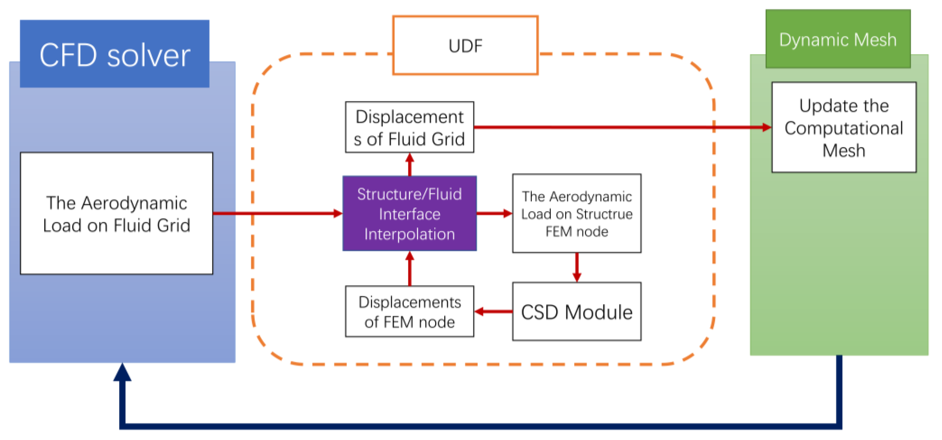
3.2. Structure/Fluid Interface Interpolation

The fluid–solid interface load/displacement transfer is a bidirectional information transfer on the interface between the fluid computing domain and the solid computing domain. Due to the difference in topological form and distribution density between the nodes of fluid mesh and the structural FEM node, the aerodynamic load calculated by CFD on the fluid nodes needs to be transformed into the aerodynamic load on the FEM nodes of the structural model in a solid domain to calculate the structural dynamics through the transfer matrix in the coupling calculation process; on the other hand, the displacement of the FEM nodes obtained by the structural dynamics solver should be transformed into the displacements of the fluid nodes at this time step through the transfer matrix, so as to update the fluid motion boundary required by CFD calculation.
From a mathematical point of view, displacement and load transfer at a fluid/solid interface is an interpolation problem. In this paper, global radial basis functions and monomial basis functions are selected to construct interpolation functions. The radial basis function takes the distance from the target point y to the node x i as its independent variable. As a classical global radial basis function, thin plate spline is widely used in function fitting, and its expression is:
ϕ i ( y ) = d i 2 l n d i , ( i = 1 , 2 , , n s ) ,
where n s is the number of nodes in the domain of definition.
The introduction of the monomial basis function can improve the interpolation accuracy and computational stability. The linear monomial basis of three-dimensional space is:
p ( y ) T = [ 1   x   y   z ] ,   m = 4
where m is the number of elements in the monomial basis function.
The interpolation function u h ( y ) is expressed by thin-plate spline and monomial basis as:
u h ( y ) = i = 1 N a i φ i ( y ) + j = 1 m b j p j ( y ) = Φ T ( y ) a + p T ( y ) b
where N is the number of structural nodes in the domain, a i and b j are undetermined coefficients, φ i are thin plate splines function and p j is a monomial basis function. The corresponding array is defined as:
Φ ( y ) = [ ϕ 1 ( y ) , ϕ 2 ( y ) , , ϕ N ( y ) ] T , p ( y ) = [ p 1 ( y ) , p 2 ( y ) , , p m ( y ) ] T , a = [ a 1 , a 2 , , a N ] T , b = [ b 1 , b 2 , , b N ] T ,  
The interpolation function is forced through the structure nodes in its definition of the domain by Equation (5)
i = 1 N a i φ i ( y ) + j = 1 m b j p j ( y ) = u k , k = 1 , 2 , , N ,  
In order to ensure the uniqueness of monomial base interpolation, additional constraints are imposed:
i = 1 N a i φ i ( y ) = 0 , j = 1 , 2 , , m ,
Written in matrix form:
B [ a b ] = [ u 0 ] ,
where:
B = [ A P P T 0 ] A = [ Φ T ( x 1 ) Φ T ( x 2 ) Φ T ( x N ) ]   = [ ϕ 1 ( x 1 ) ϕ 1 ( x 1 ) ϕ 1 ( x 1 ) ϕ 1 ( x 2 ) ϕ 1 ( x 2 ) ϕ 1 ( x 2 )                                                                   ϕ 1 ( x 2 ) ϕ 1 ( x 2 ) ϕ 1 ( x 2 ) ] P = [ P T ( x 1 ) P T ( x 2 ) P T ( x N ) ]   = [ P 1 ( x 1 ) P 2 ( x 1 ) P m ( x 1 ) P 1 ( x 2 ) P 2 ( x 2 ) P m ( x 2 )                                                                   P 1 ( x 2 ) P 2 ( x 2 ) P m ( x N ) ]
Because ϕ i ( x j ) = ϕ j ( x i ) , is a symmetric matrix. The matrix a and b can be solved from Equation (7) and substituted into Equation (3), thus:
u n ( y ) = [ Φ T ( y ) P T ( y ) ] B 1 [ u 0 ] = [ Φ T ( y ) P T ( y ) ] B 0 u = N ( y ) u ,
where B 0 is the submatrix composed of the first N-column elements of the B 1 matrix. The form function N ( y ) is:
N ( y ) = [ Φ T ( y ) P T ( y ) ] B 0 ,
Accordingly, the interpolation matrix H can be expressed as:
H = [ N ( y 1 ) T N ( y 2 ) T N ( y n f ) T ] T ,
where y i is the coordinates of fluid nodes, and n f is the number of fluid nodes.

3.3. Structural Dynamics Equation

The fluid-structure coupling vibration satisfies the following equation:
M u ¨ + C u ˙ + K u = f ( t ) ,
In the above equation, M , C , K are the mass matrix, damping matrix and stiffness matrix of the system, respectively. u ¨ , u ˙ , u , respectively, correspond to the acceleration, velocity and displacement vector of structure movement; f ( t ) is the time-dependent external excitation on the system. For aeroelastic systems, f ( t ) is the aerodynamic force acting on the structure.
In this paper, the modal coordinate transformation method is used to solve the structural dynamics equation. Introduce coordinate transformation:
u = Φ q ,
In the above equation, u is the coordinate in physical space, and q is the modal coordinate, so:
u ˙ = Φ q ˙         u ¨ = Φ q ¨ ,
Equation (13) and Equation (14) are substituted into Equation (12):
M Φ q ¨ + C Φ q ˙ + K Φ q = f ( t ) ,
Multiply the left and right sides of the equation by Φ T to obtain:
Φ T M Φ q ¨ + Φ T C Φ q ˙ + Φ T K Φ q = Φ T f ( t ) ,
Substituting Equation (14) into Equation (16) yields the following equation.
d i a g [ M r ] q ¨ + Φ T C Φ q ˙ + d i a g [ K r ] q = Φ T f ( t ) ,
In this paper, the damping of the structure is assumed to be 0, and then the above equation can be simplified as follows:
d i a g [ M r ] q ¨ + d i a g [ K r ] q = Φ T f ( t )
For Equation (18), introduce the state variable:
E = [ q q ˙ ]
Combined, Equation (18) can be converted to:
E ˙ = [ 0 I d i a g [ M r ] q ¨ d i a g [ K r ] q 0 ] E + [ 0 d i a g 1 [ M r ] Φ T f ( t ) ]
The classical four-step Runge–Kutta iterative method is adopted to solve the equations, and the iteration format is as follows:
E ( 0 ) = E ( n ) E ( 1 ) = E ( 0 ) + Δ t 2 E ˙ ( 0 )

3.4. Procedure of CFD/CSD Simulation

The computational procedure of CFD/CSD simulation is shown in Figure 2. By taking the simulation of t time-step as an example, the aerodynamic load distribution on each fluid node on the elastic surface, corresponding to the dynamic boundary in the CFD fluid calculation domain, is obtained by the CFD solver first, and the load distribution is the input of the fluid/solid interpolation in the user-defined program. Through the fluid/solid load interpolation, the aerodynamic load distribution on the fluid node can be transformed to be the aerodynamic load on the FEM node of the structure model. With the state variables of each FEM node on the t time step and the aerodynamic load distribution on the structural node just obtained as the input of the CSD calculation module, the position and velocity of each structural FEM node in the t + 1 time step can be obtained.
The displacements of the structural nodes are the input of the fluid/solid interpolation calculation, through which the displacements of each fluid node are obtained. Finally, according to the displacement of these aerodynamic fluid nodes, the fluid computational mesh on the t + 1 time step is updated, and the aerodynamic calculation and simulation of the next time step are carried out.

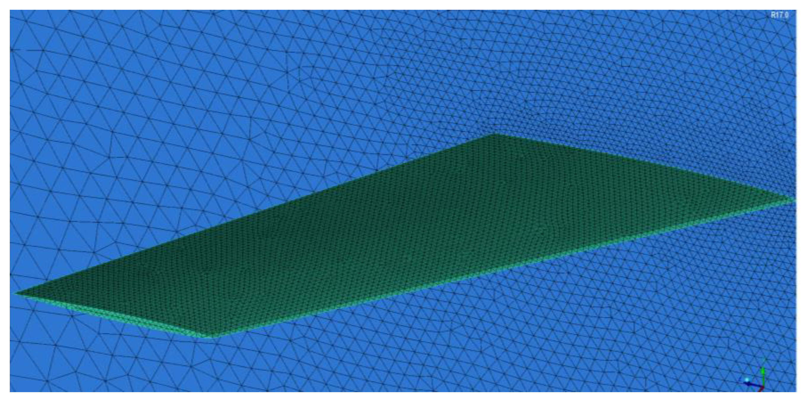
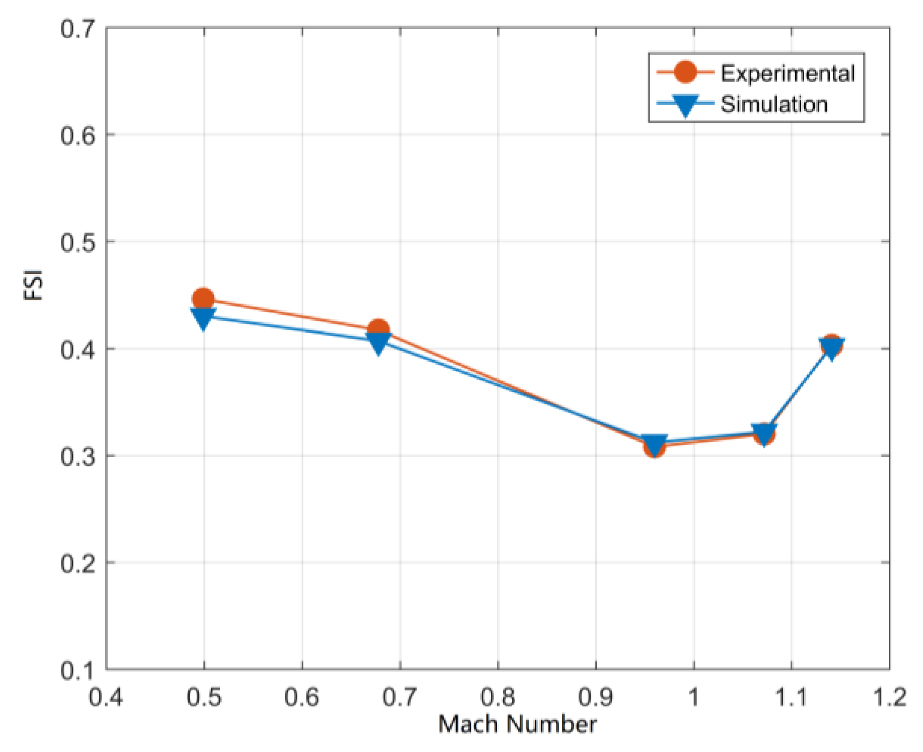
3.5. Verification of the CFD/CSD Co-Simulation

In order to verify the accuracy of transonic unsteady aerodynamic solutions and facilitate their application in the study of aeroelasticity problems, a series of flutter experiments were conducted around the AGARD 445.6 wing in the transonic wind tunnel at NASA Langley Center. In this paper, flutter simulation was carried out for AGARD445.6 wings, and the validity of the CFD/CSD coupling simulation method was verified by comparing the simulation results with the flutter test data of AGARD445.6 wing.
The main attributes of AGARD 445.6 are as follows: the mass of the model is 1.8628 kg, the aspect ratio is 1.6525, the root–tip ratio is 0.6576, the sweep Angle of the 1/4 string is 45°, the airfoil of each station along wingspan is NACA 65A004, and the experimental angle of attack (AOA) is set to zero.
Firstly, according to the geometric size in Figure 3 and the airfoil information of NACA 65A004, the geometric model of AGARD445.6 was established in the 3D modeling software, which served as the basis for the subsequent structural modeling and aerodynamic modeling. Then, in order to obtain the necessary structural modal information for CFD/CSD coupling simulation calculation, the STP format wing model was imported into the finite element software MSC.PATRAN and the structure model of AGARD445.6 wing were established for modal calculation, as shown in Figure 4 below.
Based on the assumption of homogenization, the constructed structural model adopts three-dimensional Hex8-type grid elements, with 3080 elements and 4845 structural nodes. The material directions of the elements are divided into longitudinal and lateral directions, corresponding to the x and y axes of the local coordinate system in the figure, respectively. The material properties of the model are as Table 1:
By transferring the above structural model to MSC.NASTRAN solver, the first several modal information of the wing structural model can be obtained, including natural frequency, mode shape, etc. According to relevant studies, the difference between the flutter velocity calculated by the first four modes and the fourteen modes is less than 1%. Therefore, in the aeroelastic analysis of AGARD445.6, only the first four-order natural modes of the structure should be retained for the subsequent modal superposition method to solve the dynamic response of the structure.
In this paper, the results of the first four-order modal natural frequencies of the AGARD445.6 wing calculated by MSC.NASTRAN were compared with the measured experimental values, as shown in the table below. It can be seen that the calculated values have a good agreement with the experimental values, indicating that the constructed structural model can effectively reflect the structural dynamic characteristics of the real wing.
In addition, the mode shapes of the first four modes were obtained by MSC.NASTRAN are 1 order bending, 2 order torsion, 3 order bending and 4 order torsion, respectively. The experimental values of natural frequencies of the first four modes are compared with the calculated values in this paper, as shown in Table 2.
The aerodynamic model of AGARD445.6 was established in ICEM. The flow field mesh and the wing surface grid is shown in Figure 5. The size of the flow field calculation domain is 14 × 10 × 6 m, and there are six surfaces forming the outer boundary of the flow field. The boundary condition of the side face connected with the wing is set as the wall surface, and the remaining five surfaces are set as the far field.
The nodes of the structural finite element model include external surface nodes and internal structural nodes. The information exchange of aerodynamic force and displacement is realized between the FEM nodes on the outer surface and the aerodynamic grid through interpolation, while the internal nodes of the structure do not participate in the above exchange. However, since both outer surface nodes and inner structural nodes participate in the solution of structural dynamics, the two types of nodes need to be distinguished in the solution process of co-simulation: only outer surface nodes among structural nodes are extracted and used in the CSD/CFD interface interpolation calculation, while all structural nodes are used in the solution of structural dynamics.
The comparison between the flutter boundary predicted by the CFD/CSD program developed in this paper and the experimental results at each Mach number is shown in Figure 6. It can be seen that the difference between the simulation results and the experimental results is small, which proves the validity of the CFD/CSD calculation in this paper. Figure 7 shows two states of whether the wing structure reaches the flutter boundary or not when the Mach number is 0.687. Figure 7a indicates that the wing structure does not reach the flutter boundary, and 13(b) indicates that the wing structure reaches the flutter boundary.

4. Development and Validation of CFD/RBD Coupled Solvers

4.1. Reference Frame

The solution of RBD/CFD coupling simulation needs to consider aircraft motion and control surface deflection motion, which involves four coordinate systems. The definition methods and functions of each coordinate system are as follows. It should be pointed out that the subsequent RBD/CFD/CSD co-simulation also involves these four types of reference frames:
1. The inertial frame: The origin of the inertial reference frame is fixed on the ground. The x-axis is pointed horizontally, the y-axis is vertical and points upward, while the z-axis is perpendicular to the x–y plane and conforms to the right-hand spiral rule. The coordinates under the reference frame are represented by subscript I. The coordinates of the center of mass ( x c m , I , y c m , I , z c m , I ) and the Euler angle of the aircraft body relative to the inertial reference frame ( φ I , θ I , ψ I ) can be calculated by the flight dynamics equation.
2. Fluid calculation reference frame (CFD frame): The origin is located in the center of the fluid calculation domain, the x-axis points afterward horizontally, the y-axis is vertical and points upwards, and the z-axis is perpendicular to the z–y plane and conforms to the right-hand spiral rule. The coordinates under the reference frame are represented by the subscript C. This reference frame is mainly used by CFD solvers to solve fluid dynamics equations and is also the reference frame based on controlling the position and shape of dynamic mesh to simulate the motion of aircraft. By manipulating the position of the node of dynamic mesh in this reference frame, the motion of aircraft in the real flow field is simulated to calculate the unsteady aerodynamic force. During the CFD/RBD co-simulation, the motion of the aircraft in the fluid reference frame is based on the position of the center of mass of the aircraft and the attitude angle calculated by the flight dynamics equation under the inertial reference frame, where the displacement in y and z directions and the attitude angle is completely consistent with the resolutions of the dynamics equations in the inertial reference frame, while the displacement in x direction remains 0, which can be expressed by the formulas:
x c m , C = 0 , y c m , C = y c m , I , z c m , C = z c m , I φ C = φ I , θ C = θ I , ψ C = ψ I ,
Therefore, the motion of the aircraft in the reference frame of the fluid computing domain is similar to the motion of the shrunken aircraft model in the wind tunnel during the wind-blowing experiment.
3. The body reference frame: the origin is located at the center of mass of the aircraft, and the x and z axes are located on the plane of symmetry of the fuselage, where the x-axis points to the nose of the aircraft, the z-axis is down, and the y-axis points to the right side of the wing and satisfies the right-hand rule. The coordinates in this frame are represented by subscript B. In this simulation, the body frame not only acts as a dynamic reference frame in the inertial frame to solve the flight dynamics equation but also assists in updating the dynamic mesh of CFD at every time step, the implementation methods of which are shown in the content in the following section.
4. The local reference frame of the elevator is determined under the body frame, and the origin is located in the geometric center of the elevator rotating shaft in the aircraft body frame. The direction of axis x–y–z of the local reference frame is completely consistent with the body frame. The main function of the local reference system is to provide the elevator with an independent degree of freedom to deflect around the rotation shaft so as to meet the needs of aircraft control surface deflection during co-simulation. The working method of the local reference system is shown in the following section.

4.2. Flight Dynamic Equations

The RBD module is based on the following rigid body flight dynamics equations:
u ˙ = F x m q w + r v v ˙ = F y m r u + p w w ˙ = F z m p v + q u p ˙ = I z z ( I x x I z z I x z 2 ) [ M x + ( I y y I z z ) q r + I x z p q ] + I x z ( I x x I z z I x z 2 ) [ M z + ( I x x I y y ) p q + I x z q r ] q ˙ = 1 I y y [ M y + ( I z x I x x ) p r + I x z ( p 2 r 2 ) ] q ˙ = I x z ( I x x I z z I x z 2 ) [ M x + ( I y y I z z ) q r + I x z p q ] + I x x ( I x x I z z I x z 2 ) [ M z + ( I x x I y y ) p q + I x z q r ]
where u , v , w and p , q , r are the three components of the aircraft’s linear and angular velocity in the body frame, respectively.

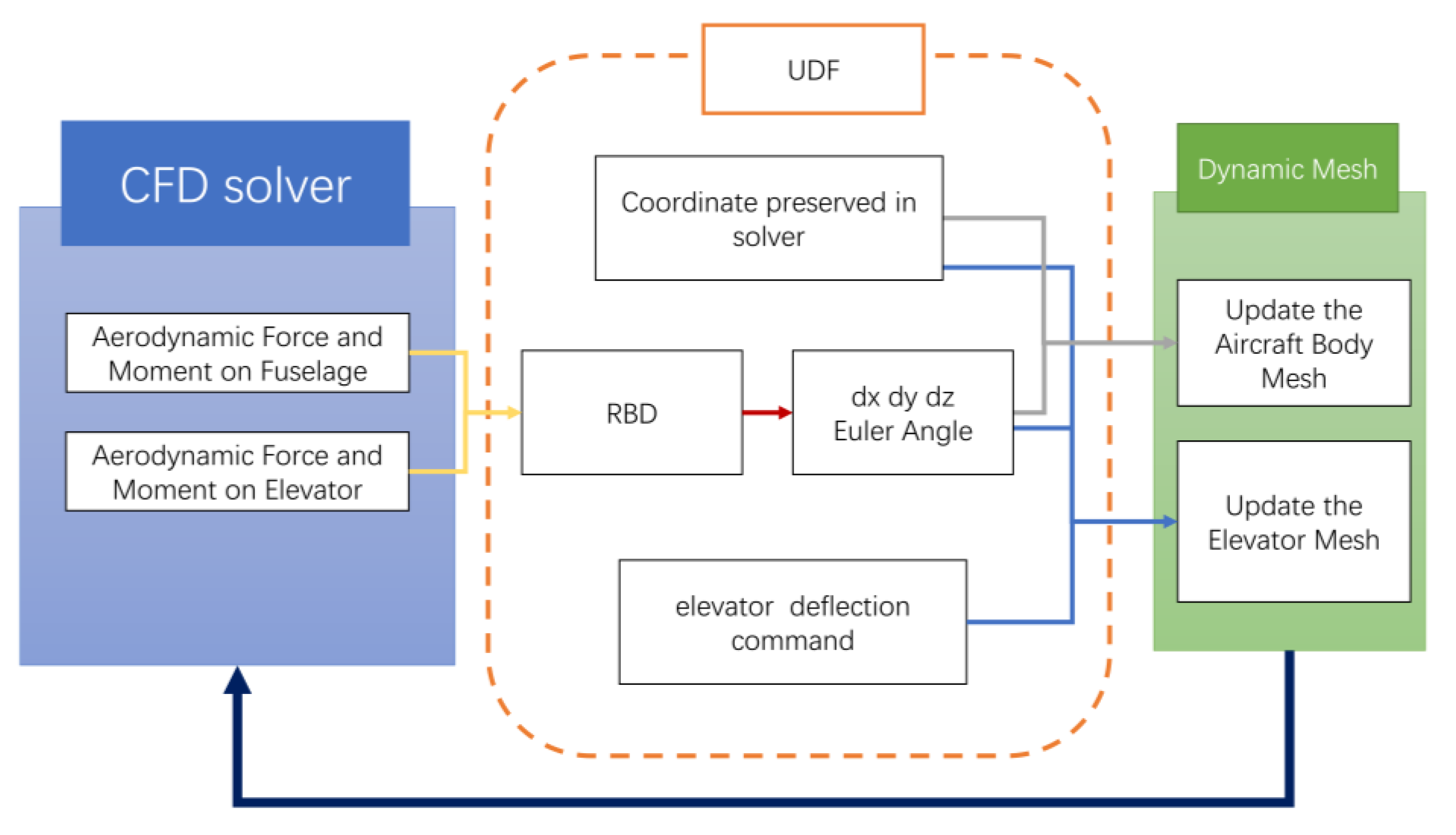
4.3. CFD/RBD Co-Simulation Procedure

This paper involves simulating the dynamic process of stimulating the short-period mode of aircraft by the deflection of the elevator, which requires that the aircraft body can realize the six-degree-of-freedom movement and the aircraft control surface can realize the deflection movement around the rotation axis according to the control instructions in the CFD environment.
Therefore, the boundary of the whole fluid calculation domain can be divided into three parts: the far field and the inner boundaries named fuselage and elevator, the latter two of which formed the aircraft aerodynamic model. The inner boundaries of the flow field are the moving boundaries by the motion of which the behavior of the aircraft body and elevator in the actual flow field is simulated.
The essence of the moving boundary is the update of the node coordinates of the mesh on the moving boundary of the fuselage and elevator (respectively, x f C , y f , C , z f , C and x e , C , y e , C , z e , C ) at each time step. In the RBD/CFD simulation calculation, the updating of coordinates of dynamic mesh is driven by the aircraft centroid position and attitude angle calculated by the flight dynamics calculation program in the RBD module. After the dynamic mesh is updated, the next round of CFD aerodynamic calculation and flight dynamics calculation is carried out. Through the above method, data coupling between the modules of CFD and RBD is generated, and the co-simulation of the two modules is realized.
The procedure flow is as shown in Figure 8: firstly, the aerodynamic computational mesh of RBD/CFD co-simulation in the initial state (time step = 0) is generated. The AOA and the elevator deflection angle of the aircraft aerodynamic model can refer to the results of the trim calculation carried out by AVL software under the same working conditions as the time domain co-simulation. The incoming flow direction is set to the x-axis of the reference frame in the computational fluid domain, so the initial pitch attitude angle of the aircraft should be equal to the trim AOA under the computational fluid reference frame. In addition, the position of the centroid of the aircraft should be made to coincide with the origin of the CFD frame and deflect the elevator dynamic boundary to the trim opening.
Second, node coordinates of the dynamic mesh of the fuselage and elevator relative to the body frame x f , B , y f , B , z f , B and x e , B , y e , B , z e , B were generated. The access of node coordinates of the fuselage and elevator relative to the CFD frame can be achieved by the UDF program first, and then the coordinates are transformed into x f , B , y f , B , z f , B and x e , B , y e , B , z e , B and stored in.csv files. The data in the CSV file are used to initialize the subsequent time domain simulation.
For the initialization of the program, the node coordinates of dynamic mesh on the fuselage and elevator relative to the body frame x f , B , y f , B , z f , B and x e , B , y e , B , z e , B are stored in the CFD solver as global variables. When the co-simulation goes to t time step, the pressure of each face element on the dynamic mesh of fuselage and elevator at t time step is obtained by CFD fluid solver, and the aerodynamic force and moment time step t can be obtained by summating the product of the pressure and area of every face element. Then, the aerodynamic force and moment are input into the RBD module.
After the RBD module receives the aerodynamic force obtained by the CFD solver, combined with state variables of flight dynamic equations of t time step, the position coordinates x c m , I , y c m , I , z c m , I and the attitude angles φ I , θ I , ψ I of aircraft on the t + 1 time step can be acquired by solving the flight dynamics equation in an inertial frame. By the transformation relation mentioned in the section on a coordinate system, the x c m , I , y c m , I , z c m , I and φ I , θ I , ψ I is transformed into x c m , C , y c m , C , z c m , C and φ C , θ C , ψ C , which are the centroid position and attitude angle of aircraft in the reference frame of the fluid computing domain.
The last step is to update the computing dynamic mesh. The coordinates of the node on fuselage dynamic mesh are updated first. The coordinates of a fluid node of fuselage dynamic mesh in the body frame x f , B , y f , B , z f , B are angular transformed by the angle of φ C , θ C , ψ C acquired in the last step and translated by x c m , C , y c m , C , z c m , C , by which the coordinates of the fluid node of fuselage dynamic mesh in the CFD frame x f , C , y f , C , z f , C are obtained. The next is to complete the dynamic mesh update of the elevator, which can be divided into two cases. When there is no elevator deflection command in t time step, that is, when the elevator is in a neutral position, the coordinates of a fluid node of the elevator dynamic mesh x e , B , y e , B , z e , B under the body frame can be transformed directly to x e , C , y e , C , z e , C according to the angle and displacement calculated by RBD. Additionally, if there is a deflection of the elevator, the transformation of the coordinates of the elevator relative to the body frame should be achieved first, by which the coordinates of the deflected elevator in the body frame could be obtained:
x e , l o c a l = x e , B x o , l o c a l y e , l o c a l = y e , B z e , l o c a l = z e , B z o , l o c a l x e , B = cos ( Δ δ e ) * x e , l o c a l sin ( Δ δ e ) * y e , l o c a l + x o , l o c a l y e , B = y e , B z e , B = sin ( Δ δ e ) * x e , l o c a l + cos ( Δ δ e ) * y e , l o c a l + y o , l o c a l
where x e , l o c a l , y e , l o c a l , z e , l o c a l are the coordinates of the elevator in the local reference frame, x o , l o c a l , y o , l o c a l , z o , l o c a l are the coordinates of the origin of the local reference frame relative to the body frame, x e , B , y e , B , z e , B is the coordinate of undeflected elevator dynamic mesh in the body frame and x e , B , y e , B , z e , B is the coordinate of deflected elevator dynamic mesh in the body frame, Δ δ e is the elevator deflection angle by command. Finally, just like the operation in the first case, the coordinates of the deflected elevator dynamic mesh in the body frame were transformed into the mesh of the elevator in the fluid computational frame.

4.4. Verification of RBD/CFD Co-Simulation

This paper verifies the validity of CFD/RBD coupling simulation by comparing the short-period poles that come from system identification based on RBD/CFD time domain simulation data with the short-period poles calculated by AVL’s nmode function. The time-domain simulation data involved in system identification include the AOA response curves to the elevator step input at four Mach numbers, as shown in Figure 9. The comparison of pole distribution is shown in Figure 10. It can be seen from the figure that the short-period pole distribution obtained by RBD/CFD co-simulation is similar to that obtained by AVL calculation, especially the natural frequency and the variation trend with Mach number are consistent, and there are only some errors in damping ratio.

5. Co-Simulation of CFD/CSD/RBD

5.1. Structural Model of HWB

Because the aerodynamic model used in CSD/CFD/RBD co-simulation is completely consistent with the model used in CFD/RBD simulation, the aerodynamic model is not described here; only the finite element structure model of the aircraft is introduced. The FEM model of the aircraft is shown in Figure 11.
Firstly, the finite element modeling of the fuselage is introduced. The finite element model of the fuselage is shown in the figure, including structural elements such as fuselage skin, cabin lattice frame, wing ribs, wing beam and wing skin. The entire finite element model has nearly 3189 finite elements, which can represent more than 10,300 degrees of freedom. Three- or four-node curved plate elements are used to approximate the structure of the skin, beam, etc. Frames are represented by bending bar elements. The wing fin is represented by an axial rod element. As for the material properties of the element, the material is divided into spar material and skin material with reference to the literature [32], and the external skin and internal structure are, respectively, assigned two types of structural properties.
Due to the relatively small size of the elevator, it is simplified to a rigid body model in the co-simulation. Moreover, the aircraft structure, except the elevator, is regarded as an elastic body. In order to avoid geometric interference between the rigid elevator and the elastic fuselage caused by fuselage deformation in the process of co-simulation, it is necessary to set some constraints on the structural model of the elastic fuselage: for the two walls of the fuselage near the control surface, a relatively rigid constraint should be applied on the corresponding finite element. Through this constraint, no relative movement of the two sides walls can be guaranteed, and a movement space with a fixed boundary can be provided for the motion of the elevator. The implementation method in this paper is to use RB2 constraints in the MPC function of MSC. Patran multi-point constraints to carry out relatively rigid constraints on the nodes on the fuselage wall near the elevator.
Based on the above finite element model, the first four-order elastic modes of aircraft can be obtained through modal analysis, and the mode shapes and natural frequencies are shown in Figure 12.

5.2. Procedure of Co-Simulation of CFD/CSD/RBD

The procedure of co-simulation of CFD/CSD/RBD is shown in Figure 13. Firstly, the simulation program was initialized: the CFD/CSD interface interpolation matrix, the aircraft structure modal shape matrix, and the coordinates of the fluid node of the dynamic mesh of fuselage and elevator in the body reference frame in the initial state were stored in the CFD solver in the form of global variables.
When the co-simulation goes to the t time step, the solution of the fluid dynamics is completed first. The CFD solver completes the transient analysis of the flow field according to the fluid computational mesh and the boundary conditions at this time step, and then the pressure distribution on the dynamic mesh of the fuselage and elevator is obtained. The pressure distribution on the fuselage is used in two aspects: On the one hand, the aerodynamic force and moment generated by the fuselage are obtained by summation of the product of pressure and area of each mesh element on the whole fuselage. The force and moment are input to the RBD module for the subsequent flight dynamics calculation. On the other hand, the pressure distribution on the dynamic mesh of the fuselage is transformed into the aerodynamic load distribution on the fluid node of the dynamic mesh of the fuselage and input to the CSD computing module. As for the pressure distribution on the elevator dynamic mesh, due to the rigid body assumption for the elevator, this part of the data only enters the RBD module but does not participate in the CSD calculation module.
After the completion of the CFD solution and the processing of the pressure on the dynamic mesh, the solution of the structure is calculated in the body frame, the ultimate goal of which is to obtain the coordinates of the fluid node of the dynamic mesh of deformed fuselage in the body frame x f , B , y f , B , z f , B . The aerodynamic load is distributed on each fluid node of the dynamic mesh of the fuselage, which could be transformed into the aerodynamic load distribution on the structural FEM node through the CFD/CSD interface interpolation. According to the load distribution and the state variables of the fuselage FEM node at the t time step, the displacement and velocity of the fuselage FEM node at the t + 1 time step can be calculated by the structural dynamics calculation program. The displacement of the FEM node could be transformed into the displacement of the fluid node of fuselage dynamic mesh relative to the body frame by the fluid/solid interface interpolation d x f , B , d y f , B , d z f , B . The coordinates of the fluid node are added to the body frame x f , B , y f , B , z f , B with the newly calculated displacements, the coordinates fluid node of the deformed fuselage dynamic mesh in the body frame x f , B , y f , B , z f , B can be obtained.
Then, there is the solution of aircraft flight dynamics. After the RBD module receives the aerodynamic force calculated by the CFD solver, combined with state variables of flight dynamic equations at a t time step, the position coordinates x c m , I , y c m , I , z c m , I and the attitude angles x c m , C , y c m , C , z c m , C of aircraft relative to the inertial frame at t + 1 time step can be calculated by solving the flight dynamics equation.
By the transformation relation mentioned in the section on the reference frame, the obtained variables above are transformed to the counterpart in the fluid computational reference frame x c m , I , y c m , I , z c m , I , φ I , θ I , ψ I .The last step of the co-simulation in the t time step is to update the dynamic mesh of the fuselage and elevator. This part is completely consistent with the mesh updating method of RBD/CFD co-simulation, except that the update of the dynamic mesh of the fuselage is based on the coordinates x f , B , y f , B , z f , B , which corresponds to the deformed fuselage relative to the body frame. After the update of the dynamic mesh, the co-simulation advances to the next time step.

5.3. Results of Co-Simulation of CFD/CSD/RBD

In this paper, the time domain simulation calculation based on CFD/CSD/RBD coupling under the condition of pulse input of elevator is completed, respectively, at 0.5, 0.6, 0.7 and 0.8 Mach numbers. Considering that the natural frequency of the elastic mode is close to that of the aircraft’s short-period mode, the elastic effect should have the most significant influence on the aircraft’s short-period mode. Therefore, the response curves of the angle of attack are selected as the display of the aircraft’s short-period characteristics in the calculation results of the four simulation groups (as shown in Figure 14).

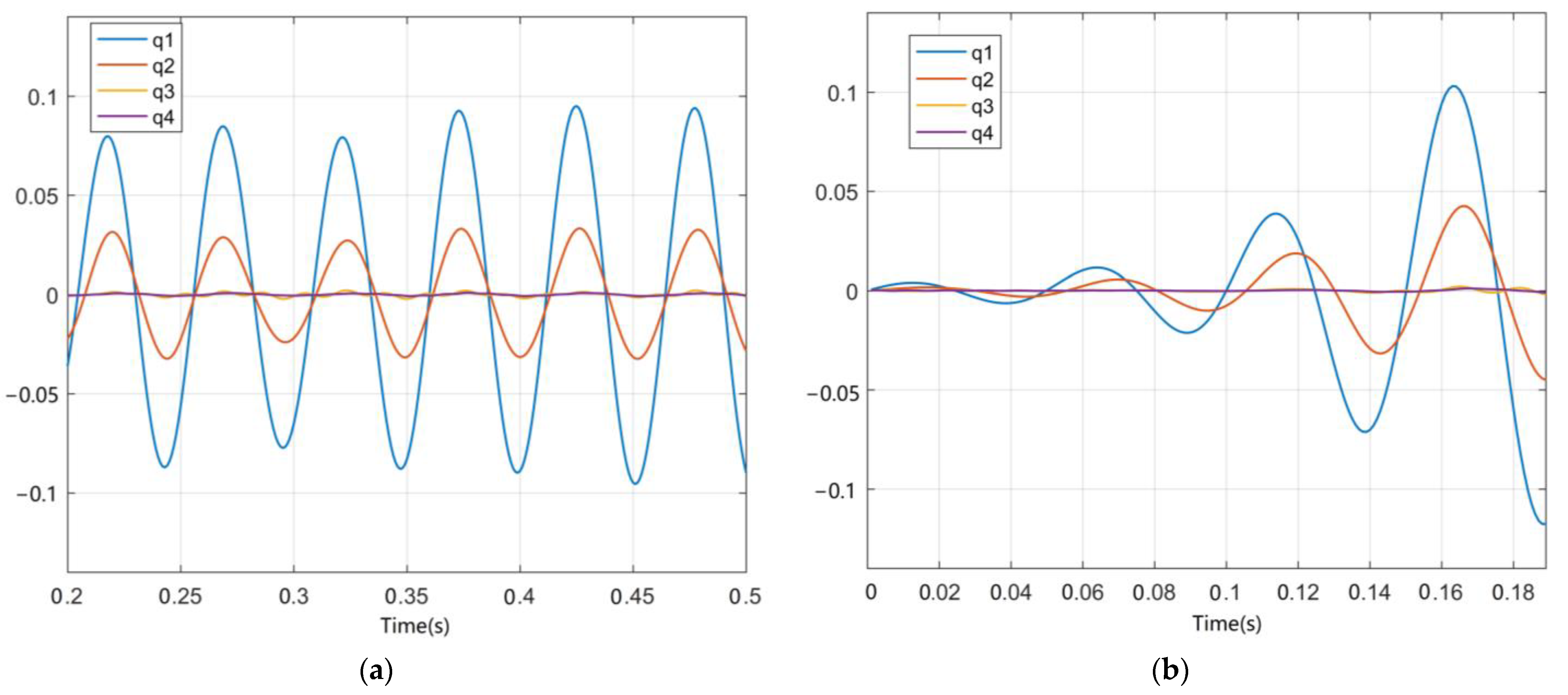
5.4. Discussion on the Results of Co-Simulation

According to Figure 14, as the Mach number increases, the response curve of the angle of the attack shows an increasing natural frequency and decreasing damping ratio, which is in accordance with the general trend of aircraft dynamics characteristics with increasing Mach number. The red dotted line represents the response curve taking into account the elastic effect of the aircraft structure, while the solid blue line represents the corresponding response of the angle of attack without the elastic effect. From the calculation results under each Mach number, it can be seen that the elastic effect makes the response curve slightly lag behind the rigid body case in phase, which is due to a decrease in natural frequency, while the amplitude narrows significantly compared with the rigid body case, and the above trends are in line with those of the theoretical calculations in the literature. Additionally, the final steady-state angle of attack also increases slightly compared with the rigid body case, and the above trend becomes more significant with the decrease in Mach number.

6. Conclusions

In this paper, a CFD/CSD/RBD co-simulation platform is developed, which integrates the CFD/CSD coupling calculation technology and the virtual flight technology based on the CFD/RBD coupling calculation, and the validity of the two kinds of calculation was verified, respectively. This platform can be used as an important tool for the subsequent research on the rigid–elastic coupled problems of flexible HWB aircraft. Then, by means of the co-simulation technology, this paper completed the time-domain flight simulation of HWB aircraft for the elevator pulse input under the conditions of 0.5, 0.6, 0.7 and 0.8 Mach number, respectively. Based on the series of simulations, the influence of the elastic effect on the short-period dynamic characteristics of HWB aircraft was studied. According to the simulation results, it is clear that the rigid–elastic coupling effect reduces the natural frequency of the short-period characteristics of the HWB aircraft and increases the damping ratio, and the rigid–elastic coupling effect causes more significant changes in the damping ratio than in the natural frequency. In addition to the effect on dynamic characteristics of HWB aircraft, this study found that rigid–elastic coupling effect also increases the trim angle of attack of the aircraft to a certain extent. For variation in both dynamic and steady-state characteristics mentioned above, it will be more significant with the decrease in Mach number.

Author Contributions

Y.W. performed the main work of this article, including the conception of this study, calculations, and manuscript writing; G.L. contributed significantly to the analysis of computations and the revision of this article. All authors have read and agreed to the published version of the manuscript.

Funding

This research received no external funding.

Institutional Review Board Statement

Not applicable.

Informed Consent Statement

Not applicable.

Data Availability Statement

No new data were created or analyzed in this study. Data sharing is not applicable to this article.

Conflicts of Interest

The authors declare no conflict of interest.

Nomenclature

HWBHybrid Wing Body
AOAAngle of Attack
CFDComputational Fluid Dynamics
CSDComputational Structure Dynamics
RBDRigid-Body Dynamics
RANSReynolds-averaged Navier–Stokes equations
MNMach Number
AVLAthena Vortex Lattice
FSIFlutter Speed Index
FEMFinite Element
UDFUser Defined Function
DLMDouble-let Lattice Method
Φ Matrix of Mode Shape
M Matrix of Mass
C Matrix of Damping
K Matrix of Stiffness
u , v , w Component of Velocity relative to body frame
p , q , r Component of Angular Velocity relative to body frame
ϕ Thin Plate Spline Basic Function
H Solid/Fluid Interface Interpolation Matrix
x c m , I , y c m , I , z c m , I Center of Mass of Aircraft in Inertial Frame
φ I , θ I , ψ I Attitude angle of Aircraft in Inertial Frame
x c m , c , y c m , c , z c m , c Center of Mass of Aircraft in CFD Frame
φ I , θ I , ψ I Attitude angle of Aircraft in CFD Frame
x f , C , y f , C , z f , C Coordinates of Fuselage Mesh in CFD Frame
x e , C , y e , C , z e , C Coordinates of Elevator Mesh in CFD Frame
x f , B , y f , B , z f , B Coordinates of Fuselage Mesh in body Frame
x e , B , y e , B , z e , B Coordinates of Elevator Mesh in body Frame
x f , B , y f , B , z f , B Coordinates of Deformed Fuselage Mesh in body Frame
x e , B , y e , B , z e , B Coordinates of deflected Elevator Mesh in body Frame
d x f , B , d y f , B , d z f , B Displacement on Coordinates of Fuselage Mesh in body Frame
Δ δ e Deflected Angle of Elevator

References

  1. Dorian, F.C.; Nicholas, H.R. HALE Multidisciplinary Design Optimization Part II: Solar-Powered Flying-Wing Aircraft. In Proceedings of the 2018 Aviation Technology, Integration, and Operations Conference, Atlanta, GA, USA, 25–29 June 2018. [Google Scholar]
  2. Daniel, P.; Simon, B. The Integration of an Efficient High Lift System in the Design Process of a Blended Wing Body Aircraft. In Proceedings of the 12th AIAA Aviation Technology, Integration, and Operations Conference, Indianapolis, IN, USA, 17–19 September 2012. [Google Scholar]
  3. Melike, N.; Bret, S. Impact of Aeroelastic Uncertainties on the Sonic Boom Signature of a Commercial Supersonic Transport Configuration. In Proceedings of the AIAA Scitech 2017 Forum, Grapevine, TX, USA, 9–13 January 2017. [Google Scholar]
  4. Molong, D.; Carlos, E. Nonlinear Control-oriented Modeling for Very Flexible Aircraft. In Proceedings of the AIAA Scitech 2021 Forum, Virtual Event, 11–15 & 19–21 January 2021. [Google Scholar]
  5. Wang, X.R.; Tigran, M. Nonlinear Incremental Control for Flexible Aircraft Trajectory Tracking and Load Alleviation. J. Guid. Control Dyn. 2022, 45, 39–57. [Google Scholar] [CrossRef]
  6. Flávio, J.S.; Antônio, B.G. Aircraft Control Based on Flexible Aircraft Dynamics. J. Aircr. 2018, 54, 262–271. [Google Scholar]
  7. Wu, Z.G.; Yang, C. Flight Loads and Dynamics of Flexible Air Vehicles. Chin. J. Aeronaut. 2004, 17, 17–22. [Google Scholar] [CrossRef] [Green Version]
  8. Frank, G. Finite Element Based HWB Centerbody Structural Optimization and Weight Prediction. In Proceedings of the 53rd AIAA/ASME/ASCE/AHS/ASC Structures, Structural Dynamics and Materials Conference, Honolulu, HI, USA, 23–26 April 2012. [Google Scholar]
  9. Cai, Y.; Xie, J.C. Assessment of Longitudinal Stability-and-Control Characteristics of Hybrid Wing Body Aircraft in Conceptual Design. In Proceedings of the AIAA Aviation 2021 Forum, Virtual Event, 2–6 August 2015. [Google Scholar]
  10. Mardanpour, P.; Richards, W.P.; Nabipour, O.; Hodges, D.H. Effect of Multiple Engine Placement on Aeroelastic Trim and Stability of Flying Wing Aircraft. J. Fluids Struct. 2014, 44, 67–86. [Google Scholar] [CrossRef]
  11. Mardanpour, P.; Hodges, D.H.; Neuhart, R.; Graybeal, N. Engine Placement Effect on Nonlinear Trim and Stability of Flying Wing Aircraft. J. Aircr. 2013, 50, 1716–1725. [Google Scholar] [CrossRef]
  12. Giulio, A.; Francesco, N. Reduced-Order Short-Period Model of Flexible Aircraft. J. Guid. Control Dyn. 2017, 40, 2017–2029. [Google Scholar]
  13. Xie, C.C.; Yang, L. Stability of Very Flexible Aircraft with Coupled Nonlinear Aeroelasticity and Flight Dynamics. J. Aircr. 2018, 55, 862–874. [Google Scholar]
  14. Antônio, B.G.; Guilherme, C. Flexible Aircraft Simulation Validation with Flight Test Data. AIAA J. 2021, 61, 1–20. [Google Scholar]
  15. Antônio, B.G.; Roberto, G.A. Formulation of the Flight Dynamics of Flexible Aircraft Using General Body Axes. J. Aircr. 2016, 54, 3517–3534. [Google Scholar]
  16. Lars, R.; Markus, R. CFD-based Gust Load Analysis for a Free-flying Flexible Passenger Aircraft in Comparison to a DLM-based Approach. In Proceedings of the AIAA Aviation 2015 Forum, Dallas, TX, USA, 22–26 June 2015. [Google Scholar]
  17. Gul, D.; Altan, K. Aeroelastic Model Corrections of a Very Light Aircraft; Implications on Static Trim, Flutter and Gust Response. In Proceedings of the AIAA Aviation 2022 Forum, Chicago, IL, USA, 27 June–1 July 2022. [Google Scholar]
  18. Michele, C.; Jonathan, E.C. Nonlinear Static Aeroelasticity of High-Aspect-Ratio-Wing Aircraft by Finite Element and Multibody Methods. J. Aircr. 2017, 54, 548–560. [Google Scholar]
  19. Thiemo, M.K.; Bret, S. Comparison of Unsteady Aerodynamic Modelling Methodologies with Respect to Flight Loads Analysis. In Proceedings of the AIAA Atmospheric Flight Mechanics Conference and Exhibit, San Francisco, CA, USA, 9–13 August 2005. [Google Scholar]
  20. Pau, C.M.; Christophe, P. Simulation of Flexible Aircraft Response to Gust and Turbulence for Flight Dynamics Investigations. In Proceedings of the AIAA Scitech 2020 Forum, Orlando, FL, USA, 6–10 January 2020. [Google Scholar]
  21. Martin, L.; Andreas, K. Flight Dynamics Modeling of a Body Freedom Flutter Vehicle for Multidisciplinary Analyses. In Proceedings of the AIAA Scitech 2015 Forum, Kissimmee, FL, USA, 5–9 January 2015. [Google Scholar]
  22. Ethan, C.; Matthew, F. Transient CFD/CSD Tiltrotor Stability Analysis. In Proceedings of the AIAA Scitech 2019 Forum, San Diego, CA, USA, 7–11 January 2019. [Google Scholar]
  23. Amine, A.; Muhammed, K.Y. CFD/CSD Coupling for Camber Morphed Rotor Blades. In Proceedings of the AIAA Aviation 2022 Forum, Chicago, IL, USA, 27 June–1 July 2022. [Google Scholar]
  24. Chen, G.; Zhou, Q. Computational-Fluid-Dynamics-Based Aeroservoelastic Analysis for Gust Load Alleviation. J. Aircr. 2018, 55, 1620–1628. [Google Scholar] [CrossRef] [Green Version]
  25. Amin, F.; Anant, G. Computational Aeroelastic Analysis using an Enhanced OpenFOAM-based CFD-CSD Solver. In Proceedings of the 2018 AIAA/ASCE/AHS/ASC Structures, Structural Dynamics, and Materials Conference, Kissimmee, FL, USA, 8–12 January 2018. [Google Scholar]
  26. Nidhi, D.S.; Klaus, A.H. Trajectory Prediction Using Coupled CFD-RBD with Dynamic Meshing. In Proceedings of the AIAA Scitech 2019 Forum, San Diego, CA, USA, 7–11 January 2019. [Google Scholar]
  27. Jubaraj, S.; Frank, F. Computational and Experimental Free-Flight Motion of a Subsonic Canard-Controlled Body. In Proceedings of the AIAA Aviation 2017 Forum, Denver, CO, USA, 5–9 June 2017. [Google Scholar]
  28. Cui, P.; Han, J.L. Numerical investigation of the effects of structural geometric and material nonlinearities on limit-cycle oscillation of a cropped delta wing. J. Fluids Struct. 2011, 27, 611–622. [Google Scholar]
  29. Wang, N.H.; Ma, R. Numerical Virtual Flight Simulation of Quasi-Cobra Maneuver of a Fighter Aircraft. J. Aircr. 2021, 58, 139–152. [Google Scholar] [CrossRef]
  30. Zhang, L.P.; Zhao, Z.L.; Chang, X.H. Validation of Numerical Virtual Flight System with Wind-Tunnel Virtual Flight Testing. AIAA J. 2020, 58, 1566–1579. [Google Scholar]
  31. Carson, Y. AGARD Standard Aeroelastic Configurations for Dynamic Response I-Wing 445.6; NASA Langley Research Center: Hampton, VA, USA, 1988. [Google Scholar]
  32. Victor, L.; Kim, L. Hybrid Wing Body (HWB) Aircraft Design and Optimization Using Stitched Composites. In Proceedings of the AIAA Aviation 2015 Forum, Dallas, TX, USA, 22–26 June 2015. [Google Scholar]
Figure 1. Program structure of the CFD/CSD/RBD co-simulation.
Applsci 13 00410 g001
Figure 2. Procedure of CFD/CSD simulation.
Applsci 13 00410 g002
Figure 3. Geometric parameters of AGARD 445.6 Wing.
Applsci 13 00410 g003
Figure 4. FEM model of AGARD 445.6 Wing.
Applsci 13 00410 g004
Figure 5. CFD mesh of AGARD 445.6 Wing.
Applsci 13 00410 g005
Figure 6. The flutter boundary calculated in this paper are compared with the experimental results [31].
Applsci 13 00410 g006
Figure 7. Time-domain responses of AGARD 445.6 wing at Mach 0.678: (a) FSI = 0.407; (b) FSI = 0.417.
Applsci 13 00410 g007
Figure 8. Program procedure of the CFD/RBD co-simulation.
Applsci 13 00410 g008
Figure 9. The AoA response of aircraft at different Mach numbers based on CFD/RBD co-simulation.
Applsci 13 00410 g009
Figure 10. Poles of short-period mode calculated by AVL and CFD method.
Applsci 13 00410 g010
Figure 11. The FEM model of HWB aircraft.
Applsci 13 00410 g011
Figure 12. The mode shape of first four modes of HWB aircraft: (a) Mode 1, Freq = 1.15 Hz; (b) Mode 2, Freq = 1.58 Hz; (c) Mode 3, Freq = 4.22 Hz; (d) Mode 4, Freq = 4.75 Hz.
Applsci 13 00410 g012
Figure 13. Program procedure of the CFD/CSD/RBD co-simulation.
Applsci 13 00410 g013
Figure 14. Response of AoA to the impulse input of elevator based on CFD/CSD/RBD co-simulation.
Applsci 13 00410 g014aApplsci 13 00410 g014b
Table 1. Material Properties of AGARD 445.6 Wing.
Material PropertiesValue
Longitudinal Young’s modulus3.1511 Gpa
Lateral Young’s modulus0.4162 Gpa
Poisson’s ratio0.31
Density381.98 kg/m3
Table 2. Comparison of experimental and calculated natural frequencies of the first four modes.
Mode 1Mode 2Mode 3Mode 4
Experiment9.638.150.798.5
Simulation8.839.451.6100.8
Disclaimer/Publisher’s Note: The statements, opinions and data contained in all publications are solely those of the individual author(s) and contributor(s) and not of MDPI and/or the editor(s). MDPI and/or the editor(s) disclaim responsibility for any injury to people or property resulting from any ideas, methods, instructions or products referred to in the content.

