Retinal Nerve Fiber Layer Analysis Using Deep Learning to Improve Glaucoma Detection in Eye Disease Assessment

Abstract

Recently, the development of a rapid detection approach for glaucoma has been widely proposed to assist medical personnel in detecting glaucoma disease thanks to the outstanding performance of artificial intelligence. In several glaucoma detectors, cup-to-disc ratio (CDR) and disc damage likelihood scale (DDLS) play roles as the major objects that are used to analyze glaucoma. However, using CDR and DDLS is quite difficult since every person has different characteristics (shape, size, etc.) of the optic disc and optic cup. To overcome this issue, we proposed an alternative way to detect glaucoma disease by analyzing the damage to the retinal nerve fiber layer (RNFL). Our proposed method is divided into two processes: (1) the pre-treatment process and (2) the glaucoma classification process. We started the pre-treatment process by removing unnecessary parts, such as the optic disc and blood vessels. Both parts are considered for removal since they might be obstacles during the analysis process. For the classification stages, we used nine deep-learning architectures. We evaluated our proposed method in the ORIGA dataset and achieved the highest accuracy of 92.88% with an AUC of 89.34%. This result is improved by more than 15% from the previous research work. Finally, it is expected that our model could help improve eye disease diagnosis and assessment.

1. Introduction

Glaucoma is a chronic eye disease estimated to be the second leading cause of blindness globally. It is indicated by the degeneration of optic fiber, which leads to gradual optic nerve damage [1,2]. The number of glaucoma patients reached 80 million in 2020, in which, approximately 50% of people affected by glaucoma are unaware of this eye disease [3]. Irreversible vision loss will occur if the patients are not treated properly. Hence, early screening and gradual proper treatment are necessary to avoid vision loss and to retard the progression of glaucoma disease [4].

Traditionally, the glaucoma early screening procedure is conducted by calculating and analyzing the value of the cup-to-disc ratio (CDR) and disc damage likelihood scale (DDLS) [3,5]. CDR and DDLS values are the gold standards in diagnosing glaucoma, which define the ratio between the optic cup and optic disc and consist of some range that indicates the level of the damage [3]. To calculate CDR and DDLS, the doctor needs to measure some parameters, such as the diameter of the optic disc (OD) and optic cup (OC), the angle of the optic cup, and the closest distance between the optic cup and optic disc. OD and OC become the major objects used to calculate CDR and DDLS since the degeneration of optic fiber gives a direct effect on the neural rhyme, which enlarges the optic cup area. According to this situation, the optic cup becomes larger than the optic disc, which changes the value of CDR and DDLS [3] (see Figure 1a,b). In addition to this screening procedure, the doctor often uses alternative procedures by analyzing the damage to the retinal nerve fiber layer (RNFL) [5,6]. The progressive damages to the RNFL are indicated by the loss of nerve fiber around the optic nerve head (ONH). This progressive damage can be relatively well-defined as a texture change in the retinal images (see Figure 1c). An example image in Figure 1c represents the RNFL loss around the optic disc and blood vessel, with an average result of the green and blue channels. Accentually, red green blue (RGB) color space cannot illustrate the RNFL clearly, hence, a different color space or channel should be utilized in an image [6].

In the glaucoma early screening procedure, the calculation and analysis of CDR, DDLS, and RNFL are conducted manually, which needs an expert, more time, and thoroughness of result. As an alternative, several researchers have developed a computer-aided diagnosis (CAD) to assist doctors in diagnosing glaucoma, and to be an alternative solution for the screening process, which needs a large amount of data to be examined. Recently, the machine learning approach became one of the solutions for developing CAD for glaucoma. As proposed by Lu et al. [7], 52 patients consisting of 20 with glaucoma and 32 healthy were classified into two classes by using four classifiers: linear logistic regression, support vector machine (SVM), random forest classifier, and gradient boosting classifier. Their proposed method successfully achieved an accuracy of 98.3%. Thangaraj and Natarajan [8] proposed a classification model for glaucoma by using a support vector machine. Other automated detection methods for glaucoma also have been researched using several machine-learning methods [9,10,11,12].

Regardless of enthusiasm for machine learning performance, it seems unadaptable, particularly for this big dataset. As a solution, a deep learning approach has been implemented in the development of CAD for glaucoma. Deep learning (DL) is a powerful learning model that has been widely used in some field studies, especially those which have complex behavior that can be solved with traditional machine learning. Despite the DL model having higher computational time and complexity than the machine learning approach, DL provides robust results, particularly in the big dataset. Several studies also reported that DL can be used to build a high-performance prediction model in many areas such as agriculture [13], manufacturing [14], and even behavioral science [15].

The various DL-based approaches are also widely used in the image analysis field. In the studies related to eye image analysis for glaucoma detection, Raghavendra et al. [16] applied eighteen layers of a convolutional neural network (CNN) on the 1426 images (589: normal and 837: glaucoma). Their method successfully attained an accuracy of 98.13%, a sensitivity of 98%, and a specificity of 98.3%. Vinícius dos Santos Ferreira et al. [17] applied a convolutional neural network to the classification model starting with the segmentation of the optic disc. Their proposed method was performed on the RIM-ONE, DRIONS-DB, and DRISHTI-GS databases and achieved 100% on all metrics by using the red channel of RGB. Another convolutional neural network for glaucoma classification was proposed by Al-Bander et al. [18]. Their study performed a fully automated system based on the CNN model without using other methods. Another researcher [19] performed a transfer learning method called ImagedNet to distinguish normal and glaucoma images. Their proposed method was performed on 277 normal data samples and 170 glaucomas and achieved an accuracy of 92.3% in the training process and 80% in the testing process. Phasuk et al. [20] applied a convolutional neural network on the ORIGA-650, RIM-ONE R3, and DRISHTI-GS datasets and achieved an area under the curve (AUC) of 0.94.

According to some previous studies of both machine learning and deep learning approaches, we concluded that OD and OC were the major objects used to classify the healthy and glaucomatous eyes based on images, which means that most of the previous research works focused on the CDR and DDLS characteristics. However, traditionally, it was difficult to ensure that the optic cup was enlarged as an indication of glaucoma, because every person may have a different characteristic of the optic disc. Hence, other solutions may have better potential to increase the accuracy of glaucoma assessment.

The performance of the DL-based model can also be enhanced by applying data treatment/pre-processing steps, as reported in earlier studies, in many applications, such as for human activity recognition [21], breast cancer classification [22], and dental biometrics [23]. Therefore, in this study, we suggested that applying data preprocessing will help in improving the performance of glaucoma detection/classification.

Besides analyzing the optic disc and optic cup, glaucoma can also be recognized by analyzing the damage to the retinal nerve fiber layer. The progression of the damage was easier to recognize by measuring the thickness of the retinal nerve fiber layer. According to a medical report [24], analyzing the thickness of the retinal nerve fiber layer was a more objective and reliable method for assessing the possibility of glaucoma. They also said that analyzing the progress of the retinal nerve fiber layer was extremely impactful in the disease monitoring process. Regarding those facts, we proposed an effective solution for detecting glaucoma by analyzing the characteristic of the retinal nerve fiber layer. To address the research gaps, we presented the contributions including:

(i)

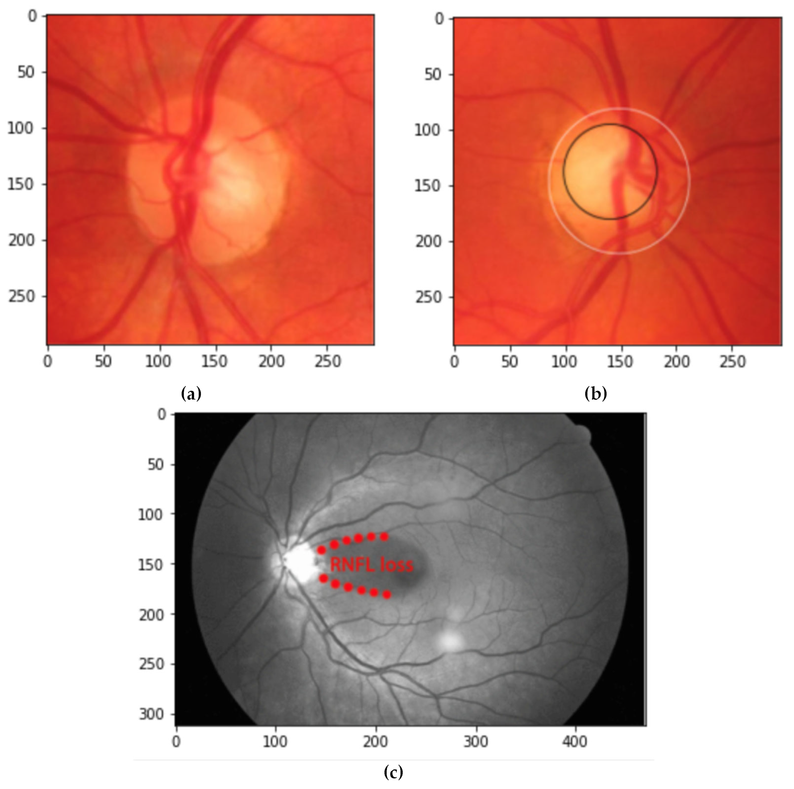
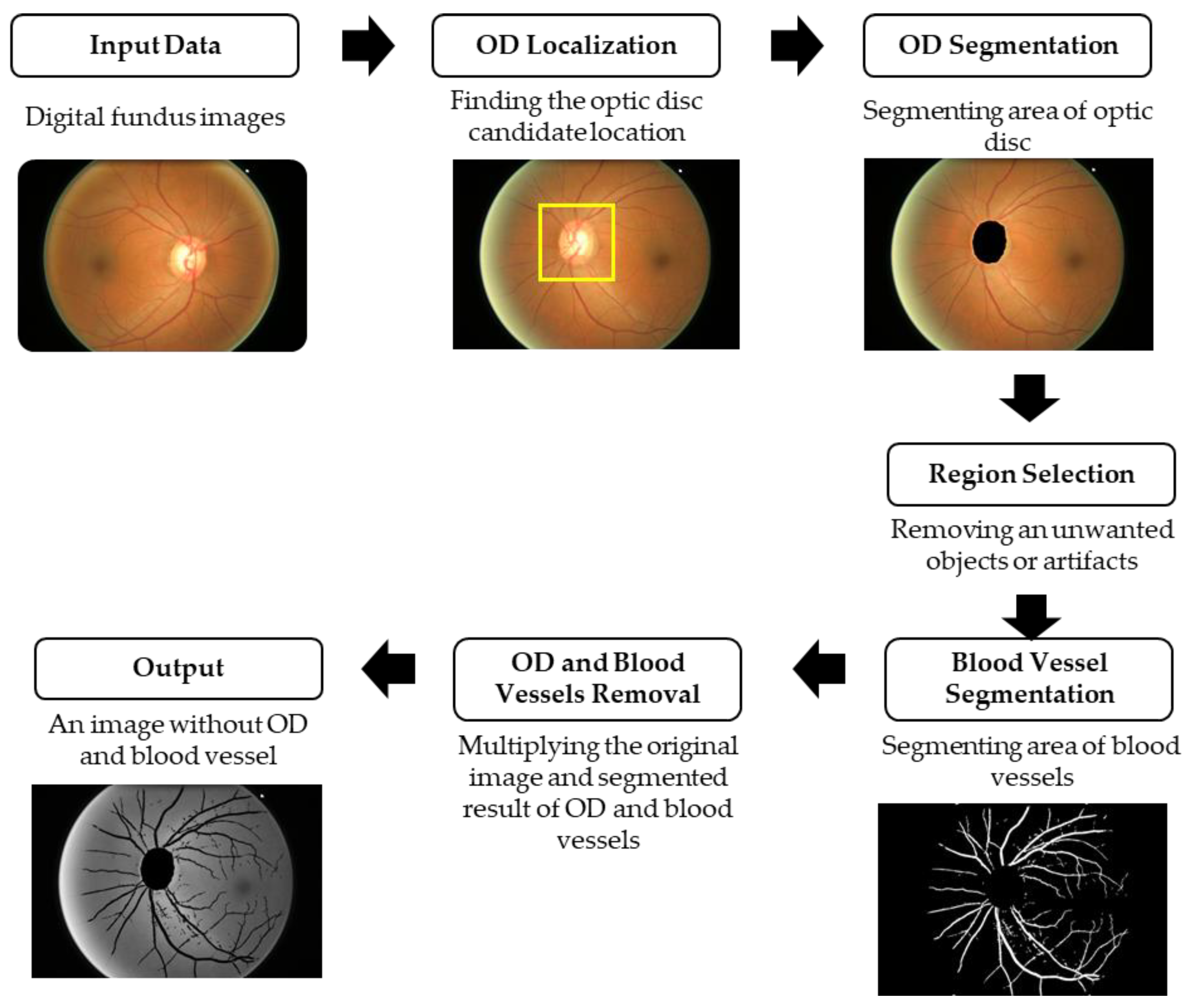
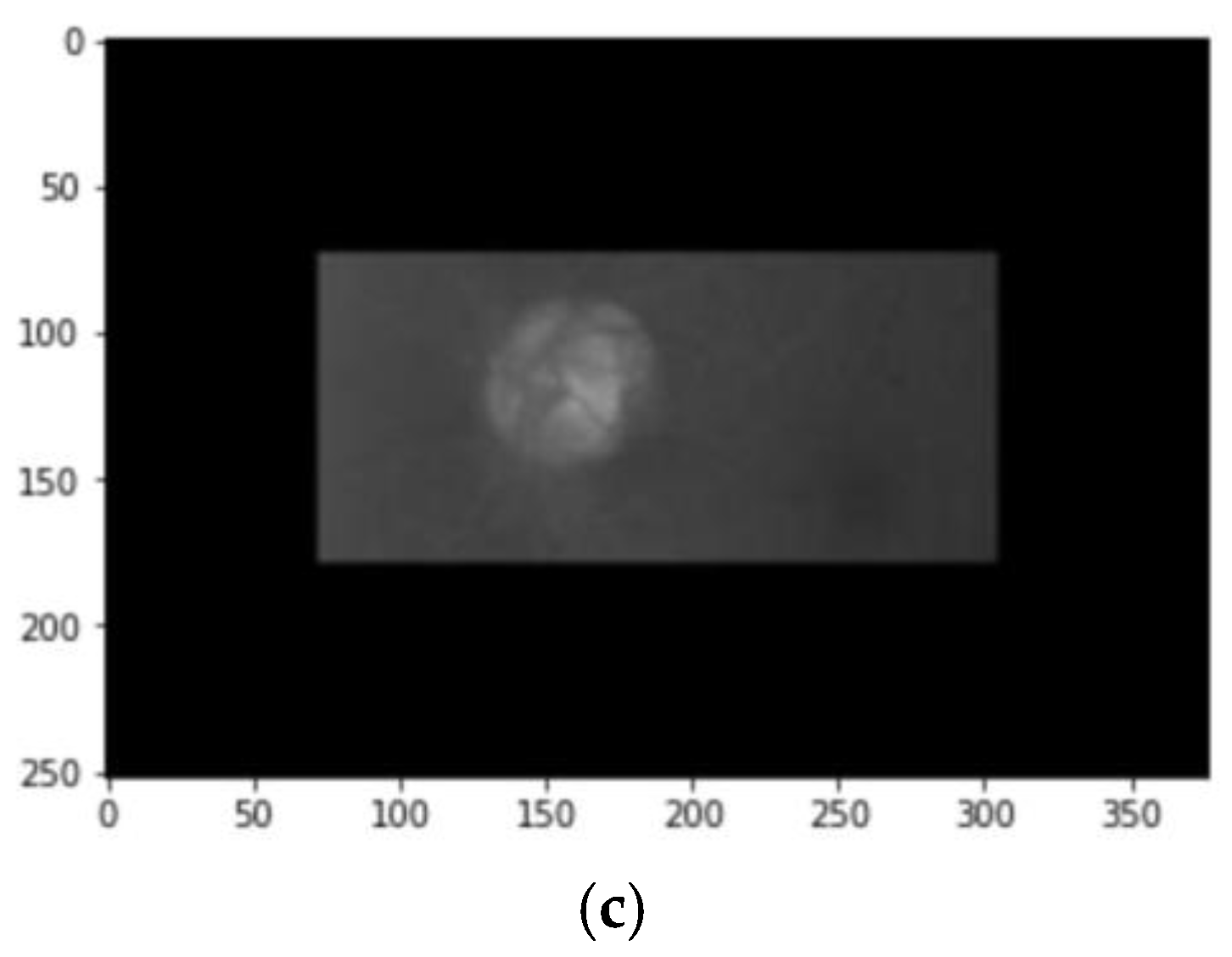
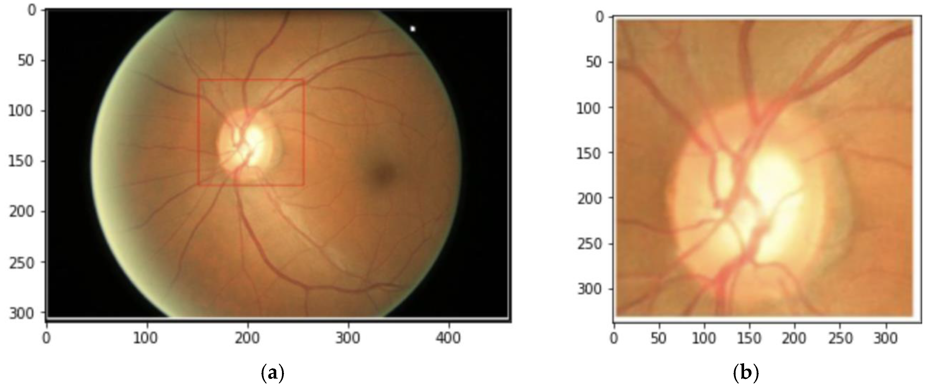
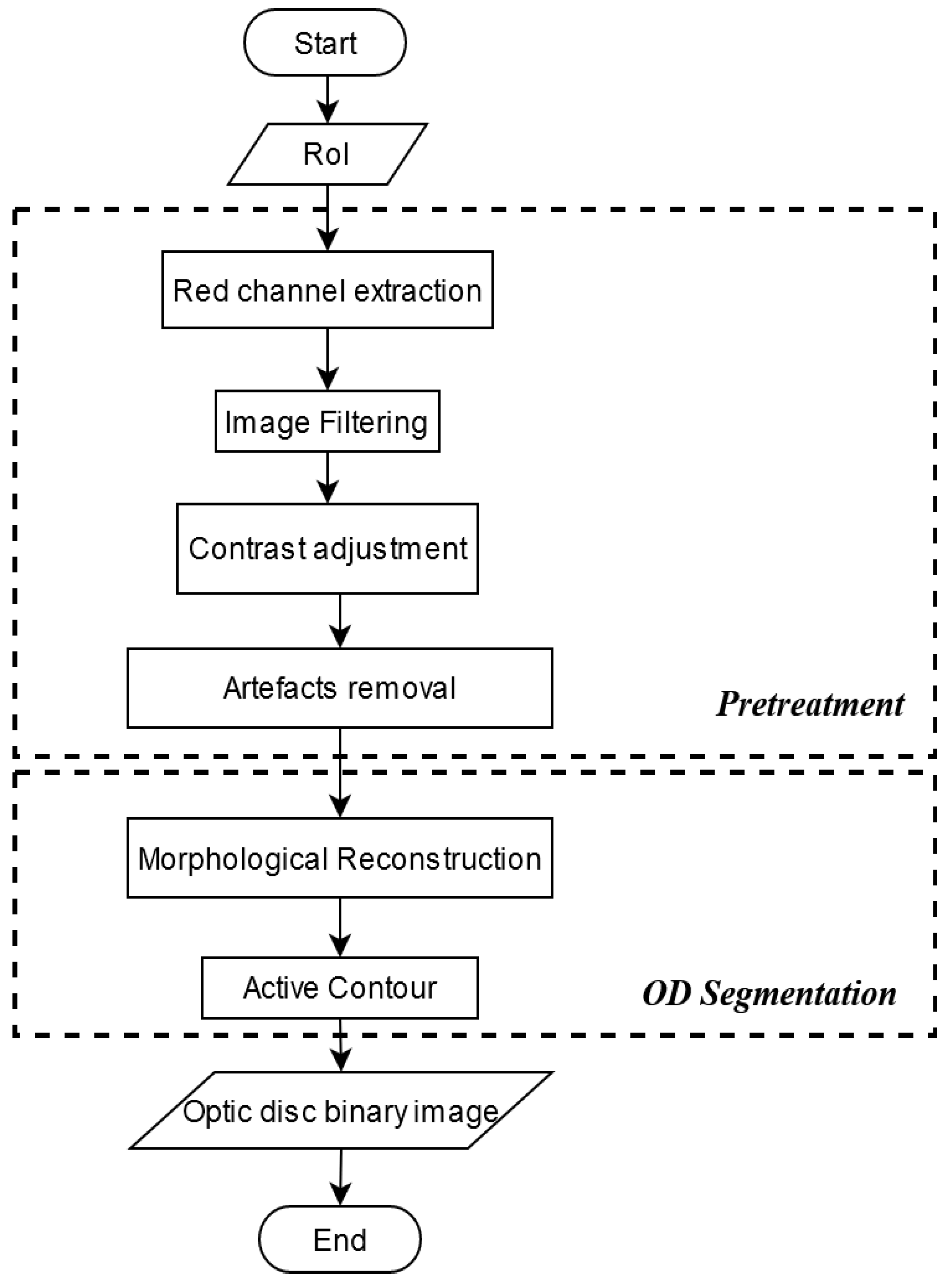
We proposed an alternative way to detect glaucoma disease by analyzing the damage to the retinal nerve fiber layer (RNFL). Our proposed method consists of novel step-by-step preprocesses to extract RNFL features from digital fundus images.

(ii)

We further analyze our methods by applying them in ORIGA dataset with nine pre-trained CNN and compared them with similar earlier studies about glaucoma classification which used the same dataset.

(iii)

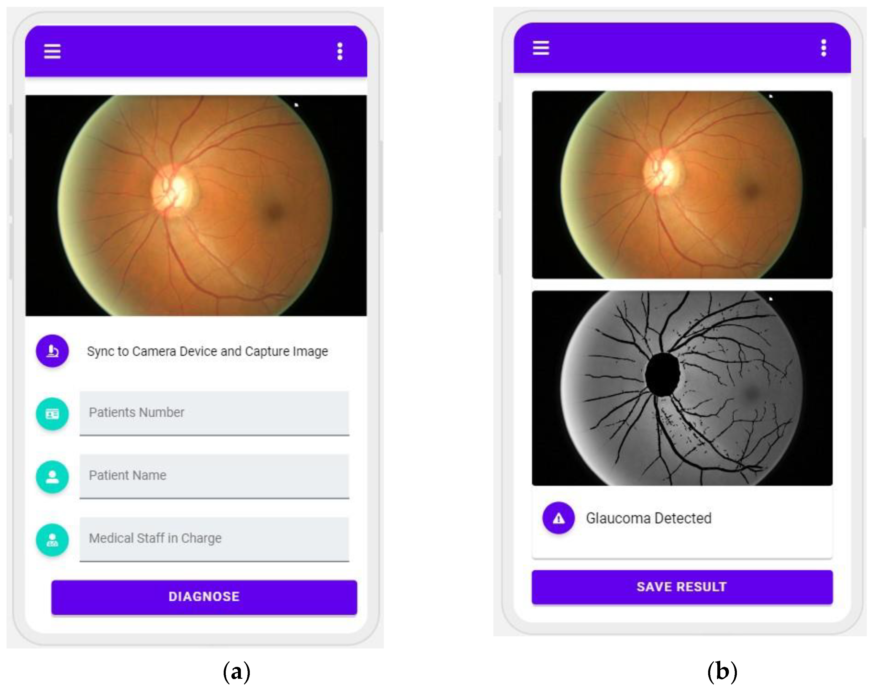
Finally, we developed a prototype application to categorize fundus images in order to demonstrate the viability of our proposed model. The designed and developed application is expected to be valuable for practitioners and decision-makers as practical guidelines for glaucoma detection and classification.

The remainder of this research is structured as follows. The materials and methods are presented in Section 2, including the dataset description, proposed method, data pre-processing, and experimental and DL model settings used in this research. Section 3 provides the experimental results and a comparison with the similar scenario in earlier works. Discussion and comparison with earlier works are presented in Section 4. Section 5 presents the conclusion, including future research directions. Finally, the list of abbreviations used in this research is provided in the Abbreviations section.

2. Materials and Methods

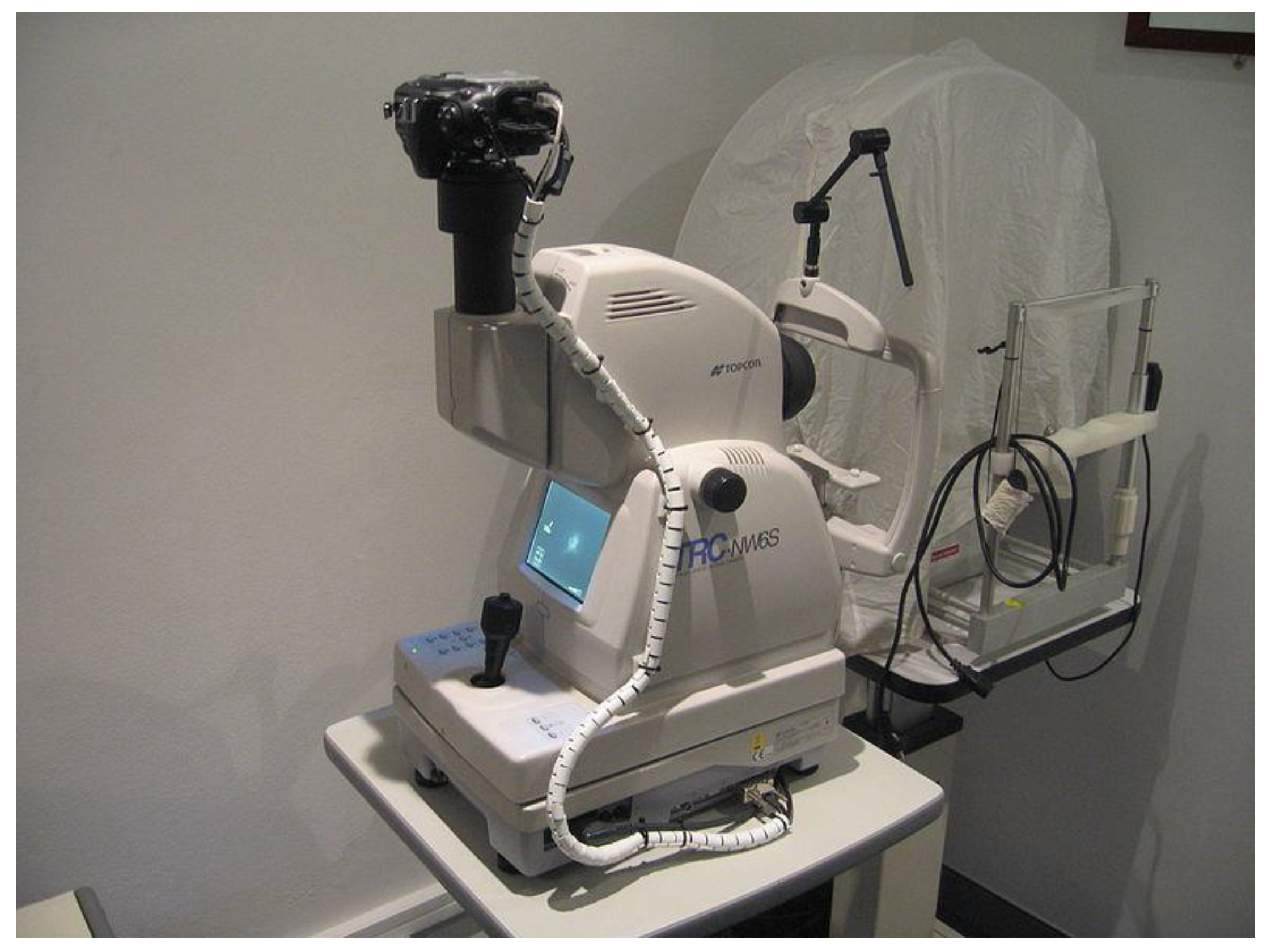
Generally, our proposed method consisted of four major processes, as shown in Figure 2. The four processes were the pre-processing step, data augmentation, glaucoma classification using several deep learning architectures, and evaluation process. We first describe the dataset used in this experiment, then, all steps are described in the following subsection.

2.1. Dataset

Developing an automated glaucoma detection system requires a lot of data to be trained. In this study, we used the ORIGA-light public dataset provided [25], which contained 650 images and was equipped with OD and OC ground truth, classification ground truth, CDR value, and diameter of OD. The ORIGA-light dataset provided 168 glaucomatous images and 482 healthy images.

Table 1. Characteristic of ORIGA-light dataset.

Component	Description
Case of dataset	Glaucoma
Type of data	RGB image
Dimension of data	3072 by 2048 pixel
Availability	Online access in [19]
Number of classes	2 classes (normal and glaucomatous)
Ground truth information	CDR value, segmentation ground truth of OD and OC, classification ground truth (normal and glaucomatous classes)
Number of data in each class	168 glaucomatous images and 482 healthy images

illustrates the summary of the dataset used in our study.

The ORIGA-light dataset has been studied intensively for several years and has produced various successes. As summarized in

Table 2. Recent studies in using ORIGA-light dataset.

Scope of Research	Researcher
Optic disc and optic cup localization and segmentation	[26,27,28,29,30,31,32,33,34,35,36]
Classification of glaucoma disease	[20,37,38,39,40,41]
Glaucoma detection	[42,43,44,45,46]
CDR estimation	[47]
Explainable or interpretable AI for glaucoma detection	[48,49]

, several researchers used the ORIGA-light dataset in three ways, i.e., (1) analyzing the presence of glaucoma using CDR value; (2) segmenting the OD and OC; (3) recognizing the glaucoma damage using the characteristics of OD and OC. However, most of the studies only focus on image segmentation parts rather than glaucoma detection and classification. Therefore, in our study, we proposed an alternative method to detect glaucoma disease by analyzing the damage to the retinal nerve fiber layer (RNFL).

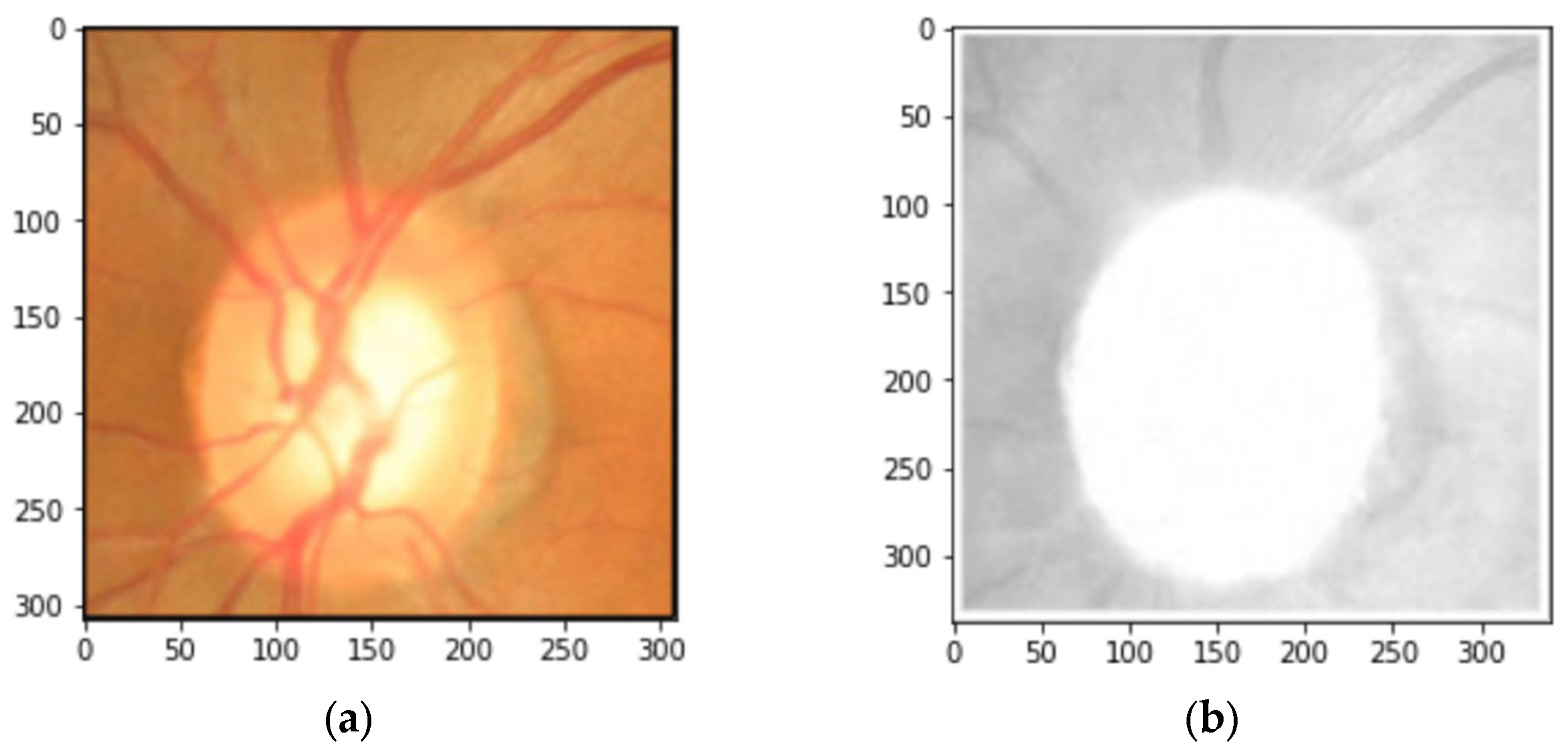
2.2. Data Preprocessing

In the pre-processing step, we focused on developing an image-processing technique that can delineate the characteristics of RNFL. RNFL is located around blood vessels and also close to the OD. As illustrated in Figure 1, the occurrence of RNFL was not clear, as there were blood vessels and OD in the way. Hence, we analyzed the RGB color space by separating every color channel and took a closer look into each of them. Finally, we found that the green channel of the RGB color space delineated the RNFL clearly. However, OD and blood vessels might still become an obstacle in the analysis process. Hence, in this step, we performed an OD and blood vessel removal scheme. The complete steps of the scheme are illustrated in Figure 3. As illustrated in Figure 3, the first step that is conducted in our experiment is OD and blood vessel removal. This process is carried out by conducting OD and blood vessel segmentation. The first important step before beginning the segmentation step is to locate the optic disc or optic nerve. This step is necessary to eliminate any peripheral area and merely focus on the optic nerve area.

In addition to Figure 3, Figure 4 illustrates the proposed technique of optic disc localization. Optic disc localization is conducted by first creating frames for every side of the input image. The frame width is 600 pixels from the peripheral to the center of the image, as shown in Figure 5b. This frame is useful to avoid the bright fringes around the retinal image. The bright fringe shown in Figure 5a is an area with a resemblance to the optic disc in terms of intensity value. A large area of the fringe can be mistaken as the optic disc, thereby leading to lower accuracy of localization. Hence, the RGB images need to subsequently be converted into a gray image by only taking the green channel. Then, this gray image can proceed to the next step. Since the dataset used in this experiment contained RGB images, we need to remove two channels and retain the other one. Because OC and OD may be seen in the green channel with more clarity than in the other two channels, the green channel is kept while the other two channels are discarded. Figure 6 illustrates the differences between each channel. Figure 6a illustrates an image of a red channel, Figure 6b illustrates an image of a green channel, and Figure 6c illustrates an image of a blue channel. According to these pictures, we can see that the image of the green channel appears clearer than other channels.

To yield a coherent RoI (region of interest) of the optic disc, searching for the center point is necessary. The search is conducted automatically by utilizing every column of the gray image’s matrix to find the highest pixel value. In Algorithm 1, I, queue, Total_Column, val, Idx represent the gray image, array lists containing the index of val, the number of columns of the gray image, the maximum intensity value of the current column, and the index of the maximum intensity value, respectively.

Algorithm 1. The search for the highest pixel value from every column of the image.

1: input: given I

2: given queue

3: for n = 1 to Total_Column do

4:  val = maximum value of $I_n$

5:  Idx = index of val

6:    If val ≥ 100 then

7:  store Idx to queue

8: end if

9: end for

If there is more than one highest value found in the column, only the value with the least index number can proceed to the conditional process. Based on our empirical experiment, generally, the pixel intensity inside the optic disc is above 100 (inside the green channel). Hence, we define 100 as the threshold. Once the desired indexes are gathered and stored in the queue, we make 61 × 61 rectangles using every index inside the queue as the center of it. These rectangles are like a sample from every area that probably contains an optic disc. Thus, selecting the right sample is important, as it will represent the optic disc. The optic disc area tends to have a higher intensity value than the surroundings. Additionally, the value ranges are not varied. With that being said, we select the most representative sample through two requirements. First, the sample should not have a standard deviation less than the constant. This term’s objective is to get a probable optic disc area with the least intensity value variation. Second, it should have the highest mean value among other samples. Both requirements are implemented as shown in Algorithm 2.

Algorithm 2. The sample selection process.

1: input: import queue

2: initialize qvalue size to queue size

3: set all qvalue elements to zero

4: get Area from queue

5: for n = 1 to Total_queue

6:   Mean = mean value of $Are{a}_n$

7:    SD = standard deviation value of $Are{a}_n$

8:      k = 0.1 × Mean

9:        If SD < k then  → conditional statement to               satisfy the first requirement

10:          store Mean to qvalue[n]

11:     end if

12: end for

13: search the maximum value of qvalue

14: get the index of the maximum value

15: return queue[index]

16: get Idx

Note that qvalue, Area, Total_queue, Mean, SD, and k stand for array lists to store the mean value, the 61 by 61 rectangles, the total element of the queue, the mean value of the area, the standard deviation (SD) of the area, and the constant. At the end of the process in Algorithm 2, it returns the index of the most representative sample from the queue that we got from Algorithm 1. Moreover, this index will be the coordinate for the center point of the RoI.

Following the selection process in Algorithm 2 is the marking of RoI, or in this matter, the area that we conclude to be the optic disc. We mark the RoI with a rectangle of 702 by 702-pixel size using the current index as the center point. To proceed into the preprocessing and segmentation process, we cropped only the rectangle area yielding a 702 by 702-pixel size image with a prospective optic disc area inside. Figure 7a,b illustrate the marked and cropped RoI, respectively.

RoI itself is not adequate to perform an optic disc extraction. A segmentation process is needed to get only the optic disc area. Only after that, the optic disc can be eliminated. However, several steps need to be taken to prepare the RoI before the segmentation. These steps are called pretreatment, which comprises red channel extraction, filtering, contrast adjustment, artifact removal, and morphological reconstruction sequentially. This compound is meant to remove any unnecessary artifacts around the optic disc and enhance the shape of the optic disc. Thus, the segmentation process can be more optimal. Figure 8 outlines the sequence of the pretreatment and segmentation process.

The first step in the pretreatment process is to get only the red channel inside of the RoI. Despite the green channel delineating the RFNL, it is not doing much in the case of the optic disc. To describe the shape of the optic disc distinctly, we found that the red channel can do the work for all the images in the dataset. Figure 9 depicts the comparison of RoI before and after red channel extraction.

The next step is to enhance the optic disc area from the background. To do this, we perform filtering, contrast adjustment, and artifacts removal, then subsequently, morphological reconstruction. We use a moving average filter (filtering) to smooth out the RoI texture so it then enhances the boundaries between the optic disc and the background. Moreover, the adjustment to the contrast will intensify the difference, since the optic disc area (where the brightest pixels mostly lie) will become brighter while the background will get less bright [6]. After some experiments, we empirically set the kernel of the average filter to 20 by 20. To further enhance the presence of the optic disc, the unnecessary artifacts surrounding the optic disc area are removed by combining the top hat and bottom hat methods. Following this process is morphological reconstruction. This step is to reconstruct the optic disc area after artifact removal. After the pretreatment, the optic disc is now ready to be extracted. To separate the optic disc from its background, an active contour [46] is used. We empirically set the iteration to 400 times, as this gave the best result for all images. Figure 10a shows the result of the segmented optic disc. Despite the pretreatment process to optimize the segmentation process, in some cases, the segmentation process still failed to extract only the optic disc region. To solve this problem, a region selection process is conducted by eliminating the regions that do not satisfy the requirements. This special case is depicted in Figure 10b.

After leading a successful OD segmentation, we continued our experiment in blood vessel segmentation. Since blood vessels were not clearly appearing, we applied an enhancement process to the blood vessel to increase the quality of the image. Determining a method that was able to enhance the contrast of blood vessels was very difficult because the blood vessels were often of low intensity. This study required a method that was able to enhance the specific area. Adaptive histogram equalization had the ability to enhance the specific area by calculating the cumulative distribution function (CDF). However, this method produced high complexity and needed a long time [50]. Contrast limited adaptive histogram equalization (CLAHE), which works by finding the histogram limit value for enhancing the specific area, was considered to resolve this limitation [51]. The limit value was called a clip limit, describing the highest maximum limit of a histogram. The clip limit can be calculated by using Equation (2),

$$\beta =\frac{M}{N}\left(1+\frac{\alpha }{100} \left(S_{max}-1\right)\right)$$

(1)

with M being region size, N being the grayscale value, and α defining the clip factor, which has a range value of 0 to 100. After removing the noises and enhancing the quality of the image, we performed Otsu thresholding [52] to find the specific blood vessel area, followed by a closing morphological operation to remove artifacts. The Otsu thresholding method can be defined as follows,

$${\sigma }_B^2\left(k^{*}\right)=\underset{1\le k\le L}{\max }{\sigma }_B^2\left(k\right)$$

(2)

$${\sigma }_B^2\left(k\right)=\frac{{\left[{\mu }_T\omega \left(k\right)-\mu \left(k\right)\right]}^2}{\omega \left(k\right)\left[1-\omega \left(k\right)\right]}$$

(3)

with ${\mu }_T$ω(k) is the total mean value which can be calculated by using Equation (4), μ(k) defines the first cumulative moment value which can be formulated as Equation (5), and ω(k) is the zeroth cumulative moment value formulated in Equation (6).

$${\mu }_T={\displaystyle \sum }_{i=1}^{L}i.Pi$$

(4)

$$\mu \left(k\right)={\displaystyle \sum }_{i=1}^{k}i.Pi$$

(5)

$$\omega \left(k\right)={\displaystyle \sum }_{i=1}^{k}Pi$$

(6)

Remember that the first point of conducting the thresholding process is that it creates the histogram of an image. This histogram is used to determine the number of the pixel value in each gray level. Suppose that we annotate that the gray level is defined as i. Hence, $P_i$ is defined as the probability value of each pixel at the gray level i. $P_i$ can be calculated by using Equation (7). k is the threshold value which sets up in 1 to 255, L is the maximum pixel value, n represents the pixel value in each level, and N is the total pixel value of an image.

$$P_i=n_i/N$$

(7)

The result of OD and blood vessels were then multiplied with the original image. Hence, we got an image without OD and blood vessels.

2.3. Data Augmentation

Since our proposed method was performed in the imbalance and insufficient dataset, we should conduct data augmentation first, before performing the training model. In this process, we performed the synthetic minority over-sampling technique (SMOTE) filter function. The SMOTE filter function is a kind of over-sampling method [53,54], which was used to alleviate the risk of overfitting caused by a random sampling process. The SMOTE filter function was also powerful enough to overcome the imbalance data problem. The SMOTE filter function worked by applying the three following steps:

• Select a random minority observation $\overrightarrow{a}$.
• Select instance $\overrightarrow{b}$ amidst its k nearest minority-class neighbors.
• Create a new sample $\overrightarrow{x}$ by applying (8) as a randomly interpolating formula of two samples with $w$ defining a random weight (see Figure 11).

In this study, we use k of 3 to produce a new sample with the closest characteristic of data.

$$\overrightarrow{x}=\overrightarrow{a}+w\ast \left(\overrightarrow{b}-\overrightarrow{a}\right)$$

(8)

2.4. Glaucoma Classification

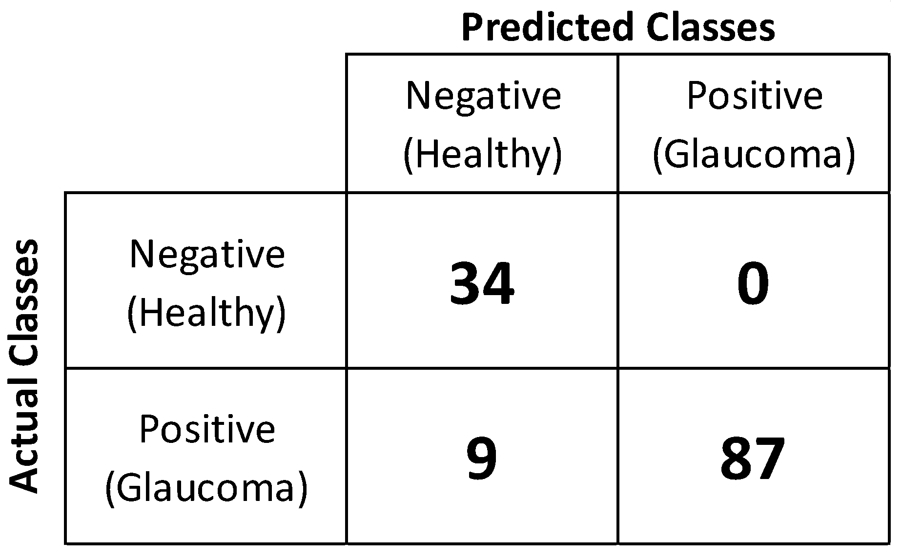
In this study, we performed nine deep learning (DL) pre-trained models for evaluating our processed data. The nine pre-trained models were AlexNet [55], GoogleNet [56], Inception V3 [57], XceptionNet [58], ResNet-50 [59], InceptionResNet [60], MobileNet [61], NasNet [62], and DenseNet [63]. The configuration of each network is described in

Table 3. Configuration and properties of each deep learning pre-trained model.

Network [Ref.]	Depth	Size (MB)	Parameters	Input Size
AlexNet [55]	8	227	58,266,306	227 × 227
GoogleNet [56]	22	27	1,252,072	224 × 224
Inception V3 [57]	48	89	23,855,837	299 × 299
XceptionNet [58]	71	85	20,865,578	299 × 299
ResNet-50 [59]	107	98	23,591,810	224 × 224
InceptionResNet [60]	164	209	26,530,290	299 × 299
MobileNet [61]	53	13	4,256,893	224 × 224
NasNet [62]	*	360	5,329,777	331 × 331
DenseNet [63]	201	77	7,039,554	224 × 224

. The input images for all those networks are RGB images.

3. Results

In the first step of our experiment, we removed the blood vessel and optic disc by applying a heuristic method of a blood vessel and optic disc segmentation. The result of this process is illustrated in Figure 12. Images in Figure 12 illustrate the process of pre-processing steps. Figure 12 illustrates the results of each process, including those of the localization process, segmentation of OD, and segmentation of blood vessels. As illustrated in Figure 12, our localization method is suitable to recognize the location of the OD candidate. The result of localization is depicted with a red rectangle in Figure 12. For the overall localization process, our proposed method successfully achieved an accuracy of 100%, which means that our proposed method can precisely recognize all OD. After finding the location of OD, we conducted the OD segmentation. The result of this process can be seen in the step of OD segmentation shown in Figure 12. This result illustrates that the segmented optic disc seems close to the OD in the original images. Since the ORIGA-light dataset also provided an optic disc ground truth, then we evaluated our segmentation method and achieved an accuracy of 93.61%.

According to the optic disc segmentation result that appeared in Figure 12 and achievement accuracy, we concluded that our proposed OD segmentation method was powerful enough to find and segment the optic disc area. After the OD segmentation was accomplished, the process was continued with blood vessel segmentation. In the next step, we conducted a blood vessel segmentation process by using a heuristic method, as described in Section 2. This process was started by multiplying the segmented OD with the original image, then, it was followed by extracting the green channel extraction. As our goal was that RNFL should become the major object to be analyzed, the green channel was chosen, because RNFL seemed clearer than RGB. The result of the blood vessel segmentation can be seen in the step of blood vessel segmentation shown in Figure 12. Since ORIGA-light did not provide the ground truth of blood vessels, we evaluated our segmentation process by analyzing the result visually. However, as depicted in Figure 12, almost the entire blood vessel area is successfully segmented. The last picture in Figure 12 illustrates the final result of the pre-processing step, which was the fundus image without the optic disc and blood vessel. This picture then became the input image of the deep learning process.

In the next step, we performed a data augmentation process to alleviate the data imbalance problem. Before that, the dataset was then separated into training and testing parts, with a proportion of 80% (520) of data set up as training data and 20% (130) of data set up as testing data. To reach this goal, we applied the SMOTE filter function to the training data and achieved balanced training data of 1460 images. We utilized this training data on nine deep learning architectures using a transfer learning pre-trained model, as outlined in Table 3. On each of the training processes, the images were resized to satisfy the pixel dimension required by the corresponding pre-trained model. The results of our experiment are presented in

Table 4. Comparison results to a previous study that had similar scenarios.

Network [Ref.]	Input Size	Accuracy (%)
		Sreng et al. (2020) [64]		Our Proposed Model (2022)
		Pre-Trained Model	CNN+SVM
AlexNet [55]	227 × 227	68.42	76.41	92.61
GoogleNet [56]	224 × 224	71.79	74.87	87.95
Inception V3 [57]	299 × 299	75.38	78.97	75.57
XceptionNet [58]	299 × 299	77.44	75.9	71.76
ResNet-50 [59]	224 × 224	75.9	75.38	84.93
InceptionResNet [60]	299 × 299	80	78.46	74.05
MobileNet [61]	224 × 224	80.51	74.36	75.57
NasNet [62]	331 × 331	73.85	74.87	78.63
DenseNet [63]	224 × 224	77.44	78.46	92.88

. In Table 4, we also presented the result of the pre-trained model tested in the testing data of the ORIGA-Light dataset without any pre-treatment processes. In addition, we compared our work with a previous study that had similar experiment scenarios.

Table 4 demonstrates the results of our experiments compared to two different approaches. The pre-trained model conducted by [64] was carried out by utilizing the original CNN pre-trained model without any additional treatment. They used the original cropped optic disc of the ORIGA-Light dataset as input images. According to Table 4, MobileNet performed the best in the ORIGA-Light dataset, with an accuracy of 80%, followed by InceptionResNet, with an accuracy of 90%, and XceptionNet and DenseNet, with similar accuracies of 77.44% each. Whilst, the CNN+SVM proposed by Sreng et al. [64] achieved an accuracy of less than 80% in all deep learning architecture. The highest performance of this method was carried out by Inception V3, with an accuracy of 78.97%, followed by InceptionResNet dan DenseNet, with similar accuracies of 78.46% each.

Similar to the previous study, this method used cropped optic discs as input images in their deep learning model. Those results show that their proposed method was good enough in the ORIGA-Light dataset. Offering another solution, we proposed a different way to analyze glaucoma disease. We used the characteristic of RNFL as the major object to recognize the progression of glaucoma disease. In our experiments, almost all deep learning architectures achieved good enough performance. The highest accuracy was carried out by DenseNet, with an accuracy of 92.88%, followed by AlexNet, with an accuracy of 92.61%, and GoogleNet, with an accuracy of 87.95%. This result successfully improved by more than 15% from the two previous research works proposed by [64]. According to the results presented in Table 4, we might conclude that our proposed method was suitable enough to recognize glaucoma in the ORIGA-Light dataset with the highest accuracy, as compared to other models and previous studies techniques, with a more than 15% accuracy improvement.

The confusion matrix shown in Figure 13 was provided to add more detailed information about the model performance. The confusion matrix depicted in Figure 13 was obtained by performing DenseNet. This result indicated that utilizing RNFL became a proper and effective solution to analyze the progression of glaucoma disease. In addition, Figure 14 is an example of the classification results predicted by DenseNet, using the image data preprocessed by our proposed approach. Figure 14a,b show the glaucomatous and normal eyes, respectively.

4. Discussions

The intelligent glaucoma detection system played the role of an essential tool used to monitor the progression of glaucoma disease more objectively and reliably. This intelligent system was able to assist medical personnel in recognizing glaucoma symptoms faster and more cheaply. Currently, several research undertakings have been performed, aiming to aid in the development of an automated glaucoma detection system. Almost all of those research works used optic discs and optic cups as input data to detect the presence of glaucoma. However, utilizing the optic disc and optic cup as a major object to diagnose glaucoma was extremely risky due to the differences between the optic disc and optic cup of each patient. This condition often leads to misinterpretation.

The ORIGA-Light dataset was one of the most popular glaucoma datasets that was often used by several researchers. The ORIGA-Light dataset had a variety of data that was quite complex. It was proven by previous results, as illustrated in Table 4, though it could not easily achieve an accuracy of more than 90%. Regarding that problem, we offered an alternative way of evaluating glaucoma disease. We considered analyzing RNFL instead of using an optic disc and optic cup, due to their uncertain standard of size.

We compared our proposed method with previous works that used the same dataset for glaucoma classification purposes.

Table 5. Comparison results with findings from earlier works.

Reference	Accuracy (%)	AUC (%)	Notes
[64]	88.86	83.59	Experiment 1: using CNN pre-trained model
[64]	85.26	80	Experiment 2: using CNN+SVM
[65]	-	86.8	Experiment 1: using a random training technique
[65]	-	87.4	Experiment 2: using cross-validation
[66]	-	83.1	-
[67]	-	83.8	-
[68]	-	83.8	-
[69]	-	82.3	-
[32]	-	85.1	-
[40]	-	84.83	-
[41]	91.2	-	-
Our proposed method (2022)	92.88	89.34	Using DenseNet

illustrates the comparison result of our proposed method to other different ways of glaucoma classification using the ORIGA-Light dataset. According to Table 5, it can be recognized that our proposed solution successfully outperformed several previous studies, with an accuracy of 92.88% and an AUC of 89.34%.

As demonstrated in Table 4 and Table 5, we can conclude that our proposed solution successfully outperformed the previous research works. Hence, it can be inferred that analyzing RNFL was more suitable for recognizing the presence of glaucoma than using an optic disc and optic cup, particularly given the complex dataset. This result also proves the medical theory [24] that measuring the thickness of RNFL is an objective and reliable way to monitor the progression of glaucoma disease. Therefore, it is expected that our proposed model could help improve eye disease diagnosis and assessment.

5. Practical Application

Artificial intelligence (AI) and machine learning (ML)-based diagnostics have been widely utilized by researchers and practitioners to detect risks and facilitate decision-making in a range of contexts, from the prediction of chronic diseases like cancer [70,71] to psychological disorders [72]. Therefore, this ML-based deep learning model yield in this experiment can be further implemented in web/mobile-based applications for practical usage and gives maximum benefits of early glaucoma detection to the worldwide community. Hence, the further objective of this work is to design and implement an early glaucoma detection platform. This platform then can be implemented as Software as a Service (SaaS) to facilitate medical teams’ decision-making in glaucoma screening.

In this research, we demonstrated the practicability of our developed model using the TensorFlow framework implemented using Python programming language. Python has a feature which allows the trained model to be saved on the specified so-called HDF5 filesystem. HDF5 (Hierarchical Data Format version 5) is an open-source file format that supports large, complex, and heterogeneous data, which is perfectly suited to save the distributed representation of the DL model and its weights. Since Python seamlessly supports HDF5, we then used Python-based architecture as the main ingredient for the glaucoma detection platform and provided API (Application Programming Interface) services for this purpose. Figure 14 illustrates the workflow and architecture of the proposed system design. In the architecture depicted in Figure 15, an application can be accessed by the user (the medical team) either through their personal computer (PC) and a web browser, or through their mobile device and an application that is connected to the fundus camera.

The proposed architecture required a fundus camera as the input device. A fundus camera is a specified device used for fundus photography. The back of the eye, also called the fundus, is the subject of photography in the field of fundus photography. In fundus photography, the usage of specialized fundus cameras that consist of a complex microscope attached to a camera with a flash capability is required [73]. The central and peripheral retina, optic disc, and macula are the primary components that can be seen in a fundus photograph. Other structures, such as the choroid, may also be visible. Photography of the fundus can be done using colored filters or with specific dyes like fluorescein and indocyanine green [74]. Currently, many types of fundus cameras with various specifications are widely available on the market. Figure 16 shows a picture of a fundus camera that is typically used in a healthcare facility.

The fundus camera serves as an input device that scans the eyes in order to provide an accurate image of the eye. That image is then transmitted together with the feature data. After that, the input feature data are sent to a web server, where our proposed model is utilized to determine whether or not the subjects in question have glaucoma. The user is then supplied with the result of the diagnosis using the interface for the prediction output. Figure 17, below, shows the design of a mobile application prototype in which users can interact with the early glaucoma diagnostic platform. Users can take an image of an eye for diagnostic using the application connected to the fundus camera, as shown in Figure 17a, then the user can submit the image to the proposed cloud platform and have information about the diagnostic result sent back to the mobile application, as shown in Figure 17b.

Our proposed model may not be used for general subjects because it was only trained on a particular dataset. Additionally, due to the constraints of the dataset used in our research, we did not apply the model to clinical trials with real patients. We could do clinical studies by working with doctors or university hospitals once another group of demographic subjects (for instance, in Indonesia and Republic of Korea) is gathered, but that is currently outside the scope of our current study.

6. Conclusions

Our research work presented the development of intelligent tools for monitoring the progression of glaucoma disease as more objective and reliable. Our proposed solution is comprised of two major processes; the pre-treatment process and the classification process. In the pre-treatment process, we removed unnecessary parts, such as the optic disc and blood vessels. Those two parts are considered for removal since they might be obstacles in the analysis process. For the classification stages, we used nine deep-learning architectures. We evaluated our proposed method in the ORIGA dataset and achieved an accuracy of 93.61% in the segmentation process, and the highest accuracy of 92.88% with an AUC of 89.34% in the classification process. This result is improved by more than 15% from the previous research work. Finally, it is expected that having an improved glaucoma detection model could help improve eye disease diagnosis and assessment.

Despite the promising nature of our findings, future research will still be necessary to develop a better method. One of the limitations of our experiment was that we restricted our experiment only to the ORIGA-Light dataset, and a different performance may be provided by another dataset. Additionally, we did not consider the computational time performance of our method; therefore, considering this factor would be beneficial for improving the diagnosis time, as well as the performance of our current findings.

References

1. Diaz-Pinto, A.; Colomer, A.; Naranjo, V.; Morales, S.; Xu, Y.; Frangi, A.F. Retinal Image Synthesis and Semi-Supervised Learning for Glaucoma Assessment. IEEE Trans. Med. Imaging 2019, 38, 2211–2218. [Google Scholar] [CrossRef] [PubMed]
2. Stella Mary, M.C.V.; Rajsingh, E.B.; Naik, G.R. Retinal Fundus Image Analysis for Diagnosis of Glaucoma: A Comprehensive Survey. IEEE Access 2016, 4, 4327–4354. [Google Scholar] [CrossRef]
3. Yu, S.; Xiao, D.; Frost, S.; Kanagasingam, Y. Robust Optic Disc and Cup Segmentation with Deep Learning for Glaucoma Detection. Comput. Med. Imaging Graph. 2019, 74, 61–71. [Google Scholar] [CrossRef] [PubMed]
4. Claro, M.; Veras, R.; Santana, A.; Araújo, F.; Silva, R.; Almeida, J.; Leite, D. An Hybrid Feature Space from Texture Information and Transfer Learning for Glaucoma Classification. J. Vis. Commun. Image Represent. 2019, 64, 102597. [Google Scholar] [CrossRef]
5. Mvoulana, A.; Kachouri, R.; Akil, M. Fully Automated Method for Glaucoma Screening Using Robust Optic Nerve Head Detection and Unsupervised Segmentation Based Cup-to-Disc Ratio Computation in Retinal Fundus Images. Comput. Med. Imaging Graph. 2019, 77, 101643. [Google Scholar] [CrossRef]
6. Odstrčilík, J.; Kolář, R.; Harabiš, V.; Gazárek, J. Jan Retinal Nerve Fiber Layer Analysis via Markov Random Fields Texture Modelling. In Proceedings of the 2010 18th European Signal Processing Conference, Aalborg, Denmark, 23–27 August 2010; pp. 1650–1654. [Google Scholar]
7. Lu, S.-H.; Lee, K.Y.; Chong, J.I.T.; Lam, A.K.C.; Lai, J.S.M.; Lam, D.C.C. Comparison of Ocular Biomechanical Machine Learning Classifiers for Glaucoma Diagnosis. In Proceedings of the 2018 IEEE International Conference on Bioinformatics and Biomedicine (BIBM), Madrid, Spain, 3–6 December 2018; IEEE: Madrid, Spain, 2018; pp. 2539–2543. [Google Scholar]
8. Thangaraj, V.; Natarajan, V. Glaucoma Diagnosis Using Support Vector Machine. In Proceedings of the 2017 International Conference on Intelligent Computing and Control Systems (ICICCS), Madurai, India, 15–16 June 2017; pp. 394–399. [Google Scholar]
9. Shalini, S.; Srinivasan, N. WITHDRAWN: Retinal Image Classification by Glaucoma Based on ANFIS Classifier. Mater. Today Proc. 2021, S2214785320407746. [Google Scholar] [CrossRef]
10. Dixit, A.; Yohannan, J.; Boland, M.V. Assessing Glaucoma Progression Using Machine Learning Trained on Longitudinal Visual Field and Clinical Data. Ophthalmology 2021, 128, 1016–1026. [Google Scholar] [CrossRef]
11. Wang, P.; Shen, J.; Chang, R.; Moloney, M.; Torres, M.; Burkemper, B.; Jiang, X.; Rodger, D.; Varma, R.; Richter, G.M. Machine Learning Models for Diagnosing Glaucoma from Retinal Nerve Fiber Layer Thickness Maps. Ophthalmol. Glaucoma 2019, 2, 422–428. [Google Scholar] [CrossRef]
12. Thakur, N.; Juneja, M. Classification of Glaucoma Using Hybrid Features with Machine Learning Approaches. Biomed. Signal Process. Control 2020, 62, 102137. [Google Scholar] [CrossRef]
13. Bhat, S.A.; Huang, N.-F.; Hussain, I.; Bibi, F.; Sajjad, U.; Sultan, M.; Alsubaie, A.S.; Mahmoud, K.H. On the Classification of a Greenhouse Environment for a Rose Crop Based on AI-Based Surrogate Models. Sustainability 2021, 13, 12166. [Google Scholar] [CrossRef]
14. Yan, H.; Sergin, N.D.; Brenneman, W.A.; Lange, S.J.; Ba, S. Deep Multistage Multi-Task Learning for Quality Prediction of Multistage Manufacturing Systems. J. Qual. Technol. 2021, 53, 526–544. [Google Scholar] [CrossRef]
15. Almeida, A.; Azkune, G. Predicting Human Behaviour with Recurrent Neural Networks. Appl. Sci. 2018, 8, 305. [Google Scholar] [CrossRef] [Green Version]
16. Raghavendra, U.; Fujita, H.; Bhandary, S.V.; Gudigar, A.; Tan, J.H.; Acharya, U.R. Deep Convolution Neural Network for Accurate Diagnosis of Glaucoma Using Digital Fundus Images. Inf. Sci. 2018, 441, 41–49. [Google Scholar] [CrossRef]
17. Vinícius dos Santos Ferreira, M.; Oseas de Carvalho Filho, A.; Dalília de Sousa, A.; Corrêa Silva, A.; Gattass, M. Convolutional Neural Network and Texture Descriptor-Based Automatic Detection and Diagnosis of Glaucoma. Expert Syst. Appl. 2018, 110, 250–263. [Google Scholar] [CrossRef]
18. Al-Bander, B.; Al-Nuaimy, W.; Al-Taee, M.A.; Zheng, Y. Automated Glaucoma Diagnosis Using Deep Learning Approach. In Proceedings of the 2017 14th International Multi-Conference on Systems, Signals & Devices (SSD), Marrakech, Morocco, 28–31 March 2017; pp. 207–210. [Google Scholar]
19. Norouzifard, M.; Nemati, A.; GholamHosseini, H.; Klette, R.; Nouri-Mahdavi, K.; Yousefi, S. Automated Glaucoma Diagnosis Using Deep and Transfer Learning: Proposal of a System for Clinical Testing. In Proceedings of the 2018 International Conference on Image and Vision Computing New Zealand (IVCNZ), Auckland, New Zealand, 19–21 November 2018; pp. 1–6. [Google Scholar]
20. Phasuk, S.; Poopresert, P.; Yaemsuk, A.; Suvannachart, P.; Itthipanichpong, R.; Chansangpetch, S.; Manassakorn, A.; Tantisevi, V.; Rojanapongpun, P.; Tantibundhit, C. Automated Glaucoma Screening from Retinal Fundus Image Using Deep Learning. In Proceedings of the 2019 41st Annual International Conference of the IEEE Engineering in Medicine and Biology Society (EMBC), Berlin, Germany, 23–27 July 2019; pp. 904–907. [Google Scholar]
21. Zheng, X.; Wang, M.; Ordieres-Meré, J. Comparison of Data Preprocessing Approaches for Applying Deep Learning to Human Activity Recognition in the Context of Industry 4.0. Sensors 2018, 18, 2146. [Google Scholar] [CrossRef] [Green Version]
22. Al-Tam, R.M.; Al-Hejri, A.M.; Narangale, S.M.; Samee, N.A.; Mahmoud, N.F.; Al-masni, M.A.; Al-antari, M.A. A Hybrid Workflow of Residual Convolutional Transformer Encoder for Breast Cancer Classification Using Digital X-Ray Mammograms. Biomedicines 2022, 10, 2971. [Google Scholar] [CrossRef]
23. Saleh, O.; Nozaki, K.; Matsumura, M.; Yanaka, W.; Miura, H.; Fueki, K. Texture-Based Neural Network Model for Biometric Dental Applications. JPM 2022, 12, 1954. [Google Scholar] [CrossRef]
24. RNFL Analysis in the Diagnosis of Glaucoma. Available online: https://glaucomatoday.com/articles/2016-may-june/rnfl-analysis-in-the-diagnosis-of-glaucoma (accessed on 12 October 2022).
25. Zhang, Z.; Yin, F.S.; Liu, J.; Wong, W.K.; Tan, N.M.; Lee, B.H.; Cheng, J.; Wong, T.Y. ORIGA-light: An Online Retinal Fundus Image Database for Glaucoma Analysis and Research. In Proceedings of the 2010 Annual International Conference of the IEEE Engineering in Medicine and Biology, Buenos Aires, Argentina, 31 August–4 September 2010; pp. 3065–3068. [Google Scholar]
26. Wang, L.; Gu, J.; Chen, Y.; Liang, Y.; Zhang, W.; Pu, J.; Chen, H. Automated Segmentation of the Optic Disc from Fundus Images Using an Asymmetric Deep Learning Network. Pattern Recognit. 2021, 112, 107810. [Google Scholar] [CrossRef]
27. Liu, S.; Hong, J.; Lu, X.; Jia, X.; Lin, Z.; Zhou, Y.; Liu, Y.; Zhang, H. Joint Optic Disc and Cup Segmentation Using Semi-Supervised Conditional GANs. Comput. Biol. Med. 2019, 115, 103485. [Google Scholar] [CrossRef]
28. Yin, P.; Xu, Y.; Zhu, J.; Liu, J.; Yi, C.; Huang, H.; Wu, Q. Deep Level Set Learning for Optic Disc and Cup Segmentation. Neurocomputing 2021, 464, 330–341. [Google Scholar] [CrossRef]
29. Liu, Q.; Hong, X.; Li, S.; Chen, Z.; Zhao, G.; Zou, B. A Spatial-Aware Joint Optic Disc and Cup Segmentation Method. Neurocomputing 2019, 359, 285–297. [Google Scholar] [CrossRef]
30. Tulsani, A.; Kumar, P.; Pathan, S. Automated Segmentation of Optic Disc and Optic Cup for Glaucoma Assessment Using Improved UNET++ Architecture. Biocybern. Biomed. Eng. 2021, 41, 819–832. [Google Scholar] [CrossRef]
31. Sun, X.; Xu, Y.; Zhao, W.; You, T.; Liu, J. Optic Disc Segmentation from Retinal Fundus Images via Deep Object Detection Networks. In Proceedings of the 2018 40th Annual International Conference of the IEEE Engineering in Medicine and Biology Society (EMBC), Honolulu, HI, USA, 17–21 July 2018; pp. 5954–5957. [Google Scholar]
32. Fu, H.; Cheng, J.; Xu, Y.; Wong, D.W.K.; Liu, J.; Cao, X. Joint Optic Disc and Cup Segmentation Based on Multi-Label Deep Network and Polar Transformation. IEEE Trans. Med. Imaging 2018, 37, 1597–1605. [Google Scholar] [CrossRef] [PubMed] [Green Version]
33. Niu, D.; Xu, P.; Wan, C.; Cheng, J.; Liu, J. Automatic Localization of Optic Disc Based on Deep Learning in Fundus Images. In Proceedings of the 2017 IEEE 2nd International Conference on Signal and Image Processing (ICSIP), Singapore, 4–6 August 2017; pp. 208–212. [Google Scholar]
34. Liu, Q.; Zou, B.; Zhao, Y.; Liang, Y. A Deep Gradient Boosting Network for Optic Disc and Cup Segmentation. In Proceedings of the ICASSP 2020—2020 IEEE International Conference on Acoustics, Speech and Signal Processing (ICASSP), Barcelona, Spain, 4–8 May 2020; pp. 971–975. [Google Scholar]
35. Liao, C.-L.; Chou, C.-A.; Chen, C.-Y.; Wang, Y.-K. Retinal Fundus Image Segmentation Based on Channel-Attention Guided Network. In Proceedings of the 2022 5th International Conference on Pattern Recognition and Artificial Intelligence (PRAI), Chengdu, China, 19–21 August 2022; pp. 1055–1059. [Google Scholar]
36. Cheng, P.; Lyu, J.; Huang, Y.; Tang, X. Probability Distribution Guided Optic Disc and Cup Segmentation from Fundus Images. In Proceedings of the 2020 42nd Annual International Conference of the IEEE Engineering in Medicine & Biology Society (EMBC), Montreal, QC, Canada, 20–24 July 2020; pp. 1976–1979. [Google Scholar]
37. Singh, L.K.; Khanna, M.; Thawkar, S.; Singh, R. Collaboration of Features Optimization Techniques for the Effective Diagnosis of Glaucoma in Retinal Fundus Images. Adv. Eng. Softw. 2022, 173, 103283. [Google Scholar] [CrossRef]
38. Balasubramanian, K.; Ananthamoorthy, N.P. Correlation-Based Feature Selection Using Bio-Inspired Algorithms and Optimized KELM Classifier for Glaucoma Diagnosis. Appl. Soft Comput. 2022, 128, 109432. [Google Scholar] [CrossRef]
39. Balasubramanian, K.; Ramya, K.; Gayathri Devi, K. Improved Swarm Optimization of Deep Features for Glaucoma Classification Using SEGSO and VGGNet. Biomed. Signal Process. Control 2022, 77, 103845. [Google Scholar] [CrossRef]
40. Li, A.; Wang, Y.; Cheng, J.; Liu, J. Combining Multiple Deep Features for Glaucoma Classification. In Proceedings of the 2018 IEEE International Conference on Acoustics, Speech and Signal Processing (ICASSP), Calgary, AB, USA, 15–20 April 2018; pp. 985–989. [Google Scholar]
41. Elakkiya, B.; Saraniya, O. A Comparative Analysis of Pretrained and Transfer-Learning Model for Automatic Diagnosis of Glaucoma. In Proceedings of the 2019 11th International Conference on Advanced Computing (ICoAC), Chennai, India, 18–20 December 2019; pp. 167–172. [Google Scholar]
42. Fan, R.; Alipour, K.; Bowd, C.; Christopher, M.; Brye, N.; Proudfoot, J.A.; Goldbaum, M.H.; Belghith, A.; Girkin, C.A.; Fazio, M.A.; et al. Detecting Glaucoma from Fundus Photographs Using Deep Learning without Convolutions: Transformer for Improved Generalization. Ophthalmol. Sci. 2022, 3, 100233. [Google Scholar] [CrossRef]
43. Patel, A.S.; Singh, V. Glaucoma Detection Using Mask Region-Based Convolutional Neural Networks. In Proceedings of the 2021 5th International Conference on Electronics, Communication and Aerospace Technology (ICECA), Coimbatore, India, 2–4 December 2021; pp. 1642–1647. [Google Scholar]
44. Li, S.; Li, Z.; Guo, L.; Bian, G.-B. Glaucoma Detection: Joint Segmentation and Classification Framework via Deep Ensemble Network. In Proceedings of the 2020 5th International Conference on Advanced Robotics and Mechatronics (ICARM), Shenzhen, China, 18–21 December 2020; pp. 678–685. [Google Scholar]
45. Saxena, A.; Vyas, A.; Parashar, L.; Singh, U. A Glaucoma Detection Using Convolutional Neural Network. In Proceedings of the 2020 International Conference on Electronics and Sustainable Communication Systems (ICESC), Coimbatore, India, 2–4 July 2020; pp. 815–820. [Google Scholar]
46. Al-Muswi, W.A.K.; Al-Saadi, E.H. Extraction of The Neural Edge and Its Properties for The Retina Infected with Glaucoma. In Proceedings of the 2021 International Conference on Advance of Sustainable Engineering and Its Application (ICASEA), Wasit, Iraq, 27–28 October 2021; pp. 89–93. [Google Scholar]
47. Zhao, R.; Chen, X.; Liu, X.; Chen, Z.; Guo, F.; Li, S. Direct Cup-to-Disc Ratio Estimation for Glaucoma Screening via Semi-Supervised Learning. IEEE J. Biomed. Health Inform. 2020, 24, 1104–1113. [Google Scholar] [CrossRef]
48. Deperlioglu, O.; Kose, U.; Gupta, D.; Khanna, A.; Giampaolo, F.; Fortino, G. Explainable Framework for Glaucoma Diagnosis by Image Processing and Convolutional Neural Network Synergy: Analysis with Doctor Evaluation. Future Gener. Comput. Syst. 2022, 129, 152–169. [Google Scholar] [CrossRef]
49. Liao, W.; Zou, B.; Zhao, R.; Chen, Y.; He, Z.; Zhou, M. Clinical Interpretable Deep Learning Model for Glaucoma Diagnosis. IEEE J. Biomed. Health Inform. 2020, 24, 1405–1412. [Google Scholar] [CrossRef]
50. Chan, T.F.; Vese, L.A. Active Contours without Edges. IEEE Trans. Image Process. 2001, 10, 266–277. [Google Scholar] [CrossRef] [Green Version]
51. Reza, A.M. Realization of the Contrast Limited Adaptive Histogram Equalization (CLAHE) for Real-Time Image Enhancement. J. VLSI Signal Process. -Syst. Signal Image Video Technol. 2004, 38, 35–44. [Google Scholar] [CrossRef]
52. Otsu, N. A Threshold Selection Method from Gray-Level Histograms. IEEE Trans. Syst. Man Cybern. 1979, 9, 62–66. [Google Scholar] [CrossRef] [Green Version]
53. Chawla, N.V. Data Mining for Imbalanced Datasets: An Overview. In Data Mining and Knowledge Discovery Handbook; Maimon, O., Rokach, L., Eds.; Springer: New York, NY, USA, 2005; pp. 853–867. ISBN 978-0-38724-435-8. [Google Scholar]
54. Douzas, G.; Bacao, F.; Last, F. Improving Imbalanced Learning through a Heuristic Oversampling Method Based on K-Means and SMOTE. Inf. Sci. 2018, 465, 1–20. [Google Scholar] [CrossRef] [Green Version]
55. Krizhevsky, A.; Sutskever, I.; Hinton, G.E. ImageNet Classification with Deep Convolutional Neural Networks. Commun. ACM 2017, 60, 84–90. [Google Scholar] [CrossRef] [Green Version]
56. Szegedy, C.; Liu, W.; Jia, Y.; Sermanet, P.; Reed, S.; Anguelov, D.; Erhan, D.; Vanhoucke, V.; Rabinovich, A. Going Deeper with Convolutions. In Proceedings of the 2015 IEEE Conference on Computer Vision and Pattern Recognition (CVPR), Boston, MA, USA, 7–12 June 2015; pp. 1–9. [Google Scholar]
57. Szegedy, C.; Vanhoucke, V.; Ioffe, S.; Shlens, J.; Wojna, Z. Rethinking the Inception Architecture for Computer Vision. In Proceedings of the 2016 IEEE Conference on Computer Vision and Pattern Recognition (CVPR), Las Vegas, NV, USA, 27–30 June 2016; pp. 2818–2826. [Google Scholar]
58. Chollet, F. Xception: Deep Learning with Depthwise Separable Convolutions. In Proceedings of the 2017 IEEE Conference on Computer Vision and Pattern Recognition (CVPR), Honolulu, HI, USA, 21–26 July 2017; pp. 1800–1807. [Google Scholar]
59. He, K.; Zhang, X.; Ren, S.; Sun, J. Deep Residual Learning for Image Recognition. In Proceedings of the 2016 IEEE Conference on Computer Vision and Pattern Recognition (CVPR), Las Vegas, NV, USA, 27–30 June 2016; pp. 770–778. [Google Scholar]
60. Szegedy, C.; Ioffe, S.; Vanhoucke, V.; Alemi, A. Inception-v4, Inception-ResNet and the Impact of Residual Connections on Learning. Assoc. Adv. Artif. Intell. 2017, 31. [Google Scholar] [CrossRef]
61. Howard, A.G.; Zhu, M.; Chen, B.; Kalenichenko, D.; Wang, W.; Weyand, T.; Andreetto, M.; Adam, H. MobileNets: Efficient Convolutional Neural Networks for Mobile Vision Applications. arXiv 2017, arXiv:1704.04861. [Google Scholar]
62. Zoph, B.; Vasudevan, V.; Shlens, J.; Le, Q.V. Learning Transferable Architectures for Scalable Image Recognition. In Proceedings of the 2018 IEEE/CVF Conference on Computer Vision and Pattern Recognition, Salt Lake City, UT, USA, 18–23 June 2018; pp. 8697–8710. [Google Scholar]
63. Huang, G.; Liu, Z.; Van Der Maaten, L.; Weinberger, K.Q. Densely Connected Convolutional Networks. In Proceedings of the 2017 IEEE Conference on Computer Vision and Pattern Recognition (CVPR), Honolulu, HI, USA, 21–26 July 2017; pp. 2261–2269. [Google Scholar]
64. Sreng, S.; Maneerat, N.; Hamamoto, K.; Win, K.Y. Deep Learning for Optic Disc Segmentation and Glaucoma Diagnosis on Retinal Images. Appl. Sci. 2020, 10, 4916. [Google Scholar] [CrossRef]
65. Bajwa, M.N.; Malik, M.I.; Siddiqui, S.A.; Dengel, A.; Shafait, F.; Neumeier, W.; Ahmed, S. Correction to: Two-Stage Framework for Optic Disc Localization and Glaucoma Classification in Retinal Fundus Images Using Deep Learning. BMC Med. Inf. Decis. Mak. 2019, 19, 153. [Google Scholar] [CrossRef] [Green Version]
66. Chen, X.; Xu, Y.; Kee Wong, D.W.; Wong, T.Y.; Liu, J. Glaucoma Detection Based on Deep Convolutional Neural Network. In Proceedings of the 2015 37th Annual International Conference of the IEEE Engineering in Medicine and Biology Society (EMBC), Milan, Italy, 25–29 August 2015; pp. 715–718. [Google Scholar]
67. Chen, X.; Xu, Y.; Yan, S.; Wong, D.W.K.; Wong, T.Y.; Liu, J. Automatic Feature Learning for Glaucoma Detection Based on Deep Learning. In Medical Image Computing and Computer-Assisted Intervention–MICCAI 2015; Navab, N., Hornegger, J., Wells, W.M., Frangi, A.F., Eds.; Lecture Notes in Computer Science; Springer International Publishing: Cham, Switzerland, 2015; Volume 9351, pp. 669–677. ISBN 978-3-31924-573-7. [Google Scholar]
68. Xu, Y.; Lin, S.; Wong, D.W.K.; Liu, J.; Xu, D. Efficient Reconstruction-Based Optic Cup Localization for Glaucoma Screening. In Advanced Information Systems Engineering; Salinesi, C., Norrie, M.C., Pastor, Ó., Eds.; Lecture Notes in Computer Science; Springer: Berlin, Heidelberg, 2013; Volume 7908, pp. 445–452. ISBN 978-3-64238-708-1. [Google Scholar]
69. Li, A.; Cheng, J.; Wong, D.W.K.; Liu, J. Integrating Holistic and Local Deep Features for Glaucoma Classification. In Proceedings of the 2016 38th Annual International Conference of the IEEE Engineering in Medicine and Biology Society (EMBC), Orlando, FL, USA, 16–20 August 2016; pp. 1328–1331. [Google Scholar]
70. Al-antari, M.A.; Al-masni, M.A.; Choi, M.-T.; Han, S.-M.; Kim, T.-S. A Fully Integrated Computer-Aided Diagnosis System for Digital X-Ray Mammograms via Deep Learning Detection, Segmentation, and Classification. Int. J. Med. Inform. 2018, 117, 44–54. [Google Scholar] [CrossRef]
71. Alfian, G.; Syafrudin, M.; Fahrurrozi, I.; Fitriyani, N.L.; Atmaji, F.T.D.; Widodo, T.; Bahiyah, N.; Benes, F.; Rhee, J. Predicting Breast Cancer from Risk Factors Using SVM and Extra-Trees-Based Feature Selection Method. Computers 2022, 11, 136. [Google Scholar] [CrossRef]
72. Lipschitz, J.; Miller, C.J.; Hogan, T.P.; Burdick, K.E.; Lippin-Foster, R.; Simon, S.R.; Burgess, J. Adoption of Mobile Apps for Depression and Anxiety: Cross-Sectional Survey Study on Patient Interest and Barriers to Engagement. JMIR Ment. Health 2019, 6, e11334. [Google Scholar] [CrossRef] [PubMed] [Green Version]
73. Panwar, N.; Huang, P.; Lee, J.; Keane, P.A.; Chuan, T.S.; Richhariya, A.; Teoh, S.; Lim, T.H.; Agrawal, R. Fundus Photography in the 21st Century—A Review of Recent Technological Advances and Their Implications for Worldwide Healthcare. Telemed. E-Health 2016, 22, 198–208. [Google Scholar] [CrossRef] [PubMed]
74. Bernardes, R.; Serranho, P.; Lobo, C. Digital Ocular Fundus Imaging: A Review. Ophthalmologica 2011, 226, 161–181. [Google Scholar] [CrossRef]
75. File:Retinal camera.jpg-Wikimedia Commons. Available online: https://commons.wikimedia.org/wiki/File:Retinal_camera.jpg (accessed on 1 December 2022).
Figure 1. An example of (a) OD (marked by a white circle) and OC (marked by a black circle) indicates a healthy optic nerve, (b) OD (marked by a white circle) and OC (marked by a black circle) indicates a glaucomatous optic nerve and (c) glaucoma location [3,6].
Applsci 13 00037 g001
Figure 2. Flowchart of our proposed method.
Applsci 13 00037 g002
Figure 3. The scheme of preprocessing process.
Applsci 13 00037 g003
Figure 4. The algorithm of optic disc localization.
Applsci 13 00037 g004
Figure 5. The fringe (a) is shown by the white arrows. To eliminate the fringe, a frame (b) is added on the side of the image.
Applsci 13 00037 g005
Figure 6. The differences appeared in (a) red channel image, (b) green channel image, and (c) blue channel image.
Applsci 13 00037 g006aApplsci 13 00037 g006b
Figure 7. The illustration of (a) the RoI marked by a red rectangle with size 702 by 702 pixels and (b) the cropped RoI from the rectangle.
Applsci 13 00037 g007
Figure 8. The flow process of pretreatment.
Applsci 13 00037 g008
Figure 9. Red channel extraction. RoI before the extraction (a) and the RoI after the extraction leaving only a red channel on the image (b).
Applsci 13 00037 g009
Figure 10. Illustration of (a) the segmented optic disc is presented as a binary image. The white part is the optic disc while the black is the background and (b) the part on the side of the image is the artifacts included in the segmentation process yielding an incorrect representation of the optic disc.
Applsci 13 00037 g010
Figure 11. An illustration of the SMOTE filter function with k = 4.
Applsci 13 00037 g011
Figure 12. Result of a pre-processing step including localization step, OD segmentation, and blood vessel segmentation.
Applsci 13 00037 g012
Figure 13. Confusion matrix of DenseNet performance.
Applsci 13 00037 g013
Figure 14. Examples of (a) glaucomatous and (b) normal eyes are classified by the proposed model.
Applsci 13 00037 g014
Figure 15. The architecture and workflow of early glaucoma detection platform.
Applsci 13 00037 g015
Figure 16. Examples of fundus cameras used in healthcare facilities [75].
Applsci 13 00037 g016
Figure 17. User interface (UI) design of a mobile application prototype for a user to (a) capture the eye image from the connected fundus camera and (b) get the diagnostic result.
Applsci 13 00037 g017