
Determination of Coniferous Wood’s Compressive Strength by SE-DenseNet Model Combined with Near-Infrared Spectroscopy


Abstract
1. Introduction
2. Materials and Data
2.1. Specimen Preparation
2.2. Dataset Acquisition
3. Methods
3.1. Data Preprocessing
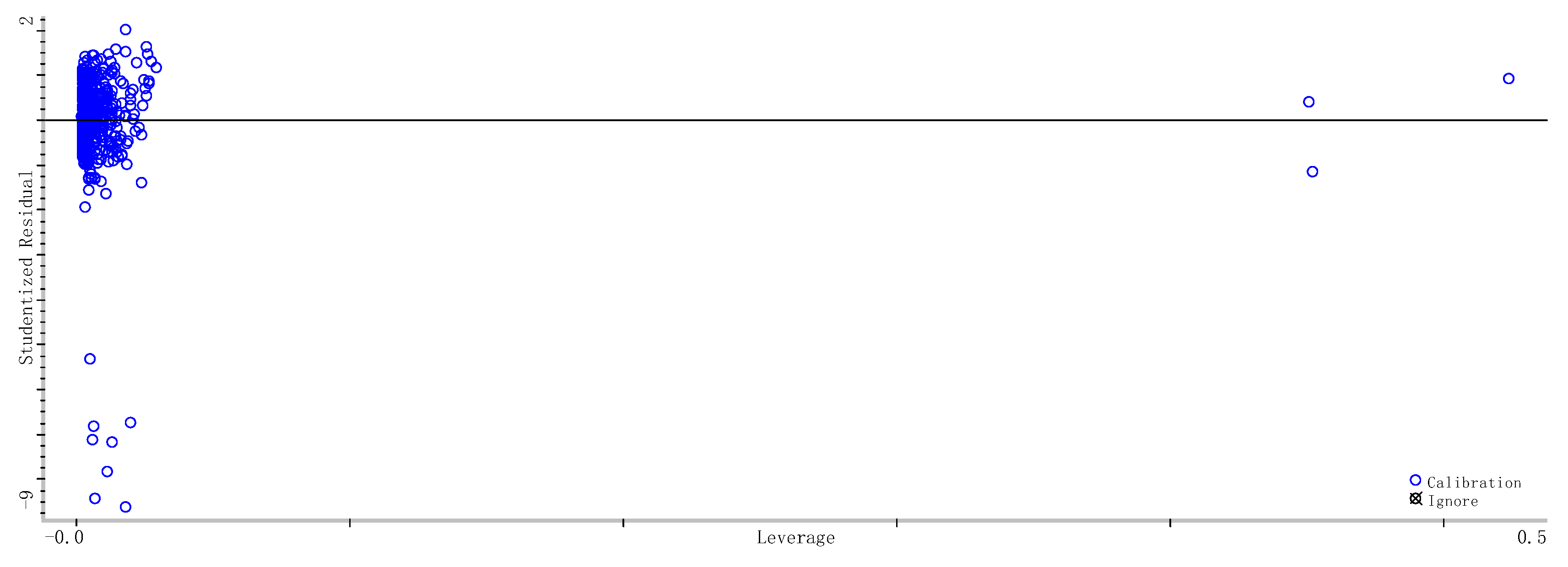
3.1.1. Outlier Samples Rejection
3.1.2. Spectral Data Preprocessing
3.1.3. Spectral Dimensionality Reduction
3.2. Traditional Modeling Methods
3.3. SE-DenseNet
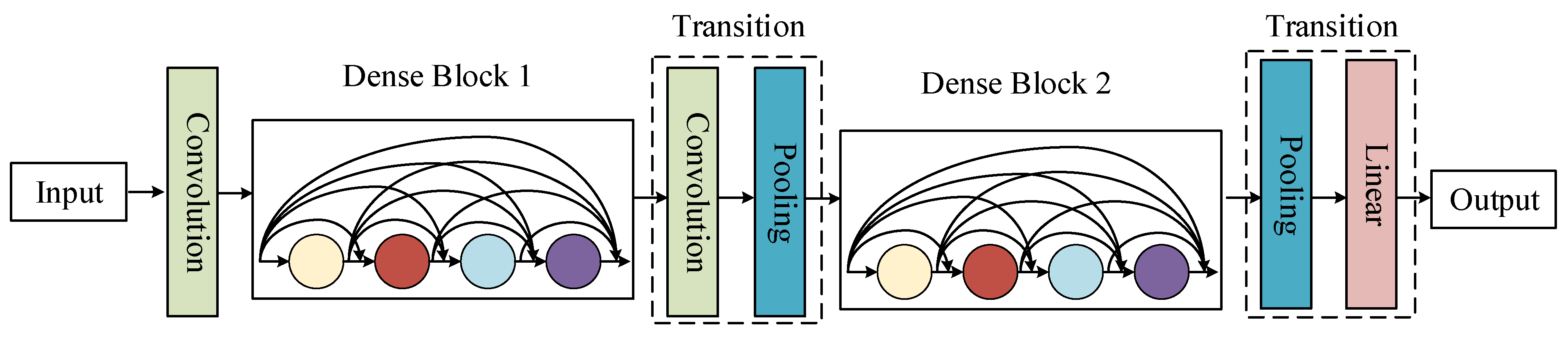
3.3.1. DenseNet
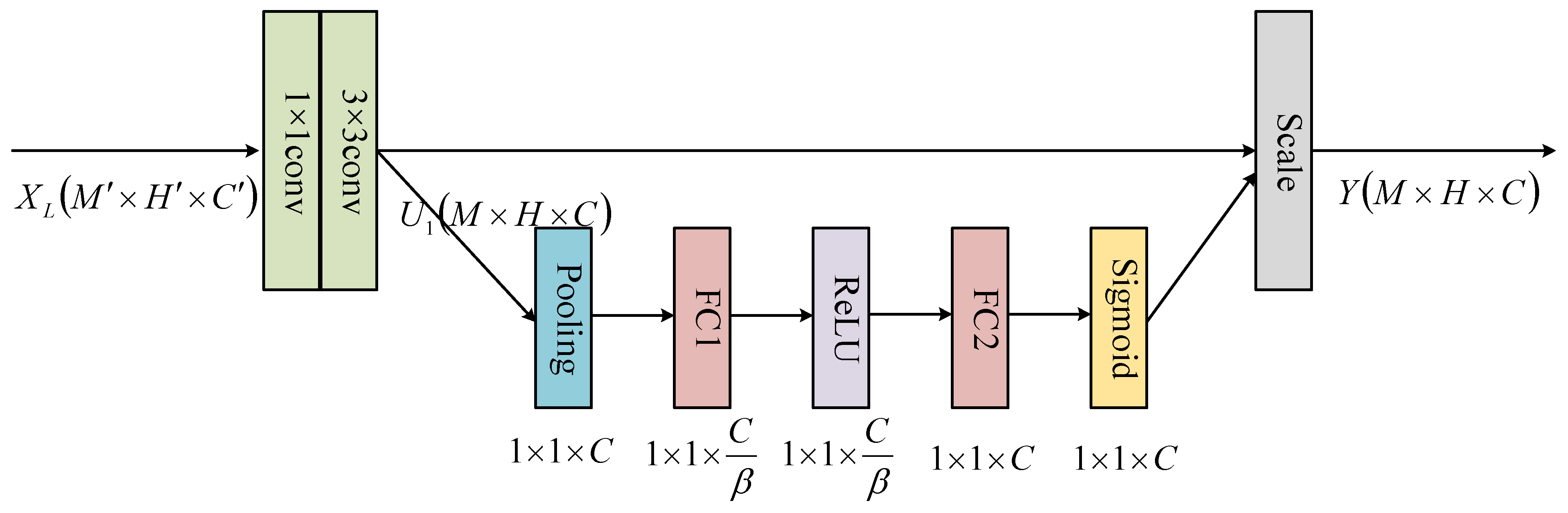
3.3.2. SE Module
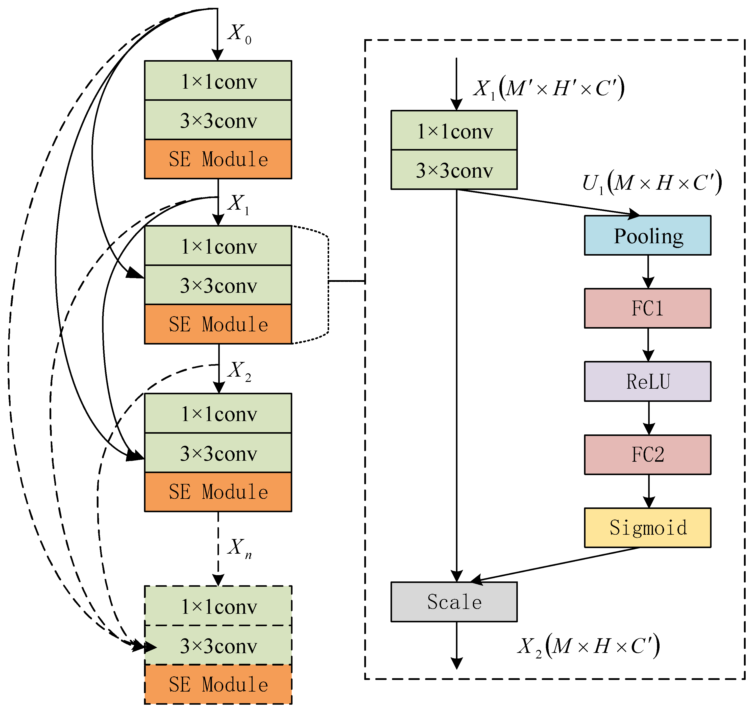
3.3.3. SE-DenseNet
3.4. Model Evaluation Index
4. Results and Discussion
4.1. Data Preprocessing Results
4.1.1. Outlier Sample Rejection Results
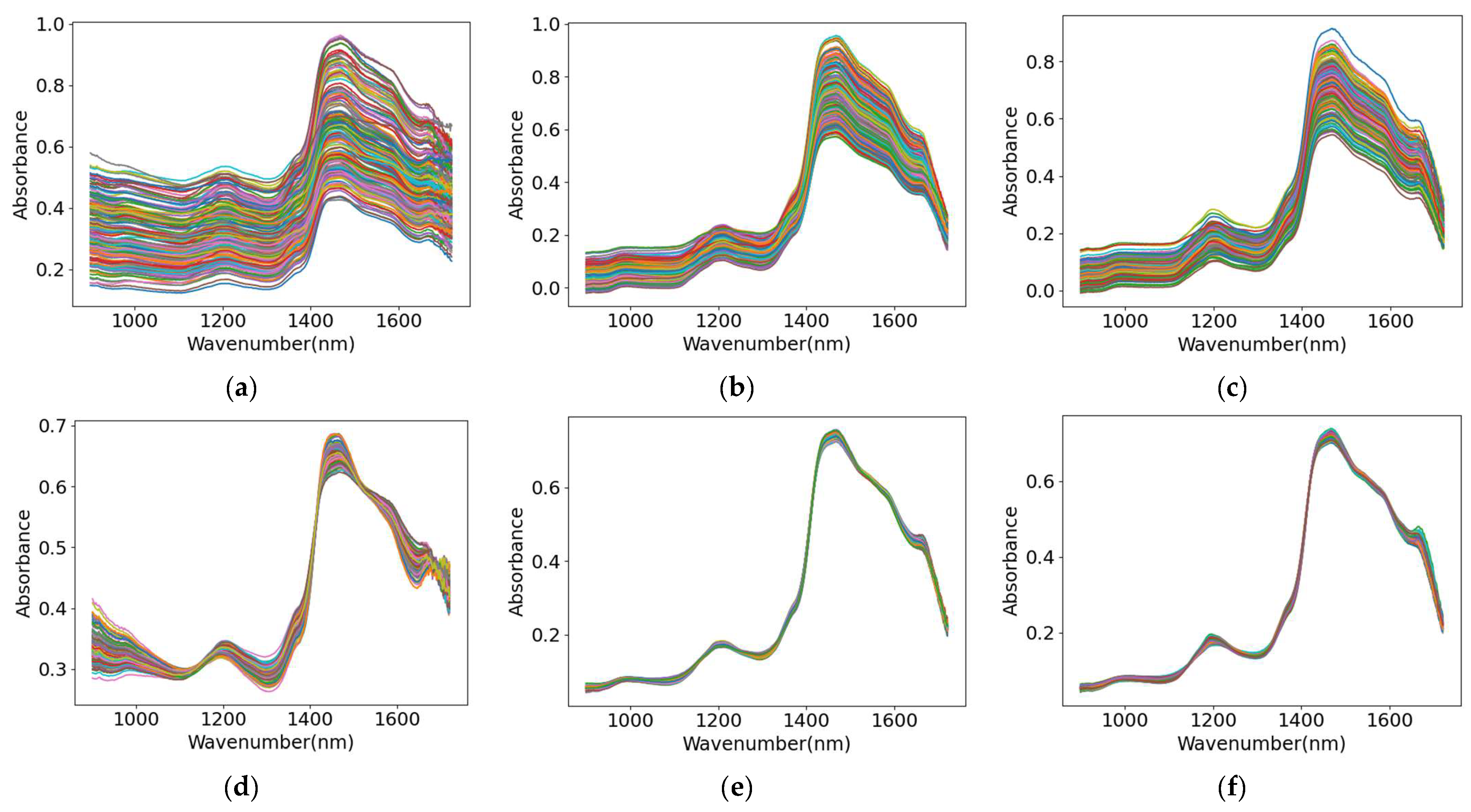
4.1.2. Spectral Preprocessing Results
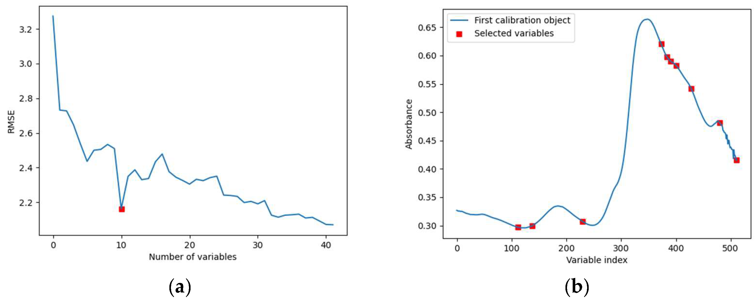
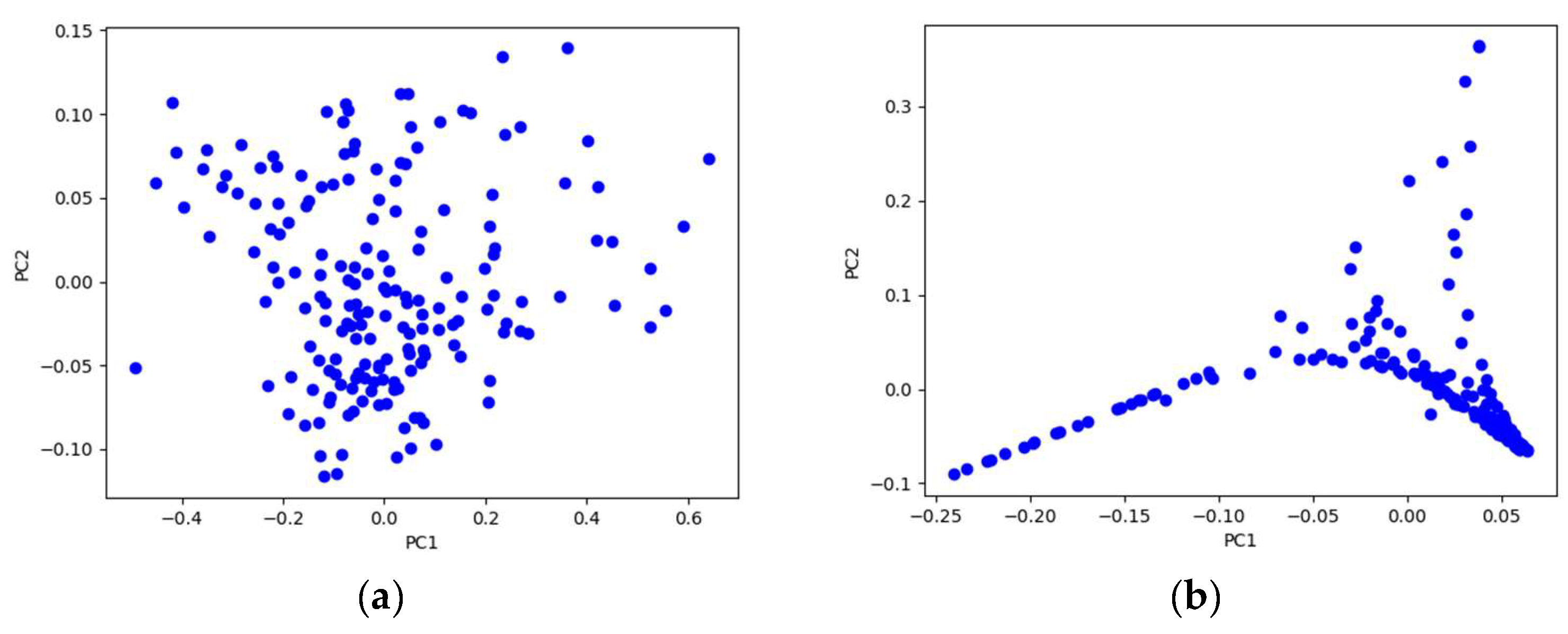
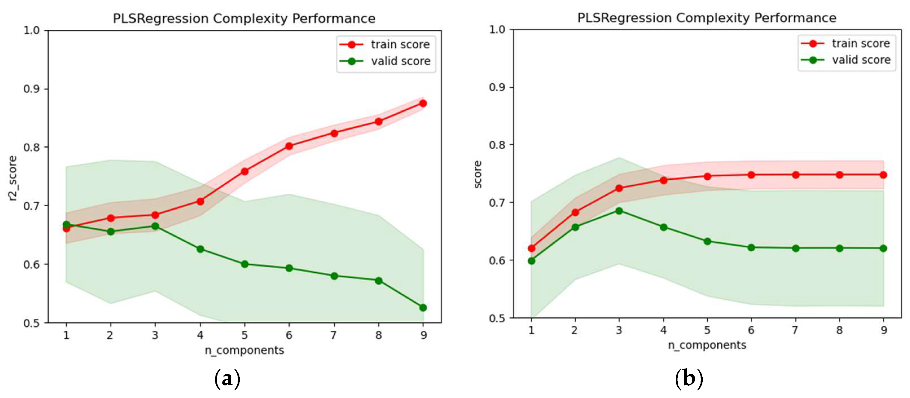
4.1.3. Spectral Dimensionality Reduction Results
4.2. Modeling Results
4.2.1. Classification of Coniferous Tree Species
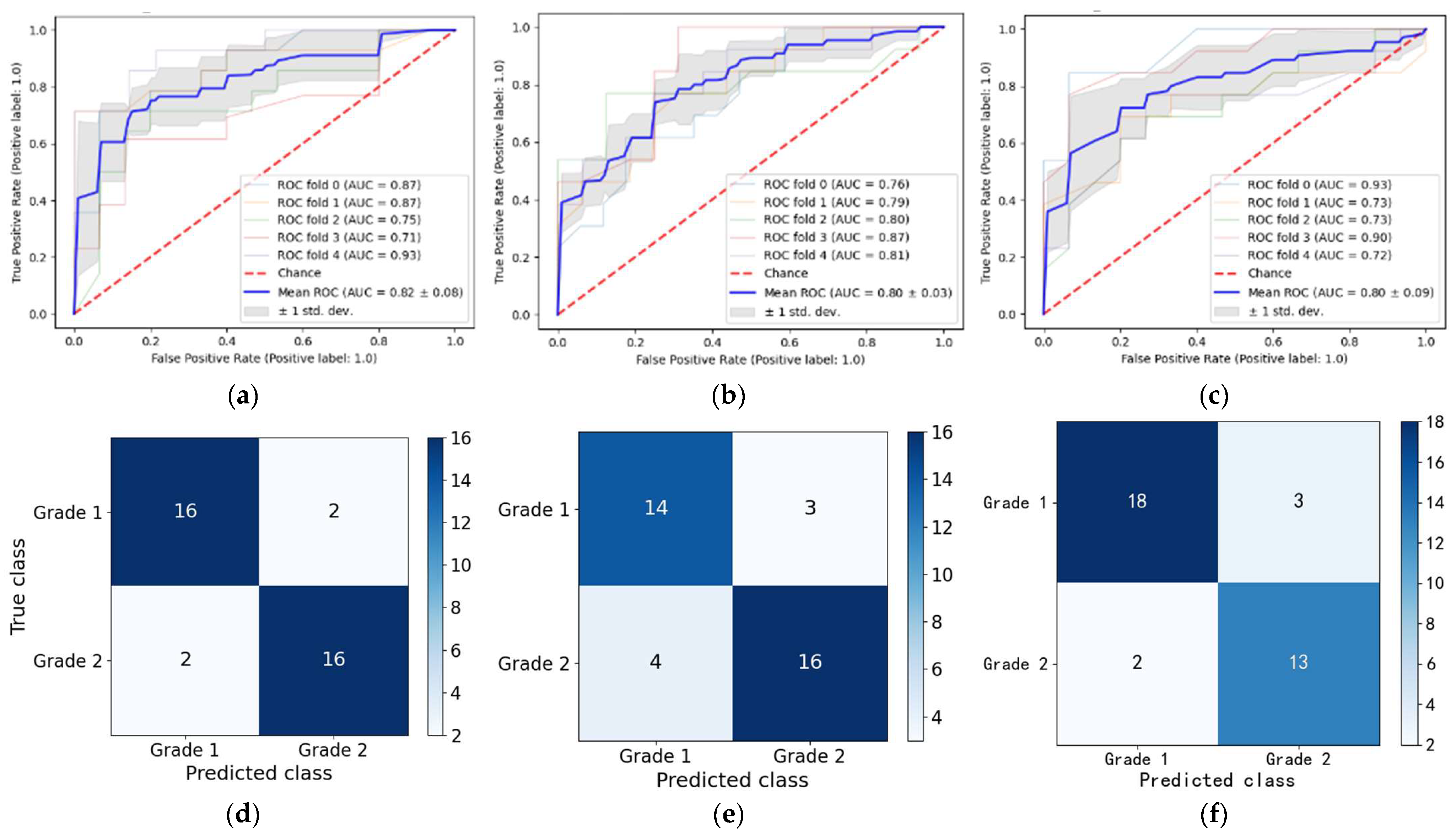
4.2.2. The Results of the Classification of the Mechanical Strength Level
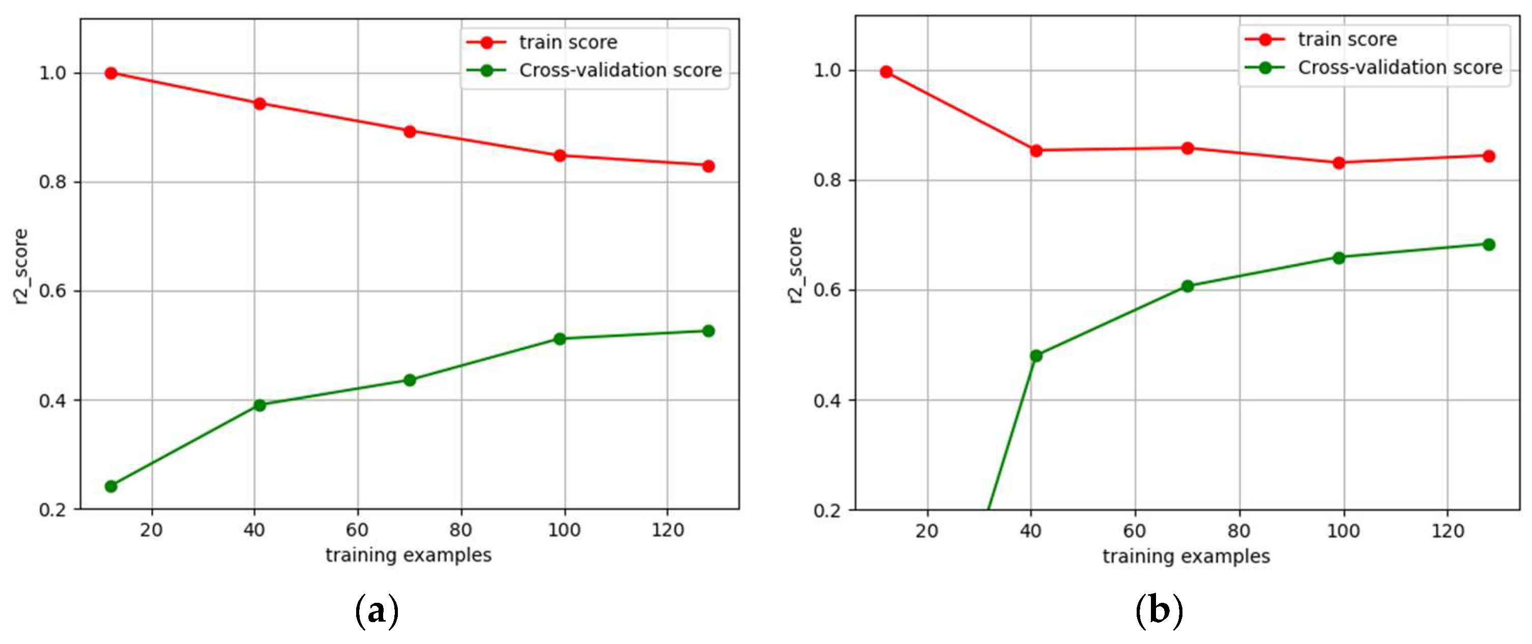
4.2.3. Numerical Regression Results of the Mechanical Strength
5. Conclusions
Author Contributions
Funding
Institutional Review Board Statement
Informed Consent Statement
Data Availability Statement
Acknowledgments
Conflicts of Interest
References
- Jia, R.; Lv, Z.H.; Wang, R.; Zhao, R.; Wang, Y. New advances in wood properties prediction by near-infrared spectroscopy. For. Ind. 2021, 58, 12–16+23. (In Chinese) [Google Scholar]
- Wang, X.P. Recent Advances in Nondestructive Evaluation of Wood: In-Forest Wood Quality Assessments. Forests 2021, 12, 949. [Google Scholar] [CrossRef]
- Schimleck, L.; Dahlen, J.; Apiolaza, L.A.; Downes, G.; Emms, G.; Evans, R.; Moore, J.; Pâques, L.; van den Bulcke, J.; Wang, X. Non-Destructive Evaluation Techniques and What They Tell Us about Wood Property Variation. Forests 2019, 10, 728. [Google Scholar] [CrossRef]
- Fang, Y.; Lin, L.; Feng, H.; Lu, Z.; Emms, G.W. Review of the use of air-coupled ultrasonic technologies for nondestructive testing of wood and wood products. Comput. Electron. Agric. 2017, 137, 79–87. [Google Scholar] [CrossRef]
- Yang, Z.; Jiang, Z.; Hse, C.Y.; Liu, R. Assessing the impact of wood decay fungi on the modulus of elasticity of slash pine (Pinus elliottii) by stress wave non- destructive testing. Int. Biodeterior. Biodegrad. 2017, 117, 123–127. [Google Scholar] [CrossRef]
- Lechner, T.; Sandin, Y.; Kliger, R. Assessment of density in timber using X-ray equipment. Int. J. Archit. Herit. 2013, 7, 416–433. [Google Scholar] [CrossRef]
- Tsuchikawa, S.; Ma, T.; Inagaki, T. Application of near-infrared spectroscopy to agriculture and forestry. Anal. Sci. 2022, 38, 635–642. [Google Scholar] [CrossRef]
- Wang, Y.; Xiang, J.; Tang, Y.; Chen, W.; Xu, Y. A review of the application of near-infrared spectroscopy (NIRS) in forestry. Appl. Spectrosc. Rev. 2022, 57, 300–317. [Google Scholar] [CrossRef]
- Beć, K.B.; Huck, C.W. Breakthrough potential in near-infrared spectroscopy: Spectra simulation. A review of recent developments. Front. Chem. 2019, 7, 48. [Google Scholar] [CrossRef]
- Ayanleye, S.; Nasir, V.; Avramidis, S.; Cool, J. Effect of wood surface roughness on prediction of structural timber properties by infrared spectroscopy using ANFIS, ANN and PLS regression. Eur. J. Wood Wood Prod. 2021, 79, 101–115. [Google Scholar] [CrossRef]
- Mancini, M.; Leoni, E.; Nocetti, M.; Urbinati, C.; Duca, D.; Brunetti, M.; Toscano, G. Near infrared spectroscopy for assessing mechanical properties of Castanea sativa wood samples. J. Agric. Eng. 2019, 50, 191–197. [Google Scholar] [CrossRef]
- Liang, H.; Zhang, M.; Gao, C.; Zhao, Y. Non-Destructive Methodology to Determine Modulus of Elasticity in Static Bending of Quercus mongolica Using Near- Infrared Spectroscopy. Sensors 2018, 18, 1963. [Google Scholar] [CrossRef]
- Wang, H.P.; Chen, P.; Dai, J.W.; Liu, D.; Li, J.Y.; Xu, Y.P.; Chu, X.L. Recent advances of chemometric calibration methods in modern spectroscopy: Algorithms, strategy, and related issues. TrAC Trends Anal. Chem. 2022, 153, 116648. [Google Scholar] [CrossRef]
- Mishra, P.; Passos, D.; Marini, F.; Xu, J.; Amigo, J.M.; Gowen, A.A.; Jansen, J.J.; Biancolillo, A.; Roger, J.M.; Rutledge, D.N.; et al. Deep learning for near-infrared spectral data modelling: Hypes and benefits. TrAC Trends Anal. Chem. 2022, 157, 116804. [Google Scholar] [CrossRef]
- Le, B.T. Application of deep learning and near infrared spectroscopy in cereal analysis. Vib. Spectrosc. 2020, 106, 103009. [Google Scholar] [CrossRef]
- Chen, Y.; Bin, J.; Zou, C.; Ding, M. Discrimination of fresh tobacco leaves with different maturity levels by near-infrared (NIR) spectroscopy and deep learning. J. Anal. Methods Chem. 2021, 2021, 9912589. [Google Scholar] [CrossRef]
- Yang, J.; Wang, J.; Lu, G.; Fei, S.; Yan, T.; Zhang, C.; Lu, X.; Yu, Z.; Li, W.; Tang, X. TeaNet: Deep learning on Near-Infrared Spectroscopy (NIR) data for the assurance of tea quality. Comput. Electron. Agric. 2021, 190, 106431. [Google Scholar] [CrossRef]
- Xu, Z.; Zhao, X.; Guo, X.; Guo, J. Deep learning application for predicting soil organic matter content by VIS-NIR spectroscopy. Comput. Intell. Neurosci. 2019, 2019, 3563761. [Google Scholar] [CrossRef]
- Zou, L.; Liu, W.; Lei, M.; Yu, X. An Improved Residual Network for Pork Freshness Detection Using Near-Infrared Spectroscopy. Entropy 2021, 23, 1293. [Google Scholar] [CrossRef]
- GB/T 1935-2009; Test Method for Longitudinal Compressive Strength of Wood. National Standards of People’s Republic of China: Beijing, China, 2009.
- GB/T 37969-2019; General Principles for Qualitative Analysis of Near-Infrared Spectroscopy. National Standards of People’s Republic of China: Beijing, China, 2019.
- GB/T 29858-2013; General Principles for Quantitative Analysis of Molecular Spectral Multivariate Correction. National Standards of People’s Republic of China: Beijing, China, 2013.
- Bian, X. Spectral Preprocessing Methods. In Chemometric Methods in Analytical Spectroscopy Technology; Springer: Singapore, 2022; pp. 111–168. [Google Scholar]
- Zebari, R.; AbdulAzeez, A.; Zeebaree, D.; Zebari, D.; Saeed, J. A comprehensive review of dimensionality reduction techniques for feature selection and feature extraction. J. Appl. Sci. Technol. Trends 2020, 1, 56–70. [Google Scholar] [CrossRef]
- Xing, Z.; Du, C.; Shen, Y.; Ma, F.; Zhou, J. A method combining FTIR-ATR and Raman spectroscopy to determine soil organic matter: Improvement of prediction accuracy using competitive adaptive reweighted sampling (CARS). Comput. Electron. Agric. 2021, 191, 106549. [Google Scholar] [CrossRef]
- Zhang, D.Y.; Jiang, D.P.; Zhou, B.L.; Cao, J.; Zhao, S.Q. Local linear embedding based on flow learning for near-infrared detection of red pine nut quality. J. Northeast. For. Univ. 2019, 47, 45–48. (In Chinese) [Google Scholar]
- Raghavendra, A.; Guru, D.S.; Rao, M.K. Mango internal defect detection based on optimal wavelength selection method using NIR spectroscopy. Artif. Intell. Agric. 2021, 5, 43–51. [Google Scholar] [CrossRef]
- Chu, X. Chemometric Methods in Modern Spectral Analysis; Chemical Industry Press: Beijing, China, 2022; pp. 176–197. [Google Scholar]
- Zhu, Y.; Newsam, S. Densenet for dense flow. In Proceedings of the 2017 IEEE International Conference on Image Processing (ICIP), Beijing, China, 17–20 September 2017; IEEE: Piscataway, NJ, USA, 2017; pp. 790–794. [Google Scholar]
- Hu, J.; Shen, L.; Sun, G. Squeeze-and-excitation networks. In Proceedings of the IEEE Conference on Computer Vision and Pattern Recognition, Salt Lake City, UT, USA, 18–23 June 2018; pp. 7132–7141. [Google Scholar]
- Yun, Y.H. Method of Selecting Calibration Samples. In Chemometric Methods in Analytical Spectroscopy Technology; Springer: Singapore, 2022; pp. 297–308. [Google Scholar]
- Yang, Y.; Zhao, C.; Huang, W.; Tian, X.; Fan, S.; Wang, Q.; Li, J. Optimization and compensation of models on tomato soluble solids content assessment with online Vis/NIRS diffuse transmission system. Infrared Phys. Technol. 2022, 121, 104050. [Google Scholar] [CrossRef]
- Huang, L.; Wu, K.; Huang, W.; Dong, Y.; Ma, H.; Liu, Y.; Liu, L. Detection of fusarium head blight in wheat ears using continuous wavelet analysis and PSO-SVM. Agriculture 2021, 11, 998. [Google Scholar] [CrossRef]
- Wang, L.; Wang, R. Determination of soil pH from Vis-NIR spectroscopy by extreme learning machine and variable selection: A case study in lime concretion black soil. Spectrochim. Acta Part A Mol. Biomol. Spectrosc. 2022, 283, 121707. [Google Scholar] [CrossRef]


| Network Layer | SE-DenseNet | DenseNet | ||
|---|---|---|---|---|
| Matrix Dimensions | Structure Configuration | Matrix Dimensions | Structure Configuration | |
| Convolution | n × n | [3 × 3, 2c] | n × n | [3 × 3, 2c] |
| Pooling | — | — | n/2 × n/2 | 3 × 3 Max pooling |
| Block of structure | n × n | n/2 × n/2 | ||
| Transition Layer | n × n | [1 × 1, 0.5c] | n/2 × n/2 | [1 × 1, 0.5c] |
| n/4 × n/4 | 2 × 2 Average pooling | |||
| Classification Layer | 1 × 1 | Global average pool, Fully-connected, softmax | ||
| Predicted Class | ||||||
|---|---|---|---|---|---|---|
| 1 | 2 | 3 | G | |||
| Actual class | 1 | |||||
| 2 | ||||||
| 3 | ||||||
| G | ||||||
| Predicted Class | |||
|---|---|---|---|
| Positive | Negative | ||
| Actual class | Positive | TP | FN |
| Negative | FP | TN | |
| Pretreatment Method | Cross-Validation Set | Test Set | ||
|---|---|---|---|---|
| RMSECV: MPa | RCV | RMSEP: MPa | RP | |
| Original spectrum | 3.6918 | 0.5594 | 3.9972 | 0.5157 |
| D2 + WT + MSC + VN | 6.6329 | 0.0318 | 6.2443 | 0.1465 |
| WT + MSC + VN | 2.4617 | 0.7354 | 2.4609 | 0.7359 |
| D1 + WT + MSC | 5.1621 | 0.4291 | 5.6343 | 0.3716 |
| WT + MSC | 2.2640 | 0.7550 | 2.3660 | 0.7453 |
| WT + SNV | 2.3657 | 0.7455 | 2.4513 | 0.7373 |
| WT | 3.2146 | 0.6294 | 3.3429 | 0.6174 |
| SG | 3.2519 | 0.6289 | 3.3876 | 0.6162 |
| SG + MSC | 2.5960 | 0.7278 | 2.5145 | 0.7317 |
| Methods | Number of Features | Cross-Validation Set | Test Set | ||
|---|---|---|---|---|---|
| RMSECV: MPa | RCV | RMSEP: MPa | RP | ||
| SPA | 10 | 1.9881 | 0.7879 | 2.0378 | 0.7852 |
| CARS | 66 | 1.9006 | 0.8106 | 1.9158 | 0.8033 |
| PCA | 10 | 2.0214 | 0.7852 | 2.0554 | 0.7827 |
| LLE | 7 | 1.9121 | 0.8078 | 1.9189 | 0.8025 |
| CARS + PCA | 13 | 1.7293 | 0.8319 | 1.6970 | 0.8382 |
| CARS + LLE | 6 | 1.6031 | 0.8523 | 1.6658 | 0.8498 |
| Range of Values | Grade 1: MPa | Grade 2: MPa |
|---|---|---|
| larch | 54.9–64.8 | 64.8–78.6 |
| hemlock | 40.2–52.3 | 52.3–59.8 |
| mongolica | 35.2–46.2 | 46.2–52.4 |
| Tree Species | Methods | Cross-Validation Set | Test Set | ||
|---|---|---|---|---|---|
| ACCCV | F1CV | ACCP | F1P | ||
| larch | WT + MSC, CARS + LLE, PLS-DA | 0.7931 | 0.7752 | 0.7777 | 0.7498 |
| WT + MSC, CARS + LLE, SVM | 0.8276 | 0.8142 | 0.8333 | 0.8267 | |
| WT + MSC, CARS + LLE, RF | 0.8540 | 0.8379 | 0.8333 | 0.8267 | |
| WT + MSC, DenseNet | 0.8342 | 0.8328 | 0.8540 | 0.8454 | |
| WT + MSC, SE-DenseNet | 0.8611 | 0.8601 | 0.8889 | 0.8831 | |
| hemlock | WT + MSC, CARS + LLE, PLS-DA | 0.7688 | 0.7624 | 0.7543 | 0.7499 |
| WT + MSC, CARS + LLE, SVM | 0.7854 | 0.7745 | 0.7637 | 0.7591 | |
| WT + MSC, CARS + LLE, RF | 0.8065 | 0.8012 | 0.7965 | 0.7825 | |
| WT + MSC, DenseNet | 0.7854 | 0.7729 | 0.7965 | 0.7876 | |
| WT + MSC, SE-DenseNet | 0.8276 | 0.8201 | 0.8108 | 0.8016 | |
| mongolica | WT + MSC, CARS + LLE, PLS-DA | 0.7462 | 0.7387 | 0.7354 | 0.7321 |
| WT + MSC, CARS + LLE, SVM | 0.7688 | 0.7539 | 0.7428 | 0.7456 | |
| WT + MSC, CARS + LLE, RF | 0.8067 | 0.7976 | 0.8142 | 0.8078 | |
| WT + MSC, DenseNet | 0.7928 | 0.7863 | 0.8142 | 0.8046 | |
| WT + MSC, SE-DenseNet | 0.8214 | 0.8159 | 0.8571 | 0.8381 | |
| Tree Species | Methods | Cross-Validation Set | Test Set | ||
|---|---|---|---|---|---|
| RMSECV: MPa | RCV | RMSEP: MPa | RP | ||
| larch | WT + MSC, CARS + LLE, PLSR | 1.6031 | 0.8523 | 1.6658 | 0.8498 |
| WT + MSC, CARS + LLE, SVR | 1.4019 | 0.8765 | 1.4165 | 0.8733 | |
| WT + MSC, CARS + LLE, ELM | 1.4302 | 0.8722 | 1.4387 | 0.8679 | |
| WT + MSC, DenseNet | 1.3371 | 0.8859 | 1.3582 | 0.8768 | |
| WT + MSC, SE-DenseNet | 1.2636 | 0.9107 | 1.2389 | 0.9144 | |
| hemlock | WT + MSC, CARS + LLE, PLSR | 1.6215 | 0.8485 | 1.6659 | 0.8368 |
| WT + MSC, CARS + LLE, SVR | 1.4348 | 0.8542 | 1.5274 | 0.8495 | |
| WT + MSC, CARS + LLE, ELM | 1.3852 | 0.8659 | 1.3518 | 0.8705 | |
| WT + MSC, DenseNet | 1.3055 | 0.8726 | 1.3243 | 0.8717 | |
| WT + MSC, SE-DenseNet | 1.1975 | 0.9117 | 1.2293 | 0.8957 | |
| mongolica | WT + MSC, CARS + LLE, PLSR | 1.4898 | 0.8577 | 1.5546 | 0.8465 |
| WT + MSC, CARS + LLE, SVR | 1.5364 | 0.8469 | 1.4966 | 0.8541 | |
| WT + MSC, CARS + LLE, ELM | 1.2895 | 0.8698 | 1.2991 | 0.8684 | |
| WT + MSC, DenseNet | 1.2128 | 0.9015 | 1.2376 | 0.8874 | |
| WT + MSC, SE-DenseNet | 1.1664 | 0.9207 | 1.2244 | 0.8950 | |
Disclaimer/Publisher’s Note: The statements, opinions and data contained in all publications are solely those of the individual author(s) and contributor(s) and not of MDPI and/or the editor(s). MDPI and/or the editor(s) disclaim responsibility for any injury to people or property resulting from any ideas, methods, instructions or products referred to in the content. |
© 2022 by the authors. Licensee MDPI, Basel, Switzerland. This article is an open access article distributed under the terms and conditions of the Creative Commons Attribution (CC BY) license (https://creativecommons.org/licenses/by/4.0/).
Share and Cite
Li, C.; Chen, X.; Zhang, L.; Wang, S. Determination of Coniferous Wood’s Compressive Strength by SE-DenseNet Model Combined with Near-Infrared Spectroscopy. Appl. Sci. 2023, 13, 152. https://doi.org/10.3390/app13010152
Li C, Chen X, Zhang L, Wang S. Determination of Coniferous Wood’s Compressive Strength by SE-DenseNet Model Combined with Near-Infrared Spectroscopy. Applied Sciences. 2023; 13(1):152. https://doi.org/10.3390/app13010152
Chicago/Turabian StyleLi, Chao, Xun Chen, Lixin Zhang, and Saipeng Wang. 2023. "Determination of Coniferous Wood’s Compressive Strength by SE-DenseNet Model Combined with Near-Infrared Spectroscopy" Applied Sciences 13, no. 1: 152. https://doi.org/10.3390/app13010152
APA StyleLi, C., Chen, X., Zhang, L., & Wang, S. (2023). Determination of Coniferous Wood’s Compressive Strength by SE-DenseNet Model Combined with Near-Infrared Spectroscopy. Applied Sciences, 13(1), 152. https://doi.org/10.3390/app13010152