1. Introduction
The weld quality has a direct impact on the performance and lifespan of welded components. Weld defects reduce the weld quality and deteriorate its properties, which is why they should be avoided. There are many approaches to reduce the occurrence of weld defects such as cracks, pores, lack of fusion or incomplete penetration. Therefore, an effective and efficient method of detection and analysis of weld defects is an important topic. To study the physical structure of metals, metallography is typically used for this purpose. After the preparation of the specimens, an expert has to identify the weld seam’s properties qualitatively. This evaluation of welds is done manually with the aid of software. The area is marked with lines, whereupon the program specifies it in accordance with the scale. This procedure is time-consuming, and the result depends on the operator. The software cannot reliably distinguish between cracks, pores and other microstructures. It looks for transitions from light to dark areas depending on the set limit, and it can only indicate the roundness of dark particles in bright unetched matrix. For better analysis and comparison between different welds, it is beneficial to describe the weld properties as scalar quantities. However, since the artificial intelligence is being applied more and more in research and industry, quantized values are needed, especially for machine learning. By determining the ratio of significant areas within a micrograph, the effects of parameter changes can be investigated better and compared to each other.
Researchers are gradually applying artificial intelligence to the field of laser welding, such as using the quality inspection system to achieve non-destructive weld measurement and defect detection [
1], in-process monitoring based on deep learning [
2] or using the semantic segmentation algorithm to detect weld defects in safety vents of power batteries [
3]. Long et al. [
4] opened the era of fully convolutional networks (FCN) for semantic segmentation. There are currently many variants of FCN-based models that have contributed to the exploration of semantic segmentation [
5,
6,
7,
8,
9]. Gyasi et al. provide an overview of the use of artificial intelligence in welding technology [
10]. Tantrapiwat describes a method of defect detection using a synthetic image dataset if a large number of input images on convolutional neural networks is not accessible [
11].
Due to the non-uniformity of the shape, position and size of weld defects, it is a complicated task to manually analyse and evaluate the recorded weld defect patterns. For example, cracks are sometimes wide and sometimes narrow, and there is no fixed standard for length. The pore is not always an ideal circle, and sometimes cracks and pores are connected. These are some of the difficulties in artificially distinguishing the types of weld defects. There are cases in which it is difficult to identify weld defects, such as identifying the boundary of the weld area from the fuzzy heat-affected zone. At the same time, a fair quantitative analysis is also particularly important for the evaluation of welding performance. Therefore, human participation is still always necessary for the analysis of complex weld defects. Hence, it is a very time-consuming and therefore expensive task.
This contribution provides a weld contour and weld defect identification and analysis based on a self-created data set. This leads to convenience for further research in the future. This preliminary work is used to create datasets suitable for processing with machine learning algorithms. From these, predictions can be made about weld quality under different parameter configurations. While many AI-based methods focus on real-time data during the welding process, the deep learning-based detection of structures in the micrographs simplifies the link between real-time data recorded during the welding process and the micrographs evaluated afterwards.
2. Methodology
There are many studies on laser weld defect detection. Since different studies require different data sets, a data set of deep welds has been created in order to broaden the application of deep learning in welding processes. It contains micrographs of different welding situations to ensure a wide range of applications in the field of weld property detection. The methodology includes obtaining the micrographs from welds, labeling the obtained micrographs, building the training environment of the neural network and quantifying and analyzing the prediction results.
2.1. Data Set Creation and Training Process
Round bars were welded on their circumference either in the form of a bead on plate welds or as dissimilar butt joints. The bars were rotated while a fixed laser beam was used for partial penetration welding. The detailed description of the experimental setup is available in [
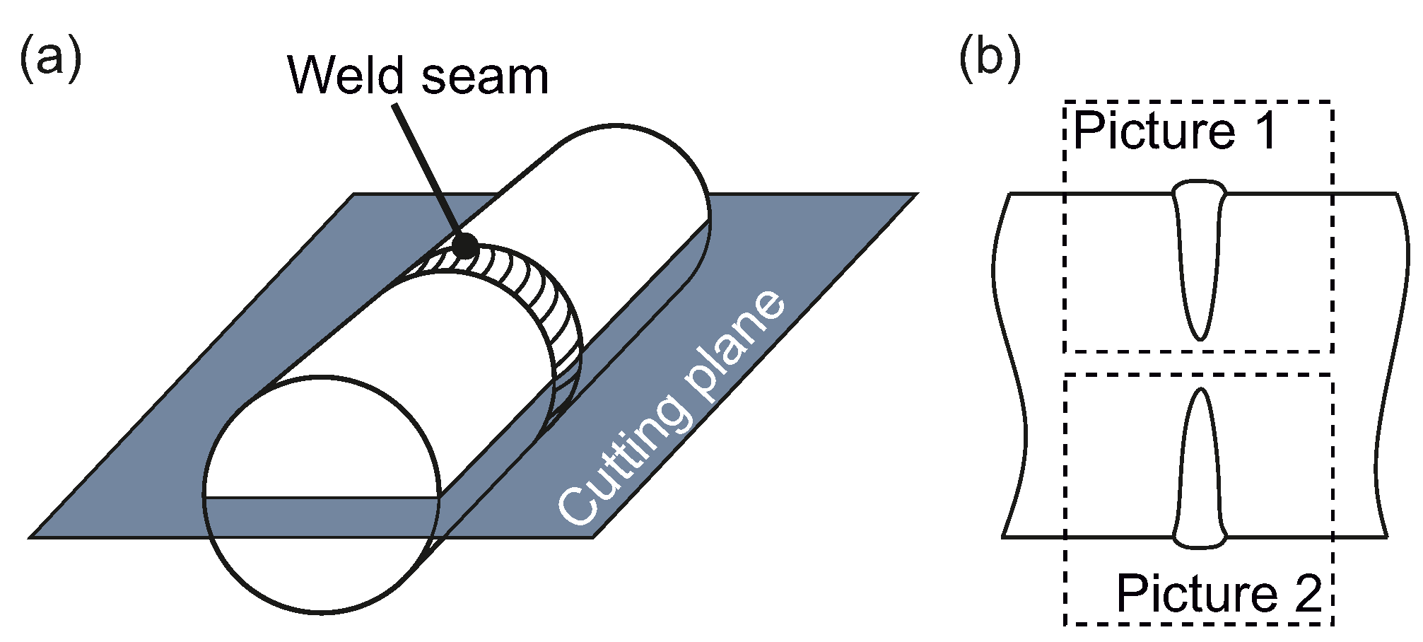
12]. After welding, the round bars were prepared for metallurgical investigations. Therefore, a cut was made longitudinally with the use of a wet cutting grinder; see
Figure 1a. After treatment with an etchant, two high-resolution micrographs were obtained out of one weld; see
Figure 1b. To ensure a proper training process, only welds whose weld depth did not reach the center of the round bars were used, since otherwise it is difficult to train the recognition of the outer contour of the weld.
The training process includes image preprocessing, image labeling, neural network training and automatic analysis of prediction results. In this work, the popular model DeepLabv3+ [
13] was used, which combines the advantages of multi-scale context information and spatial information, which is very suitable for the task, since the micrographs have weld defects of different shapes and sizes. Some weld defects are very small, which makes identification at high resolutions necessary. DeepLabv3+ combines multi-scale contextual information and rich spatial information. The model is already packaged in MATLAB [
14], and the corresponding backbone pre-trained network can be easily downloaded. All data were split into a training dataset, validation dataset and test dataset using random sampling, but in order to reproduce the results, the random seed was fixed. The training process was carried out with the created dataset using MATLAB version R2020a on a total of four GPUs of model 2080Ti and at least 160 GB of hard disc space reserved. The epochs were set to 50, which turned out to be large enough, because the accuracy of the model hardly changed as the epochs became larger than 20.
2.2. Preprocessing
Since the size and shape of each class in the micrographs are different and uncertain, in order to allow the neural network to learn the characteristics of each class and distinguish them sufficiently, it is necessary to make the model have a different receptive field. The “atrous spatial pyramid polling” (ASPP) in the DeepLabv3+ model solves this problem. Different dilation rates are used to extract features from images, which gives the model a good understanding of features of different sizes. The use of atrous or dilated convolution ensures that the receptive field is expanded without increasing computational pressure [
15]. In the traditional direct upsampling operation, semantic information and spatial information contradict each other. As the number of network layers increases, the feature map will gradually become smaller and the semantic information will become more and more abundant. One pixel covers more information from the original image, but it comes along with the loss of more spatial information. Making a reasonable weight distribution between semantic information and spatial information is very important. In the DeepLabv3+ model, Chen et al. [
13] introduced a novel decoder module, which is different from the traditional direct upsampling operation. The low-level feature map is cascaded with the output from the encoder that contains multi-scale rich semantic information.
2.3. Image Labeling
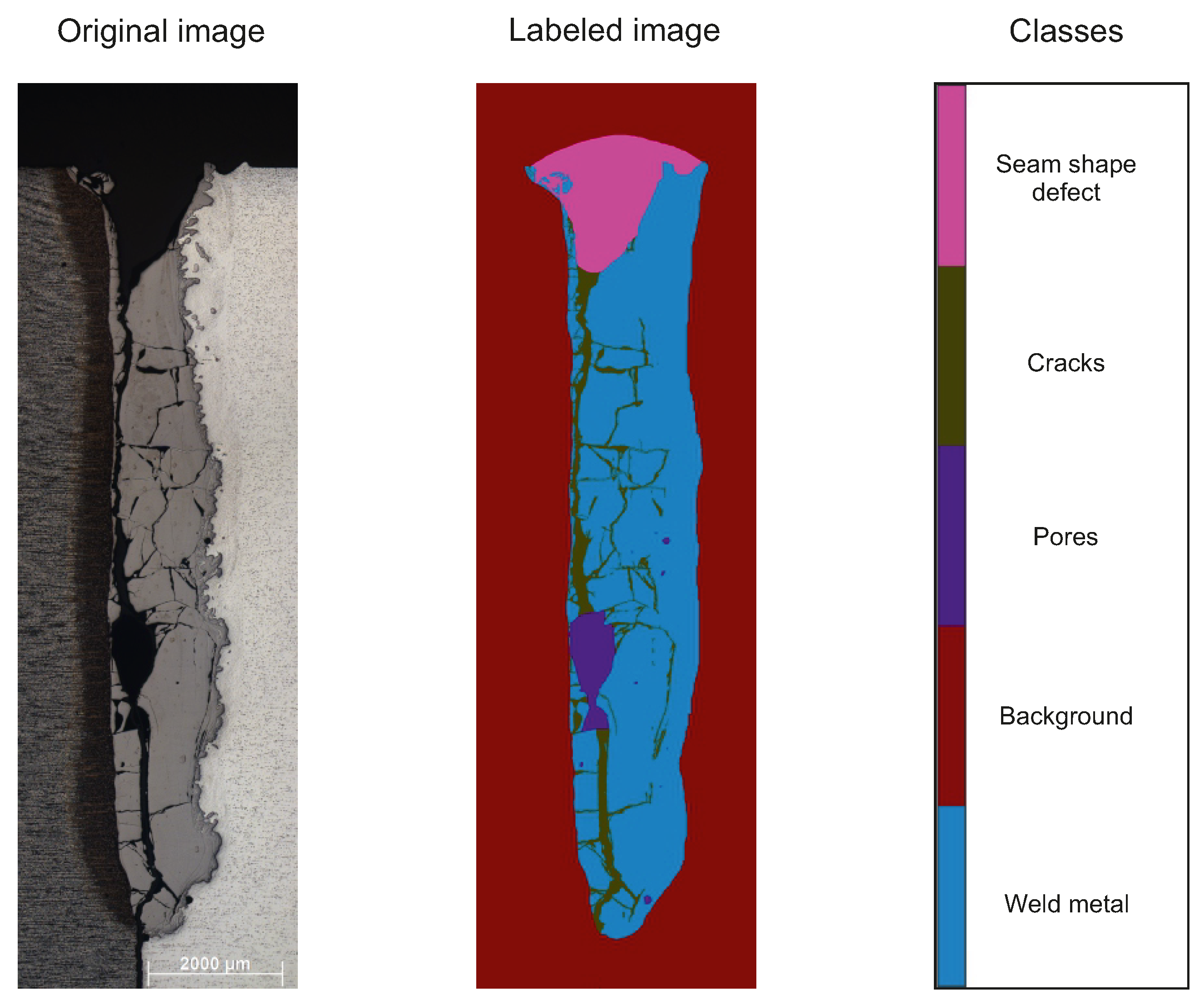
At present, the popular image labeling tools for computer vision are “labelme”, “labelImg” or “CVAT”. In this work, the image labeling tool “Image Labeler” that comes along with the MATLAB software was used. The semantic segmentation model used belongs to supervised learning. In order for the neural network to achieve better results in learning and to clearly identify weld defects and weld metal, each class was labeled. An original image and a labeled image are shown in
Figure 2. Both were used as input to the neural network. The original image was needed for the training of the neural network. Finally, the predicted segmented image was compared with the labeled image.
Five classes were initially defined for the classification, as follows:
The part inside the base material having a clear weld boundary belongs to the weld area, while the rest belongs to the background colored in red;
A weld reinforcement or sagging that causes a deviation in the expected weld seam shape requirements is defined as a seam shape defect. The label color is pink;
The remaining parts that are in the weld area without defects are weld metal. The label color of weld metal is blue;
If there is a long and thin weld defect within the weld area, it is defined as crack. The label color is green;
Weld defects formed like a bubble are defined as pores. The label color of pores is purple.
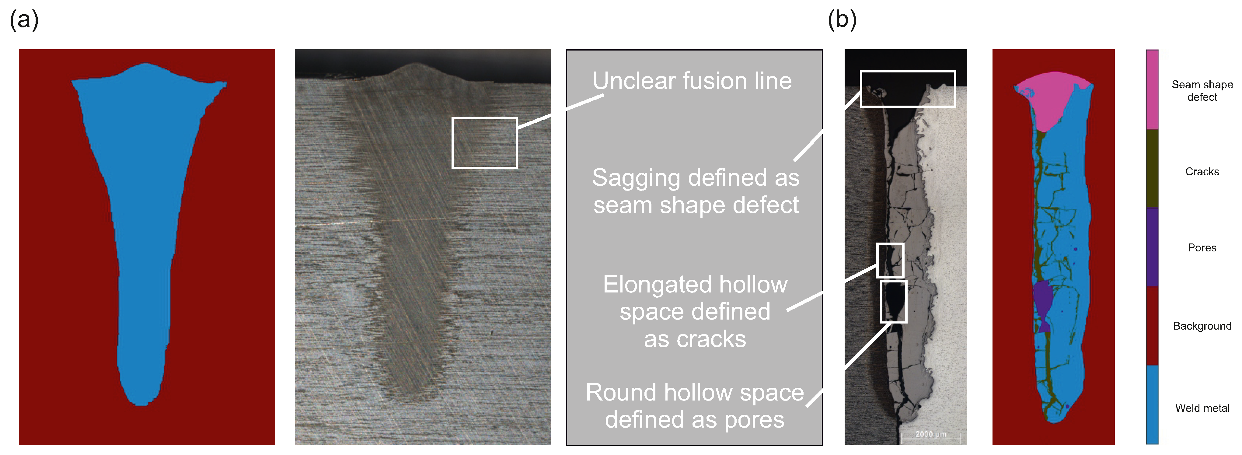
Since some defects are very small, image labeling is done pixel-by-pixel. Although there is a clear rule for image labeling, there is still the problem of ambiguous error in the process of image labeling, which can mainly be divided into the following three situations:
Ambiguous defects between weld metal and background:
From the original image in
Figure 3a, it can be seen that the fusion line of weld metal is difficult to distinguish from the background. The reason is that the colors of weld metal and base metal or heat affected zone are very similar, so no clear boundary can be obtained. In this case, image labeling requires enlarging the image to obtain a finer texture for an artificially based estimation of the position of the boundary;
Ambiguous defects between pores and cracks:
The purple label in
Figure 3b represents pores. According to the definition, pores are spherical cavities formed by gas inclusions. It should be spherical, but in the actual image labeling, it refers to voids that do not match the thin and long properties of cracks and which are located in the weld area;
Ambiguous defects between seam shape defects and the background:
The pink label stands for seam shape defects. Seam shape defects describe the deviation between the actual weld geometry and the expected weld geometry, but it is difficult to determine a fixed shape standard for a weld reinforcement. To solve this problem, in the case that the weld metal is higher than the base metal, it is assumed that there is no seam shape defect. In the case that the weld metal is lower than the base metal, the rest is artificially filled according to the shape of weld metal, forming a full arc.
2.4. Evaluation Methods
After training the segmentation model, the performance needs to be analysed. Although machine learning technology is advancing, every prediction result has errors. There are some types of evaluation methods that can used to perform a quantitative error consideration of the trained model. A better model can be attained only if the error analysis is continuously combined with the adjustment of the model parameters.
In the field of machine learning and statistical classification problems, the confusion matrix is a visualization tool especially for supervised learning. When evaluating standard machine learning models, the confusion matrix typically is used to divide predictions into four categories: true positives (
), false positives (
), true negatives (
) and false negatives (
). Taking the segmentation result 1 from
Section 4.1,
Table 1 results as an example of a confusion matrix. With this matrix, it is easy to see if the machine is confusing different classes. Each row of the confusion matrix represents the predicted category and each column represents the true category of the data.
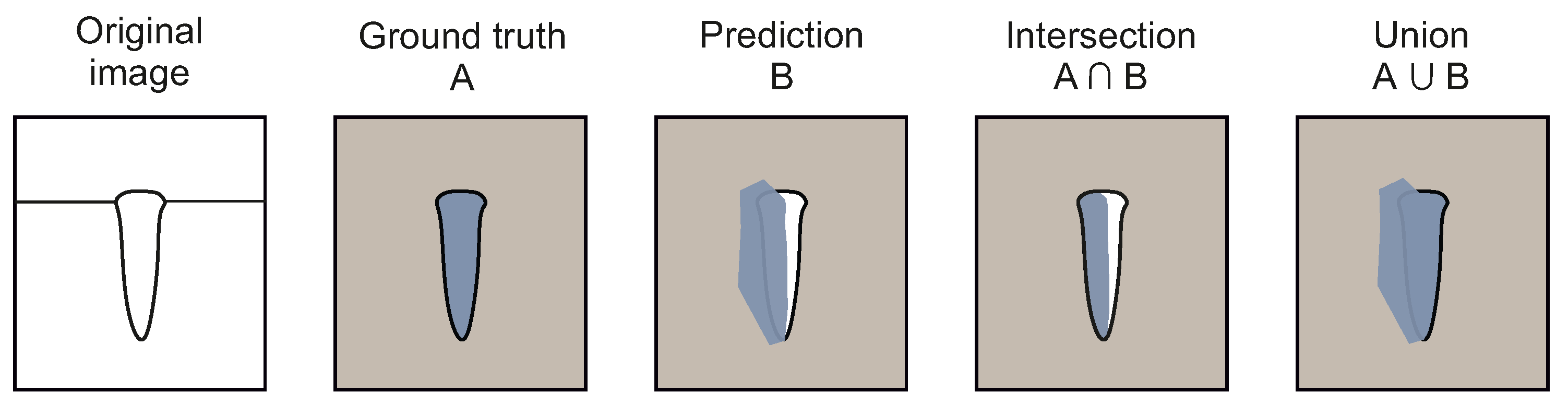
Using these categories, the Intersection over Union (IoU) can be calculated as the overlap rate between the prediction area generated by the model and the area of ground truth. This overlap rate can comprehensively account for the correctly predicted and incorrectly predicted pixels in the prediction results, which fully shows the credibility of the predicted results. It is therefore often used as an important evaluation criterion in the field of image semantic segmentation. The model can be evaluated using the following equations [
16,
17]:
As there are different methods used to evaluate the model, the results can be seen in
Table 2. Equation (
1) calculates the ratio of all correctly predicted pixels to all pixels. Equation (
2) calculates the probability of being correct among all outcomes predicted for a specific class. Equation (
3) calculates the ratio of the intersection of the predicted result and the ground truth to the union of the predicted result and the ground truth for a specific class, but it only considers all cases related to a specific class (TP, FP and FN), and it does not consider the positive effects brought by other classes (TN). As shown in
Table 1 with colored cells (TP = blue, FP = yellow, FN = green and TN = red), the use of Equation (
3) only considers the results in relation to a particular class. In order to evaluate the welds, the calculation method of Equation (
3) is chosen.
An example is given in
Figure 4 as a visual representation. It shows the ground truth and the predicted area as well as the intersection and the union between these two areas.
As multiple images are considered in general, the IoU of each image in the test set is averaged. Therefore, the “mean IoU” (
) is defined as shown in Equation (
4).
To analyse the IoU, the empirical mean and empirical variance are used. The empirical mean is the statistic obtained from one or more random variables, and the empirical variance is an estimate of the variance of the random variable based on the given sample.
2.5. Analysis Methods for Prediction Results
With the aid of the trained model, micrographs of laser-beam-welded, semi-finished products are automatically segmented semantically. Each pixel is assigned to a predicted class, which allows the resulting weld to be quantified. Firstly, the weld is analysed using the number of pixels corresponding to each weld defect. For example, the calculation for the ratio of pores is shown in Equation (
5).
With this calculation, it is possible to compare multiple pictures with different resolutions with each other as the predicted area is related in ratio to the size of the weld area.
3. Experimental Results
To evaluate the perfomance of the deep learning model, an ablation study was carried out. Therefore, the influence of different factors on the experimental results, the analysis of the final model and the achievements with the final model are described in detail.
3.1. Initialization of Weights
The essence of the deep learning model training process consists of updating the weights. Each parameter must have an appropriate initial value for network training. Poor initialization parameters can cause gradient propagation problems and reduce training speed, while good initialization parameters can speed up convergence and are more likely to find better solutions. In addition, the output of the middle layer of the model is intransparent, and the influence of the previous weights on the output of subsequent neurons is not unique. Even with such advanced parameter passing and updating, an inappropriate initialization of weights can cause laborious parameter learning and even the output loss gradient of the layer activation function to explode or vanish during forward propagation of the deep neural network. In either case, if the loss gradient is too large or too small, it cannot effectively backpropagate, and even if it can backpropagate, it takes longer for the network to reach convergence.
To ensure that low-frequency classes can be learned during the training process, weights were initialized according to the proportion of pixels occupied by each class in all images. The higher the proportion, the lower the initial weight of the class. Artificial adjustments were then made according to the results of the generated images. For example, if the class “cracks” was under-predicted, it was multiplied by a coefficient greater than one in the initial weight. Therefore, many different initial weights were tested. The best combination of initial weights in comparison with the unweighted combination is shown in
Table 3. In the case that the backbone was “Xception”, the result after adjustment was significantly improved. The initial weights from left to right stand for the weld metal, background, pores, cracks and seam shape defects.
3.2. Optimization Algorithm
The function of the optimization algorithm is to minimize or to maximize the loss function by improving the training method. When adjusting the weighting and deviation parameters for model updating, a suitable optimization algorithm can make the model achieve better and faster results. Due to the choice of the DeepLabv3+ model, three optimization algorithms were available: “SGDM”, “RMSprop” and “Adam”. Details of all optimization algorithms can be found in [
18].
To investigate the influence of the pre-trained network on the prediction result, a certain data set of micrographs was used with a variation of the network. From the neural network training results in
Table 4, it can be seen that the optimization algorithm of SGDM was more suitable for this project requirements, so SGDM was finally adopted.
3.3. Backbone
The backbone is a pre-trained network used by neural networks for simple feature extraction of the original image. In the Deeplabv3+ model, there are five pre-trained networks available, namely “ResNet-18”, “ResNet-50”, “MobileNet-v2”, “Xception” and “Inception-ResNet-v2”. The depth gradually increases from ResNet-18 to Inception-ResNet-v2, and the model needs to learn more parameters. The deeper the pre-trained network, the stronger the learning ability, but therefore the more training data that are needed. For the training process, an image resolution of 2048 × 1024 was used. The neural network was trained with different pre-trained networks with 169, images which is about 60% of the total amount of images of the data set. The results are shown in
Table 5.
3.4. Hyperparameter
Hyperparameters include the initial learning rate, the learning rate drop factor, the learning drop period and the regularization coefficient. Adjusting the hyperparameters is computationally intensive and time consuming. With “Xception” as a pre-trained network, two different hyperparameters were used to train the neural network. Specifically, the Nesterov momentum optimizer was parameterized with momentum = 0.9, initial learning rate = 0.05, learning rate drop factor = 0.94, learning drop period = 2 and regularization coefficient =
. The results are shown in
Table 6. After comparison, it can be found that hyperparameters have a great impact on the performance of the model.
3.5. Amount of Data for Training
Training data were used for the neural network model to learn the properties of each class. The larger the amount of training data, the stronger the ability for the neural network to generalize the properties of each class. An inadequate amount of data can easily lead to overfitting of the neural network because it cannot summarize the rules from more data. To improve the training accuracy, the neural network continuously adapts the model parameters to the characteristics of the training data set, which eventually leads to a high training accuracy, but the test accuracy is not ideal. As the training error decreases, the test error increases instead and overfitting occurs.
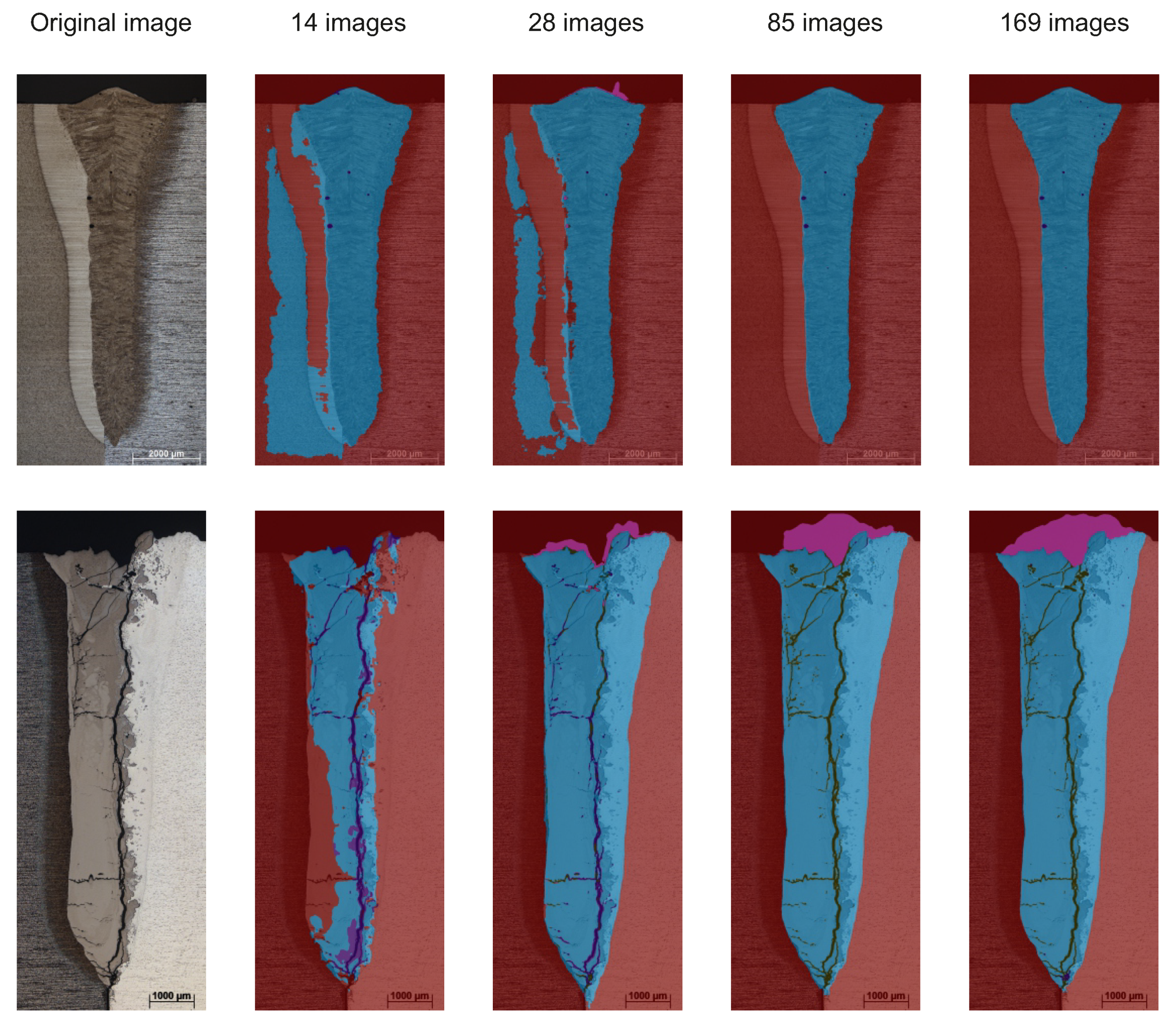
To evaluate the influence of the amount of data on the performance of the model, 5%, 10%, 30% and 60% of the total data were used as the training data set. The comparison results are shown in
Table 7.
Because the amount of 5% is very small, choosing this sample set randomly may lead to different results. To investigate this, the training was conducted with 10 runs in which the sample set was randomly selected from the total data. In this regard, a standard deviation of mIoU of 0.36% has been obtained.
Figure 5 shows two original images and the prediction results with different training sets. The larger the training set, the better the prediction results. An increase in the amount of training data improved the overall results. In this case, due to using a pre-trained network and because the change in performance is small in the range from 85 to 169 images, an amount of about 85 images already led to a good compromise between performance and calculation time. Whether a neural network can learn better in a particular detail cannot be answered by the amount of training data, but the more training data that are available, the more statistically significant and stable the training results are.
3.6. Image Resolution
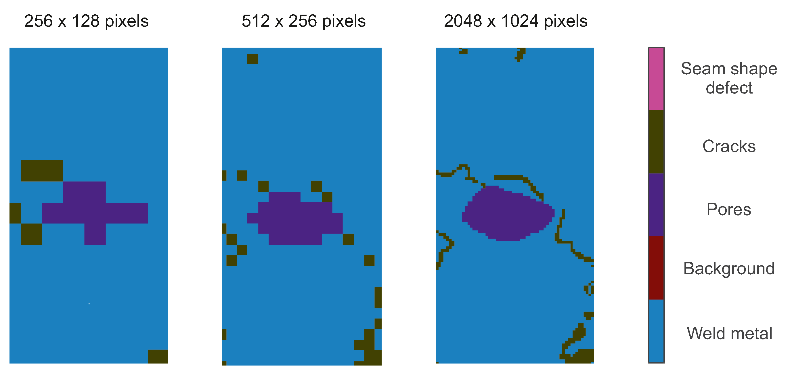
The image resolution used for neural network training is an important indicator that affects the performance. The micrographs used were high resolution images, and almost every image had a pixel count of 3000 × 2000. If the image is compressed, it is helpful to improve the training speed, but a too low resolution weakens or even destroys some features; see
Figure 6. A crack is a thin and long weld defect. If the resolution of the image is decreased to 512 × 256, most of the crack disappears. If the resolution is further changed to 256 × 128, almost all of the cracks are not learned. The target is to achieve a good balance of training speed and performance. According to the relationship between the side length of an image and the refinement quality investigated in [
19], images with a large resolution are important for the segmentation accuracy. For this reason, the resolution of 2048 × 1024 in this case comes along with a sufficient training speed while ensuring that all features are learned as well as possible.
4. Analysis of the Model
After studying the effect of different factors on the learning ability of neural networks, the DeepLabv3+ model achieved a performance of 76.88% of mIoU on the dataset. According to Equation (
3) the following quantitative values for the prediction classes can be obtained; see
Table 8 and
Table 9. The empirical mean and empirical variance of “Weld metal” and “Background” are better than the average, while the other classes are worse. Because of the bigger pixel count of the classes “Weld Metal” and “Background”, they are easier to learn in terms of appearance than the other classes.
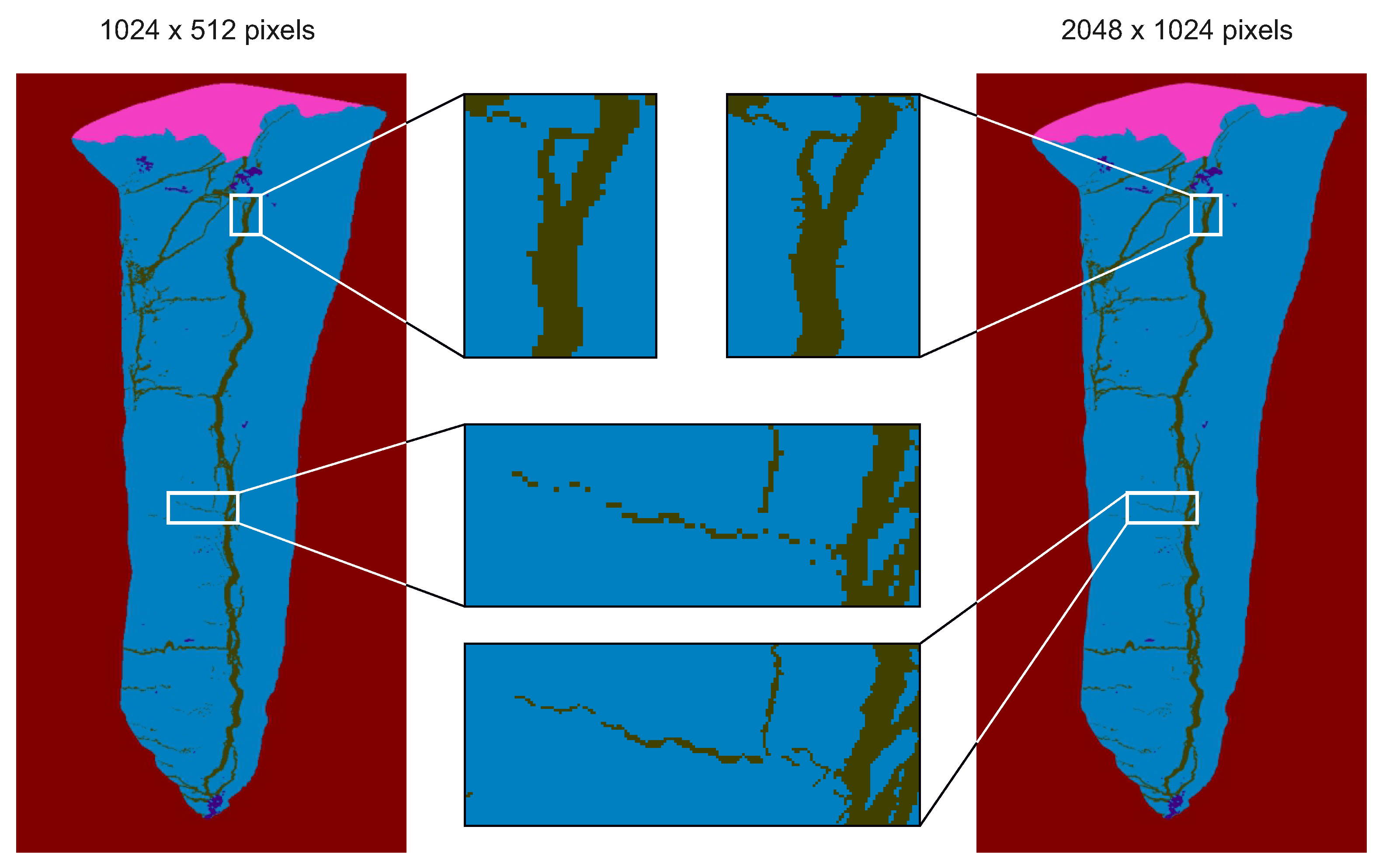
Comparing the two resolutions, it can be seen that a higher resolution leads to a more stable and accurate model. The comparison can be visualized by
Figure 7. This decrease in resolution does not seem to have much effect on the overall image, but details are going to be lost. With an enlargement of some areas, some loss of features can be seen, such as some cracks becoming less coherent.
4.1. Analysis of the Micrographs
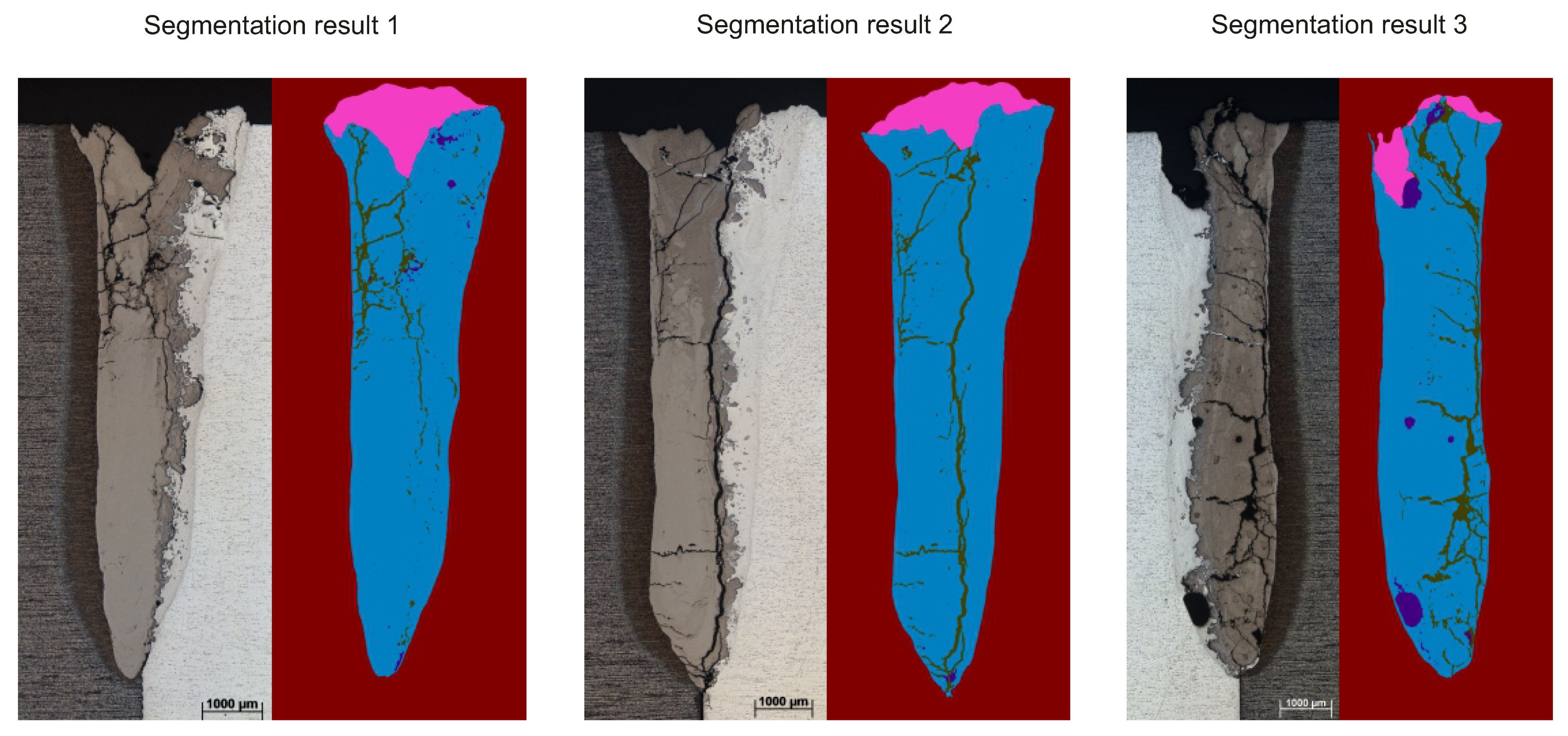
With the trained neural network a segmentation result of any micrograph can be parsed as shown in
Figure 8. Using the segmentation results, a determination of the pixel counts for each class is possible. The determined pixel counts reflect the severity of the weld defects and according to the IoU algorithm, the reliability of the segmentation results can be seen. The parsed results of
Figure 8 are shown in
Table 10.
With the aid of the standardized pixel numbers, the parsed results are comparable despite different scaling of the images. When the certain pixel numbers of defects are known, the ratio of each defect in the weld area can be calculated by Equation (
5). According to the data in
Table 10, the quantitative values given in
Table 11 are calculated. Afterwards, the different parsed results can be compared.
5. Conclusions
This contribution aims to introduce the current state-of-the-art deep learning techniques to detect weld metal and weld defects. A pre-trained neuronal network was trained and optimized according to the initialization of weights, optimization algorithm, backbone and hyperparameters. By pre-processing the data and adjusting the neural network model, a value of 76.88% of the mIoU was finally obtained for the defined classes. The neural network can automatically detect different areas within micrographs. The detection of weld metal has a high reliability, with an IoU of around 95%. Throughout the research process, a high-definition data set containing 282 images was created. It can be applied to any semantic segmentation model, which has significant implications for future research. Further research can continuously improve the neural network model based on the created data set to achieve better process improvement and quality assurance. With the automated detection of certain features within the weld area, it would also be possible to evaluate the quality of the welds. The results from the deep learning-based weld contour and defect detection could be compared with the established standards, such as DIN EN ISO 13919-1:2020-03, and the weld seam could be evaluated accordingly [
20].
Author Contributions
Conceptualization, C.N., T.G., J.G., S.N., J.T., J.H., S.K. and J.W.; methodology, C.N., T.G. and J.G.; software, C.N. and T.G.; validation, C.N., T.G. and J.G.; formal analysis, C.N., T.G. and J.G.; investigation, C.N., T.G. and J.G.; data curation, C.N., T.G., J.G. and S.N.; writing-original draft, C.N. and T.G.; writing—review and editing, C.N., T.G., J.G., S.N., J.T. and J.W.; visualization, C.N., T.G. and J.G.; supervision, J.W. and S.K.; project administration, C.N. and J.G.; funding acquisition, J.W. and S.K. All authors have read and agreed to the published version of the manuscript.
Funding
Funded by the Deutsche Forschungsgemeinschaft (DFG, German Research Foundation)—CRC 1153, subproject A3—252662854. The authors would like to thank them for the support.
Institutional Review Board Statement
Not applicable.
Informed Consent Statement
Not applicable.
Data Availability Statement
Some or all data generated or used during the study are available from the corresponding author by request.
Conflicts of Interest
The authors declare no conflict of interest.
References
- Nguyen, H.-C.; Lee, B.-R. Laser-vision-based quality inspection system for small-bead laser welding. Int. J. Precis. Eng. Manuf. 2014, 15, 415–423. [Google Scholar] [CrossRef]
- Knaak, C.; Kolter, G.; Schulze, F.; Kröger, M.; Abels, P. Deep learning-based semantic segmentation for in-process monitoring in laser welding applications. In Applications of Machine Learning; International Society for Optics and Photonics: San Diego, CA, USA, 2019; Volume 11139, p. 1113905. [Google Scholar]
- Zhu, Y.; Yang, R.; He, Y.; Ma, J.; Guo, H.; Yang, Y.; Zhang, L. A Lightweight Multiscale Attention Semantic Segmentation Algorithm for Detecting Laser Welding Defects on Safety Vent of Power Battery. IEEE Access 2021, 9, 39245–39254. [Google Scholar] [CrossRef]
- Long, J.; Shelhamer, E.; Darrell, T. Fully convolutional networks for semantic segmentation. In Proceedings of the IEEE Conference on Computer Vision and Pattern Recognition, Boston, MA, USA, 7–12 June 2015; pp. 3431–3440. [Google Scholar]
- Badrinarayanan, V.; Kendall, A.; Cipolla, R. Segnet: A deep convolutional encoder-decoder architecture for image segmentation. IEEE Trans. Pattern Anal. Mach. Intell. 2017, 39, 2481–2495. [Google Scholar] [CrossRef] [PubMed]
- Chen, L.C.; Papandreou, G.; Kokkinos, I.; Murphy, K.; Yuille, A.L. Semantic image segmentation with deep convolutional nets and fully connected crfs. arXiv 2014, arXiv:1412.7062. [Google Scholar]
- Zhao, H.; Shi, J.; Qi, X.; Wang, X.; Jia, J. Pyramid scene parsing network. In Proceedings of the IEEE Conference on Computer Vision and Pattern Recognition, Honolulu, HI, USA, 21–26 July 2017; pp. 2881–2890. [Google Scholar]
- Chen, L.C.; Papandreou, G.; Kokkinos, I.; Murphy, K.; Yuille, A.L. Deeplab: Semantic image segmentation with deep convolutional nets, atrous convolution, and fully connected crfs. IEEE Trans. Pattern Anal. Mach. Intell. 2017, 40, 834–848. [Google Scholar] [CrossRef] [PubMed] [Green Version]
- Chen, L.C.; Papandreou, G.; Schroff, F.; Adam, H. Rethinking atrous convolution for semantic image segmentation. arXiv 2017, arXiv:1706.05587. [Google Scholar]
- Gyasi, E.A.; Handroos, H.; Kah, P. Survey on artificial intelligence (AI) applied in welding: A future scenario of the influence of AI on technological, economic, educational and social changes. Procedia Manuf. 2019, 38, 702–714. [Google Scholar] [CrossRef]
- Tantrapiwat, A. Spot Welding Defect Detection Using Synthetic Image Dataset on Convolutional Neural Networks. In Proceedings of the 7th International Conference on Engineering, Applied Sciences and Technology (ICEAST), Pattaya, Thailand, 1–3 April 2021; pp. 16–19. [Google Scholar] [CrossRef]
- Ohrdes, H.; Nothdurft, S.; Nowroth, C.; Grajczak, J.; Twiefel, J.; Hermsdorf, J.; Kaierle, S.; Wallaschek, J. Influence of the ultrasonic vibration amplitude on the melt pool dynamics and the weld shape of laser beam welded EN AW-6082 utilizing a new excitation system for laser beam welding. Prod. Eng. 2021, 15, 151–160. [Google Scholar] [CrossRef]
- Chen, L.C.; Zhu, Y.; Papandreou, G.; Schroff, F.; Adam, H. Encoder-decoder with atrous separable convolution for semantic image segmentation. In Proceedings of the European Conference on Computer Vision, Munich, Germany, 8–14 September 2018; pp. 801–818. [Google Scholar]
- Semantic Segmentation Using Deep Learning. Available online: https://www.mathworks.com/help/vision/ug/semantic-segmentation-using-deep-learning.html (accessed on 27 September 2020).
- Yu, F.; Koltun, V. Multi-scale context aggregation by dilated convolutions. arXiv 2015, arXiv:1511.07122. [Google Scholar]
- Sokolova, M.; Japkowicz, N.; Szpakowicz, S. Beyond Accuracy, F-Score and ROC: A Family of Discriminant Measures for Performance Evaluation. In AI 2006: Advances in Artificial Intelligence. AI 2006. Lecture Notes in Computer Science; Sattar, A., Kang, B.H., Eds.; Springer: Berlin/Heidelberg, Germany, 2006; Volume 4304. [Google Scholar]
- Powers, D. Evaluation: From Precision, Recall and F-Factor to ROC, Informedness, Markedness & Correlation. Mach. Learn. Technol. 2008, 2, 37–63. [Google Scholar]
- Ruder, S. An overview of gradient descent optimization algorithms. arXiv 2016, arXiv:1609.04747. [Google Scholar]
- Cheng, H.K.; Chung, J.; Tai, Y.W.; Tang, C.K. CascadePSP: Toward Class-Agnostic and Very High-Resolution Segmentation via Global and Local Refinement. In Proceedings of the IEEE/CVF Conference on Computer Vision and Pattern Recognition, Seattle, WA, USA, 13–19 June 2020; pp. 8890–8899. [Google Scholar]
- ISO 13919-1:2019; Electron and Laser-Beam Welded Joints—Requirements and Recommendations on Quality Levels for Imperfections—Part 1: Steel, Nickel, Titanium and Their Alloys. International Organization for Standardization: Geneva, Switzerland, 2020.
Figure 1.
Obtaining images from welds: (a) Circumferential welds formed during welding of two cylindrical specimens cut as preparation for metallography. (b) Two micrographs resulting from metallography.
Figure 1.
Obtaining images from welds: (a) Circumferential welds formed during welding of two cylindrical specimens cut as preparation for metallography. (b) Two micrographs resulting from metallography.
Figure 2.
Original image, labeled image and class differentiation.
Figure 2.
Original image, labeled image and class differentiation.
Figure 3.
Ambiguous defects between weld metal and background (a), between porosity and cracks and seam shape defects and background (b).
Figure 3.
Ambiguous defects between weld metal and background (a), between porosity and cracks and seam shape defects and background (b).
Figure 4.
Ground truth and prediction area.
Figure 4.
Ground truth and prediction area.
Figure 5.
Prediction results depending on the amount of training data of 14 to 169 images.
Figure 5.
Prediction results depending on the amount of training data of 14 to 169 images.
Figure 6.
Comparison of labeled micrographs with different image resolutions.
Figure 6.
Comparison of labeled micrographs with different image resolutions.
Figure 7.
Comparison of prediction results with different image resolutions.
Figure 7.
Comparison of prediction results with different image resolutions.
Figure 8.
Segmentation results.
Figure 8.
Segmentation results.
Table 1.
Confusion matrix example for segmantation result 1; see
Section 4.1.
= blue,
= yellow,
= green and
= red.
Table 1.
Confusion matrix example for segmantation result 1; see
Section 4.1.
= blue,
= yellow,
= green and
= red.
| | Seam Shape Defect | Background | Pores | Cracks | Weld Metal |
|---|
| Seam shape defect | 661,478 pixels | 7327 pixels | 446 pixels | 13,065 pixels | 170 pixels |
| Background | 4415 pixels | 1,285,278 pixels | 0 pixels | 2 pixels | 1009 pixels |
| Pores | 1793 pixels | 41 pixels | 2318 pixels | 1541 pixels | 94 pixels |
| Cracks | 5413 pixels | 21 pixels | 3011 pixels | 25,964 pixels | 8 pixels |
| Weld metal | 878 pixels | 14,913 pixels | 0 pixels | 155 pixels | 67,812 pixels |
Table 2.
Comparison of different values calculated with the Equations (
1)–(
3) based on the confusion matrix in
Table 1.
Table 2.
Comparison of different values calculated with the Equations (
1)–(
3) based on the confusion matrix in
Table 1.
| Equation | (1) | (2) | (3) |
|---|
| Value | 97.41% | 80.96% | 79.74% |
Table 3.
Comparison of training results with different initial weights.
Table 3.
Comparison of training results with different initial weights.
| Initial Weights | Backbone | Image Resolution | mIoU |
|---|
| 1, 1, 1, 1, 1 | Xception | 2048 × 1024 | 60.96% |
| 0.95, 1.14, 0.15, 0.014, 0.062 | Xception | 2048 × 1024 | 76.88% |
Table 4.
Comparison of training results with different optimization algorithms.
Table 4.
Comparison of training results with different optimization algorithms.
| Optimization Algorithm | Backbone | Image Resolution | mIoU |
|---|
| SGDM | Xception | 2048 × 1024 | 76.88% |
| RMSprop | Xception | 2048 × 1024 | 17.40% |
| Adam | Xception | 2048 × 1024 | 38.08% |
Table 5.
Comparison of results with different pre-trained networks with improved parameters.
Table 5.
Comparison of results with different pre-trained networks with improved parameters.
| Backbone | Image Resolution | mIoU |
|---|
| ResNet-18 | 2048 × 1024 | 51.14% |
| ResNet-50 | 2048 × 1024 | 71.53% |
| MobileNet-v2 | 2048 × 1024 | 66.15% |
| Xception | 2048 × 1024 | 76.88% |
| Inception-ResNet-v2 | 2048 × 1024 | 57.92% |
Table 6.
Comparison of results with different hyperparameters.
Table 6.
Comparison of results with different hyperparameters.
| Hyperparameter | Image Resolution | mIoU |
|---|
| Original Xception | 2048 × 1024 | 56.49% |
| Improved Xception | 2048 × 1024 | 76.88% |
Table 7.
Comparison of results with different amounts of training data using the pre-trained network “Xception” with improved hyperparameters.
Table 7.
Comparison of results with different amounts of training data using the pre-trained network “Xception” with improved hyperparameters.
| Amount of Data for Training | Backbone | Image Resolution | mIoU |
|---|
| 14 (5% of the whole images) | Xception | 2048 × 1024 | 37.13% |
| 28 (10% of the whole images) | Xception | 2048 × 1024 | 56.95% |
| 85 (30% of the whole images) | Xception | 2048 × 1024 | 70.12% |
| 169 (60% of the whole images) | Xception | 2048 × 1024 | 76.88% |
Table 8.
Comparison of five classes with image resolution 2048 × 1024 based on 57 micrographs.
Table 8.
Comparison of five classes with image resolution 2048 × 1024 based on 57 micrographs.
| Class | Mean Value of IoU | Variance of IoU |
|---|
| Weld metal | 94.42% | 0.0021 |
| Background | 96.99% | 0.0004 |
| Pores | 65.33% | 0.0905 |
| Cracks | 59.05% | 0.1747 |
| Seam shape defects | 68.59% | 0.1485 |
Table 9.
Comparison of five classes with image resolution 1024 × 512 based on 57 micrographs.
Table 9.
Comparison of five classes with image resolution 1024 × 512 based on 57 micrographs.
| Class | Mean Value of IoU | Variance of IoU |
|---|
| Weld metal | 93.47% | 0.0031 |
| Background | 96.82% | 0.0005 |
| Pores | 59.91% | 0.1021 |
| Cracks | 51.43% | 0.1804 |
| Seam shape defects | 72.75% | 0.1431 |
Table 10.
Numerical values of segmentation results.
Table 10.
Numerical values of segmentation results.
| Segmentation Result | Class | Predicted Pixel Count | Labeled Pixel Count | IoU |
|---|
| | Weld metal | 8.6303 × 10⁵ | 8.5214 × 10⁵ | 95.17% |
| | Background | 1.6287 × 10⁶ | 1.6501 × 10⁶ | 97.89% |
| 1 | Pores | 7329 | 7284 | 25.18% |
| | Cracks | 43,485 | 51,612 | 52.67% |
| | Seam shape defects | 1.0602 × 10⁵ | 87,489 | 79.76% |
| | Weld metal | 1.0318 × 10⁶ | 1.0313 × 10⁶ | 96.20% |
| | Background | 1.5617 × 10⁶ | 1.5646 × 10⁶ | 98.13% |
| 2 | Pores | 2033 | 6410 | 15.94% |
| | Cracks | 70,341 | 70,487 | 67.09% |
| | Seam shape defects | 92,548 | 85,578 | 84.28% |
| | Weld metal | 1.0517 × 10⁶ | 1.0315 × 10⁶ | 93.85% |
| | Background | 1.8082 × 10⁶ | 1.84 × 10⁶ | 97.30% |
| 3 | Pores | 35,269 | 18,796 | 47.90% |
| | Cracks | 1.0546 × 10⁵ | 1.0574 × 10⁵ | 65.57% |
| | Seam shape defects | 59,646 | 64,209 | 51.59% |
Table 11.
Comparison of parsed results using the ratio of each defect in the weld area.
Table 11.
Comparison of parsed results using the ratio of each defect in the weld area.
| Segmentation Result | Pores | Cracks | Seam Shape Defect |
|---|
| 1 | 0.72% | 4.26% | 10.40% |
| 2 | 0.17% | 5.88% | 7.73% |
| 3 | 2.82% | 8.42% | 4.76% |
| Publisher’s Note: MDPI stays neutral with regard to jurisdictional claims in published maps and institutional affiliations. |
© 2022 by the authors. Licensee MDPI, Basel, Switzerland. This article is an open access article distributed under the terms and conditions of the Creative Commons Attribution (CC BY) license (https://creativecommons.org/licenses/by/4.0/).


 ,
, 


