
Neuromorphic Neural Engineering Framework-Inspired Online Continuous Learning with Analog Circuitry


Abstract
:1. Introduction
2. Methods
2.1. Neuromorphic Representation with NEF
2.2. Neuromorphic Transformation with NEF
2.3. Prescribed Error Sensitivity
2.4. Neuromorphic Dynamics with NEF
2.5. OZ NEF-Inspired Spiking Neuron
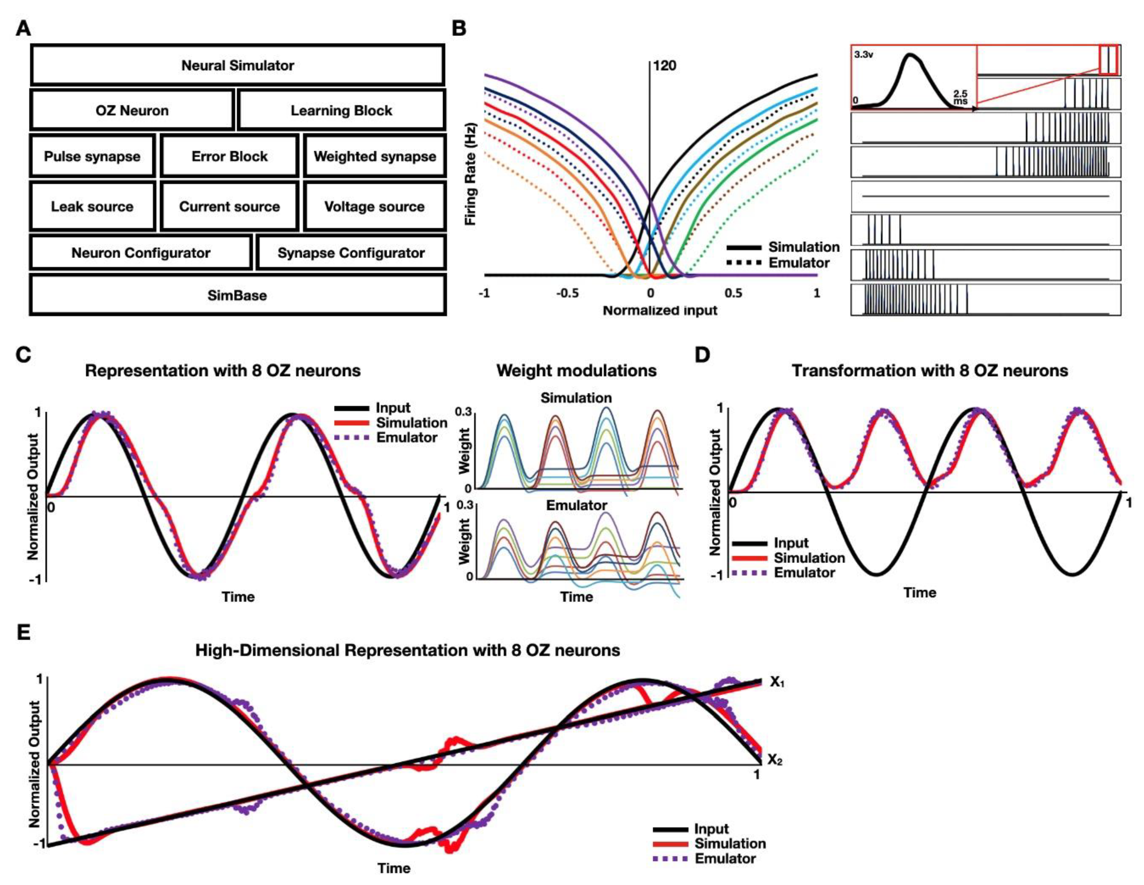
2.6. Circuit Simulation and Emulation
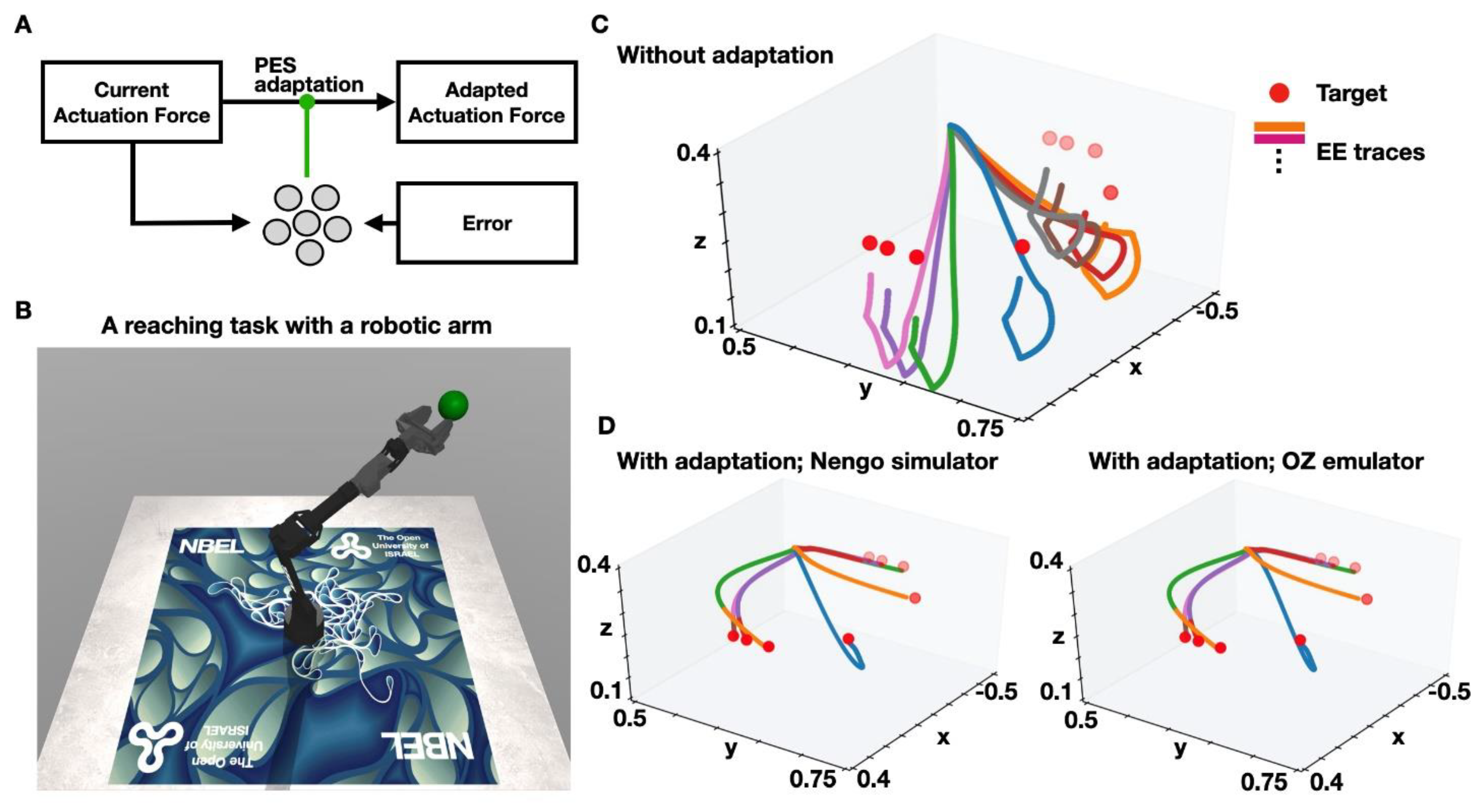
2.7. Robotic Arm Simulation
3. Results
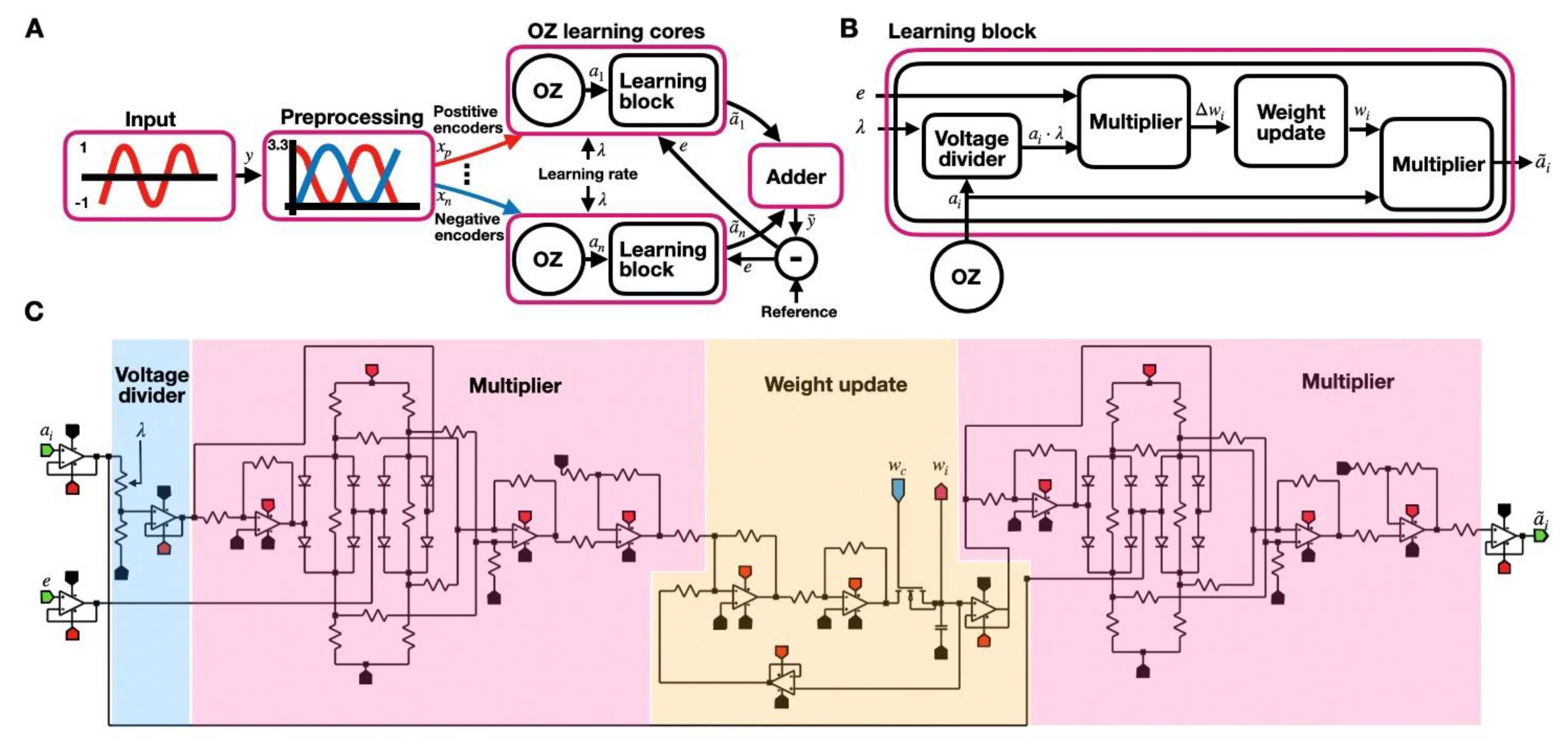
3.1. Circuit Design
3.1.1. Control Circuit
3.1.2. Learning Core
3.2. Circuit Simulation
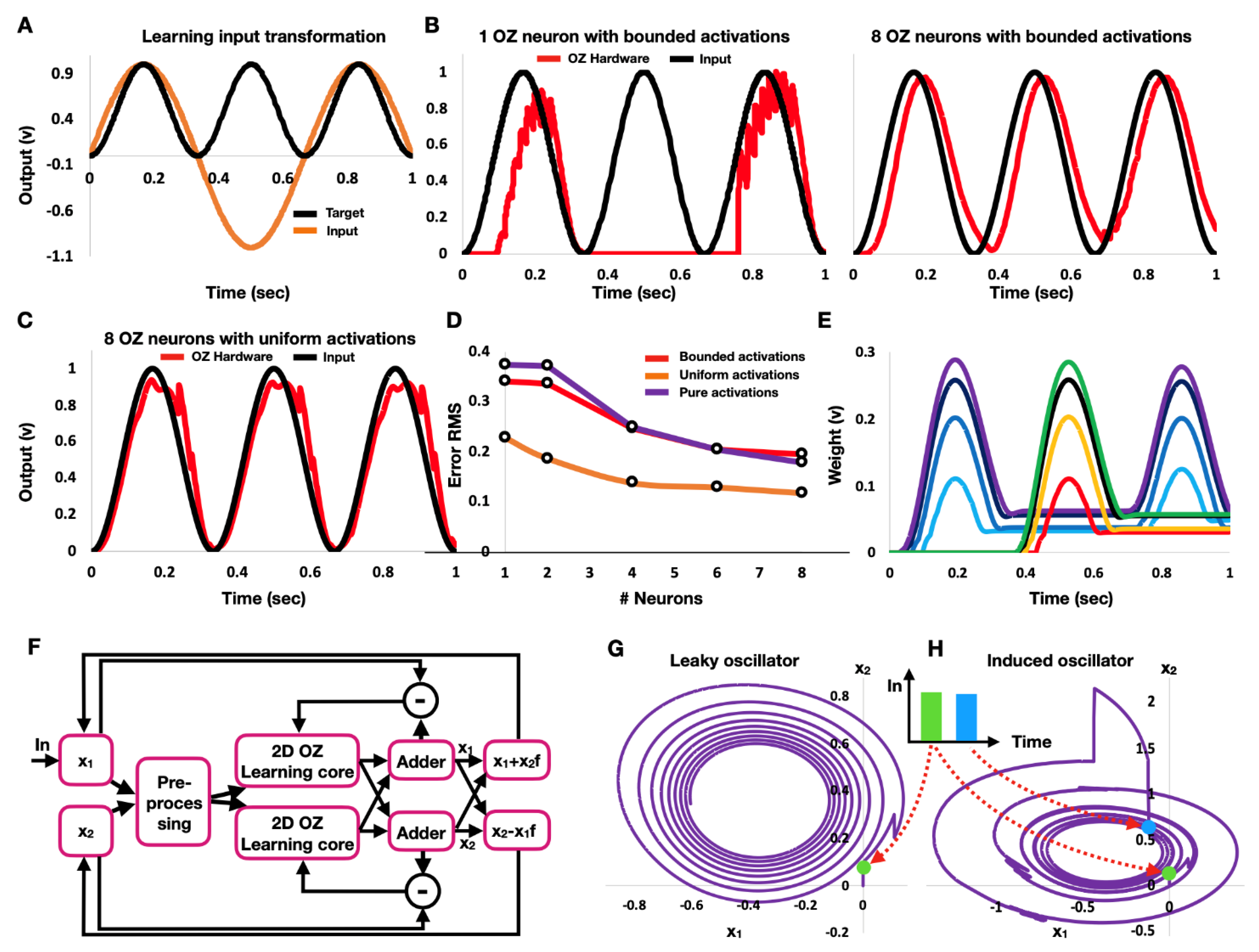
3.2.1. Representation

3.2.2. Transformation
3.2.3. Dynamics
3.2.4. Worst-Case Analysis
3.2.5. Circuit Emulator
3.2.6. Application in Adaptive Neurorobotics
4. Discussion
Author Contributions
Funding
Data Availability Statement
Acknowledgments
Conflicts of Interest
References
- Olkowicz, S.; Kocourek, M.; Lučan, R.K.; Porteš, M.; Fitch, W.T.; Herculano-Houzel, S.; Němec, P. Birds have primate-like numbers of neurons in the forebrain. Proc. Natl. Acad. Sci. USA 2016, 113, 7255–7260. [Google Scholar] [CrossRef] [PubMed] [Green Version]
- Palossi, D.; Loquercio, A.; Conti, F.; Flamand, E.; Scaramuzza, D.; Benini, L. Ultra low power deep-learning-powered autonomous nano drones. In Proceedings of the IEEE/RSJ International Conference on Intelligent Robots and Systems, Madrid, Spain, 1–5 October 2018. [Google Scholar]
- Parisi, G.I.; Kemker, R.; Part, J.L.; Kanan, C.; Wermter, S. Continual lifelong learning with neural networks: A review. Neural Netw. 2019, 113, 54–71. [Google Scholar] [CrossRef] [PubMed]
- Kouvaris, K.; Clune, J.; Kounios, L.; Brede, M.; Watson, R.A. How evolution learns to generalise: Using the principles of learning theory to understand the evolution of developmental organisation. PLoS Comput. Biol. 2017, 13, e1005358. [Google Scholar] [CrossRef] [PubMed]
- Tsur, E.E. Neuromorphic Engineering: The Scientist’s, Algorithm Designer’s, and Computer Architect’s Perspectives on Brain-Inspired Computing; CRC Press: Boca Raton, FL, USA, 2021. [Google Scholar]
- Marković, D.; Mizrahi, A.; Querlioz, D.; Grollier, J. Physics for neuromorphic computing. Nat. Rev. Phys. 2020, 2, 499–510. [Google Scholar] [CrossRef]
- Debole, M.V.; Appuswamy, R.; Carlson, P.J.; Cassidy, A.S.; Datta, P.; Esser, S.K.; Garreau, G.J.; Holland, K.L.; Lekuch, S.; Mastro, M.; et al. TrueNorth: Accelerating From Zero to 64 Million Neurons in 10 Years. Computer 2019, 52, 20–29. [Google Scholar] [CrossRef]
- Davies, M.; Srinivasa, N.; Lin, T.-H.; Chinya, G.; Cao, Y.; Choday, S.H.; Dimou, G.; Joshi, P.; Imam, N.; Jain, S.; et al. Loihi: A Neuromorphic Manycore Processor with On-Chip Learning. IEEE Micro 2018, 38, 82–99. [Google Scholar] [CrossRef]
- Benjamin, B.V.; Gao, P.; McQuinn, E.; Choudhary, S.; Chandrasekaran, A.R.; Bussat, J.-M.; Alvarez-Icaza, R.; Arthur, J.V.; Merolla, P.A.; Boahen, K. Neurogrid: A Mixed-Analog-Digital Multichip System for Large-Scale Neural Simulations. Proc. IEEE 2014, 102, 699–716. [Google Scholar] [CrossRef]
- Furber, S.; Galluppi, F.; Temple, S.; Plana, L.A. The SpiNNaker Project. Proc. IEEE 2014, 102, 652–665. [Google Scholar] [CrossRef]
- Neckar, A.; Fok, S.; Benjamin, B.V.; Stewart, T.C.; Oza, N.N.; Voelker, A.R.; Eliasmith, C.; Manohar, R.; Boahen, K. Braindrop: A Mixed-Signal Neuromorphic Architecture with a Dynamical Systems-Based Programming Model. Proc. IEEE 2018, 107, 144–164. [Google Scholar] [CrossRef]
- Eliasmith, C.; Anderson, C.H. Neural Engineering: Computation, Representation, and Dynamics in Neurobiological Systems; MIT Press: Cambridge, MA, USA, 2004. [Google Scholar]
- Tsur, E.E.; Rivlin-Etzion, M. Neuromorphic implementation of motion detection using oscillation interference. Neurocomputing 2020, 374, 54–63. [Google Scholar] [CrossRef]
- Zaidel, Y.; Shalumov, A.; Volinski, A.; Supic, L.; Tsur, E.E. Neuromorphic NEF-Based Inverse Kinematics and PID Control. Front. Neurorobot. 2021, 15, 631159. [Google Scholar] [CrossRef] [PubMed]
- Hazan, A.; Tsur, E.E. Neuromorphic Analog Implementation of Neural Engineering Framework-Inspired Spiking Neuron for High-Dimensional Representation. Front. Neurosci. 2021, 15, 109. [Google Scholar] [CrossRef] [PubMed]
- Bekolay, T.; Bergstra, J.; Hunsberger, E.; DeWolf, T.; Stewart, T.; Rasmussen, D.; Choo, X.; Voelker, A.; Eliasmith, C. Nengo: A Python tool for building large-scale functional brain models. Front. Neuroinform. 2014, 7, 48. [Google Scholar] [CrossRef] [PubMed]
- Voelker, A.; Kajić, I.; Eliasmith, C. Legendre Memory Units: Continuous-Time Representation in Recurrent Neural Networks. In Proceedings of the 33rd International Conference on Neural Information Processing Systems, Vancouver, BC, Canada, 8–14 December 2019. [Google Scholar]
- Lin, C.-K.; Wild, A.; Chinya, G.N.; Cao, Y.; Davies, M.; Lavery, D.M.; Wang, H. Programming Spiking Neural Networks on Intel’s Loihi. Computer 2018, 51, 52–61. [Google Scholar] [CrossRef]
- Boahen, K. A neuromorph’s prospectus. Comput. Sci. Eng. 2017, 19, 14–28. [Google Scholar] [CrossRef]
- Indiveri, G.; Douglas, R. Neuromorphic Vision Sensors. Science 2000, 288, 1189–1190. [Google Scholar] [CrossRef]
- Liu, S.-C.; Delbruck, T. Neuromorphic sensory systems. Curr. Opin. Neurobiol. 2010, 20, 288–295. [Google Scholar] [CrossRef]
- Voelker, A.R. A Solution to the Dynamics of the Prescribed Error Sensitivity Learning Rule; Centre for Theoretical Neuroscience: Waterloo, ON, Canada, 2015. [Google Scholar]
- Devices, A. LTspice Simulator. 2008. Available online: http://www.analog.com/en/design-center/design-tools-and-calculators/ltspice-simulator.html (accessed on 26 September 2020).
- Nagel, L.; Pederson, D. SPICE (Simulation Program with Integrated Circuit Emphasis); University of California: Berkeley, CA, USA, 1973. [Google Scholar]
- Nichols, K.; Kazmierski, T.; Zwolinski, M.; Brown, A. Overview of SPICE-like circuit simulation algorithms. IEE Proc. Circuits Devices Syst. 1994, 141, 242–250. [Google Scholar] [CrossRef]
- Mittal, S. A Survey of Architectural Techniques for Managing Process Variation. ACM Comput. Surv. 2016, 48, 1–29. [Google Scholar] [CrossRef]
- Lanfranco, A.R.; Castellanos, A.E.; Desai, J.P.; Meyers, W.C. Robotic surgery: A current perspective. Ann. Surg. 2004, 239, 14. [Google Scholar] [CrossRef]
- Nishida, S.-I.; Kawamoto, S.; Okawa, Y.; Terui, F.; Kitamura, S. Space Debris Removal System using a Small Satellite. Acta Astronaut. 2009, 65, 95–102. [Google Scholar] [CrossRef]
- DeWolf, T.; Stewart, T.C.; Slotine, J.-J.; Eliasmith, C. A spiking neural model of adaptive arm control. Proc. R. Soc. B Boil. Sci. 2016, 283, 20162134. [Google Scholar] [CrossRef] [PubMed] [Green Version]
- Eliasmith, C. How to Build a Brain: A Neural Architecture for Biological Cognition; Oxford University Press: Oxford, UK, 2013. [Google Scholar]
- Applied Brain Research Inc. Available online: https://www.nengo.ai/nengo-loihi/v0.9.0/examples/learn_communication_channel.html (accessed on 26 March 2021).
- Fischl, K.D.; Andreou, A.G.; Stewart, T.C.; Fair, K. Implementation of the Neural Engineering Framework on the TrueNorth Neurosynaptic System. In Proceedings of the 2018 IEEE Biomedical Circuits and Systems Conference (BioCAS), Cleveland, OH, USA, 17–19 October 2018. [Google Scholar]
- Mundy, A.; Knight, J.; Stewart, T.C.; Furber, S. An efficient SpiNNaker implementation of the Neural Engineering Framework. In Proceedings of the 2015 International Joint Conference on Neural Networks (IJCNN), Killarney, Ireland, 12–16 July 2015. [Google Scholar]


Publisher’s Note: MDPI stays neutral with regard to jurisdictional claims in published maps and institutional affiliations. |
© 2022 by the authors. Licensee MDPI, Basel, Switzerland. This article is an open access article distributed under the terms and conditions of the Creative Commons Attribution (CC BY) license (https://creativecommons.org/licenses/by/4.0/).
Share and Cite
Hazan, A.; Ezra Tsur, E. Neuromorphic Neural Engineering Framework-Inspired Online Continuous Learning with Analog Circuitry. Appl. Sci. 2022, 12, 4528. https://doi.org/10.3390/app12094528
Hazan A, Ezra Tsur E. Neuromorphic Neural Engineering Framework-Inspired Online Continuous Learning with Analog Circuitry. Applied Sciences. 2022; 12(9):4528. https://doi.org/10.3390/app12094528
Chicago/Turabian StyleHazan, Avi, and Elishai Ezra Tsur. 2022. "Neuromorphic Neural Engineering Framework-Inspired Online Continuous Learning with Analog Circuitry" Applied Sciences 12, no. 9: 4528. https://doi.org/10.3390/app12094528
APA StyleHazan, A., & Ezra Tsur, E. (2022). Neuromorphic Neural Engineering Framework-Inspired Online Continuous Learning with Analog Circuitry. Applied Sciences, 12(9), 4528. https://doi.org/10.3390/app12094528