Hydro-Mechanically Coupled Numerical Modelling on Vibratory Open-Ended Pile Driving in Saturated Sand

Abstract

Vibratory pile diving with resonance-free technique is an advanced construction approach that can play an important part in underground engineering. This paper aims to propose a numerical model for this construction approach, which commonly involves soils below the groundwater table. Such simulations are still challenging tasks as dynamic analyses considering hydro-mechanical interactions are very complicated. Several simulations have been performed by constructing a user-defined element in the finite element code ABAQUS or developing an inhouse finite-element program for this issue. These simulations have some limitations and pay less attention to open-ended piles. This paper presents a way to simulate the vibratory open-ended pile driving in saturated sand using the finite difference code FLAC3D. The model computation efficiency is increased around 67 times by the density scaling method and this method has little effect on the numerical stability. The proposed model can generally replicate the pore pressure results of a model test. The maximum excess pore pressures are predicted with a percent error of 2–22%, and these maximums occur near the pile toe. The excess pore pressure of an observation point slowly decreases after the pile toe passes the point. This work could provide an efficient and effective method for simulating vibratory open-ended pile driving in saturated sand.

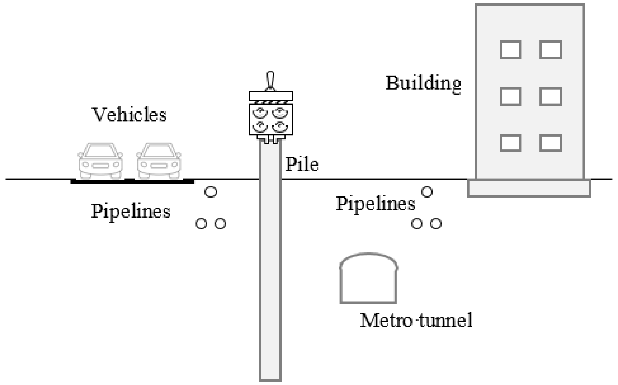
1. Introduction

Vibratory pile driving is a pile installation technique that exploits the continuous periodic load from a vibratory hammer as a driving force. Along with the evolution of the vibratory hammer, a vibratory pile driving with resonance technique springs up in urban areas mainly because this construction approach has advantages in terms of the pile installation speed and the environmental impact [1,2,3,4]. As reported in [4], the driving time for an open-ended steel pile (pile diameter 700 mm and pile length 60 m) is less than 40 min, and the maximum ground surface vibration measured at around 1 m from the pile axis is as low as 13.32 mm/s. The terminology of resonance-free means that the severe vibration influences caused by the resonance phenomenon can be mitigated and avoided during pile installation. The principle of resonance-free technique is that the novel vibratory hammer has a high work frequency as well as generating zero centrifugal force during start-up and shut-down [4,5,6].

The advantages of vibratory pile driving with resonance-free technique can contribute to underground constructions that often require a short construction period or encounter a complicated construction environment (Figure 1). To better exploit this novel construction approach, more investigations are still needed. Numerical simulation is a cost-effective method. According to the principle of resonance-free [4,5,6] technique, the simulation of resonance-free vibratory pile driving can be treated as conventional vibratory pile driving if the start-up and shut-down processes are able to be neglected.

As vibratory pile driving commonly involves soils below the groundwater table, it is critical to consider the hydro-mechanical interactions in numerical studies. However, considering hydro-mechanical interactions in the dynamic analysis is particularly difficult when dealing with the vibratory penetration problem. Most simulations of vibratory pile driving take simplified assumptions for the hydro-mechanical interactions. These assumptions vary from dry condition [7,8,9], undrained condition [6,10,11], to locally undrained condition (zero soil permeability) [12,13]. Additionally, although some simulations modelling vibratory pile driving under a partly drained condition (nonzero soil permeability) have been reported, the simulated pile penetrations were zero [14], or very small [15].

To the authors’ knowledge, a few simulations have incorporated both the partly drained condition and substantial pile penetration [16,17,18,19]. Certain efforts were made to construct a user-defined element for the dynamic analysis of hydro-mechanical interactions when these simulations were performed in the finite element code ABAQUS. Machacek et al. [18] and Staubach et al. [19] also carried out several simulations using an inhouse finite-element program NUMGEO, which they developed. Unfortunately, the pile–soil contact might be poorly modelled using ABAQUS as implementations of pile–soil contact were either restricted to a frictionless contact [16,17] or incapable of calculating the effective contact pressure [19]. Simulations performed using NUMGEO [18,19] are able to incorporate both frictional contact and effective contact pressure. However, NUMGEO is still under development and not yet available to the public [20]. Moreover, the reviewed studies mainly focused on close-ended piles [16,17,18,19], rarely involving open-ended piles, which are popular in practice [1,2,3,4]. Overall, the simulation of vibratory pile driving in saturated soil is still challenging task.

The authors of this paper have been working on modelling vibratory pile driving using the finite difference software FLAC3D [6,11]. There is a build-in procedure available for dynamic analysis of hydro-mechanical interactions in FLAC3D [21]. A numerical model is established in this paper for vibratory open-ended pile driving in saturated sand using FLAC3D. A density scaling method is used to increase the computation efficiency of the proposed model. The pile motion characteristic is analyzed according to the numerical results. The pore pressure responses from published experimental results are used as validation sources to test the proposed model. The simulated pore pressure results are also analyzed from the aspects of evolution and distribution.

The structure of this paper is as follows. In Section 2, a brief description of a published experiment on vibratory pile driving [8] is presented. Section 3 presents the establishment of the numerical model in FLAC3D. Section 4 shows the influence of the density scaling method on numerical stability. In Section 5, the results of the proposed model are validated and discussed. In Section 6, value differences between the numerical results and the measured values [8] are discussed. The conclusion is presented in Section 7.

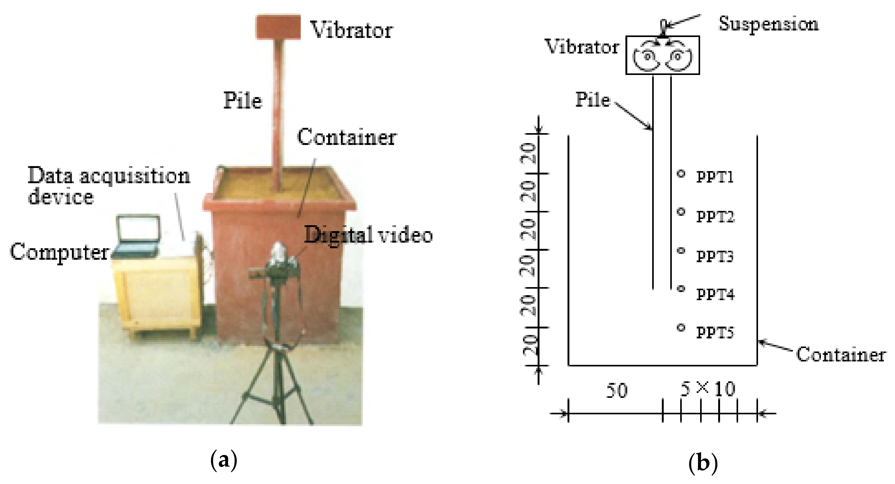
2. Brief Description of the Vibratory Pile Driving Experiment

Experimental data are often exploited to establish and validate models in numerical studies. There are a few vibratory pile driving experiments available. These experiments may be roughly divided into two categories: (a) experiment of the open-ended pile [8,22], and (b) experiment of the close-ended pile [23,24]. Considering the great popularity of vibratory open-ended pile driving in practice [1,2,3,4], the experiment conducted by Xiao et al. [8] was reproduced using the numerical model in this paper. As shown in Figure 2a, the experiment was a three-dimensional model test, in which an open-ended pile was penetrated into water-saturated sand by a vibrator, and the pore pressure near the pile axis was recorded during vibratory penetration.

The size of the experiment container was 100 cm long, 100 cm wide, and 120 cm high. The saturated sand specimen was made of Fujian sand (a kind of fine quartz sand). The saturated density $\rho$ and the internal friction angle $\phi$ of the specimen were 1924 kg/m³ and 28°, respectively. An open-ended steel pile with a diameter of D = 5.0 cm, wall thickness of 0.3 cm, and length of 150.0 cm was used in the experiment. Figure 2b shows the guideless vibrator on the pile head (the support device is not shown in [8]). The vibrator could provide a periodic load with a frequency of 20 Hz on the pile head. As presented in Figure 2b, there were five pore pressure transducers (PPT) at the same radial distance R = 2D from the pile axis. The type of PPTs was a resistance strain sensor. Their buried depths H were 4D, 8D, 12D, 16D, and 20D, respectively. The vibratory penetration began from the specimen surface and ended at a depth of 16D.

3. Numerical Model

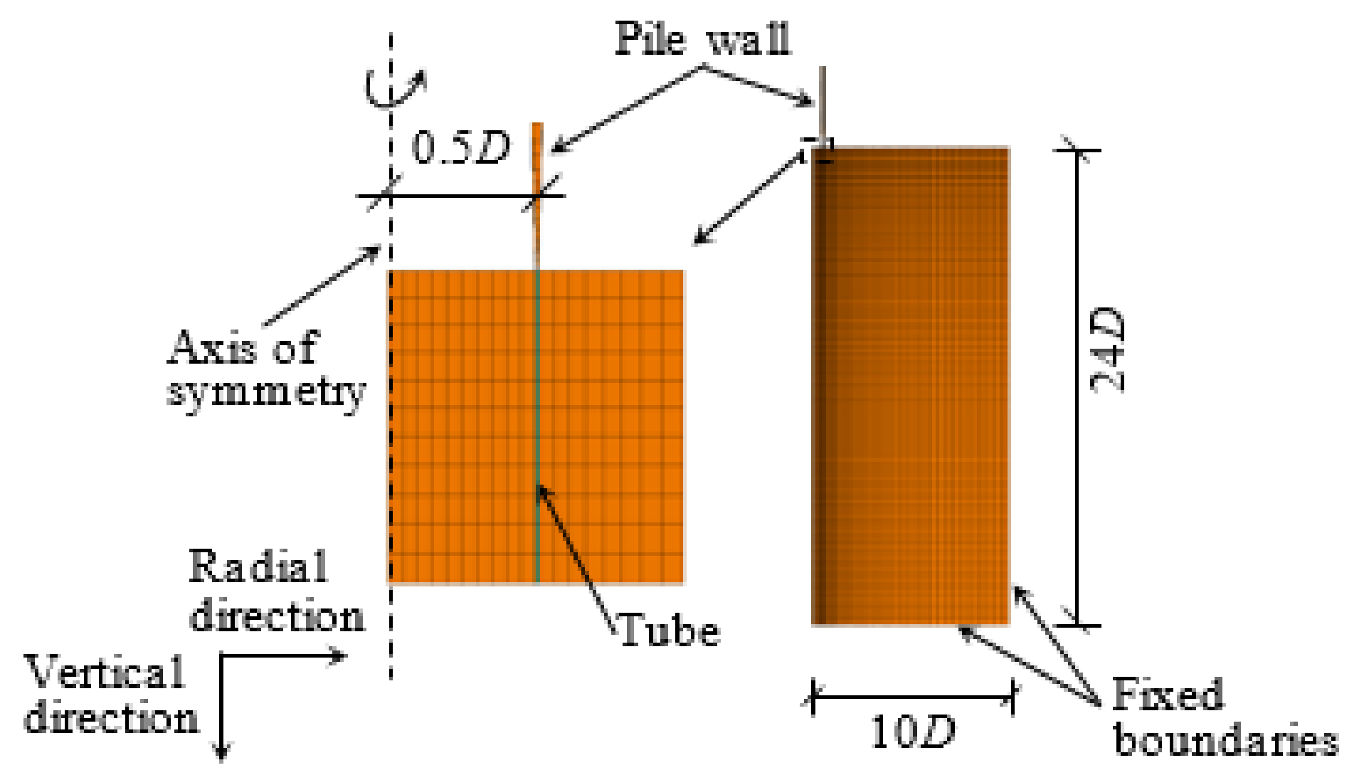
3.1. Geometry Model

Vibratory open-ended pile driving can be treated as an axisymmetric problem. Figure 3 presents an axisymmetric model to reproduce the experiment mentioned above. The radial and vertical sizes of the soil model are 10D and 24D, respectively.

A zipper-type technique, which has been exploited to simulate vibratory open-ended pile driving [6,7,11], is adopted in this paper to incorporate the formation of pile–soil contact. According to the zipper-type technique, a fictitious and frictionless rigid tube is embedded in the soil beforehand, as depicted in Figure 3. The tube thickness is 0.03 cm, one-tenth of the pile wall thickness. When the pile penetrates the soil, the pile wall slides along the fixed tube, and the soil is separated from the tube, establishing a pile–soil contact.

In numerical analyses, finer mesh resolution often results in accuracy improvement of the numerical solution, but always accompanies with a higher computation burden. It is therefore important to choose a suitable grid density, especially for dynamic numerical analyses. In order to better model the pile–soil interaction, the mesh of soil elements was refined near the pile shaft. The smallest size of soil elements is around 0.25 cm, about one-tenth of the pile diameter. The whole model has 9420 elements and 20,406 grid points, whose mesh diagram is shown in Figure 3.

As for boundary conditions, the right and bottom boundaries were all fixed, as they were in the experiment. The pore pressure was set to zero at the top surface, and other boundaries were defined as impermeable. Particularly, the large-strain mode in FLAC3D was used to mitigate the probable mesh distortion. In the large-strain mode, node coordinates were updated, and stress rotation was corrected [21].

3.2. Material Parameters

To take into account the generation of dynamic pore pressure, the Finn model in FLAC3D was chosen as the soil constitutive model. The Finn model contains two optional formulations: the Martin et al. formulation and the Byrne formulation. The Byrne formulation is a modified and simplified formula based on the Martin et al. formulation [21] and was adopted in this paper. The applied soil parameters are shown in

Table 1. Material parameters in the numerical model.

Material	Constitutive Model	Density $\mathit{\rho }$ [kg/m3]	Elastic Modulus E [GPa]	Poisson’s Ratio $\mathit{\upsilon }$	Internal Friction Angle $\mathit{\phi }$ [°]	N1 *
Sand	Finn	1924	0.02	0.28	28	6
Pile	Elastic	7850	206	0.26
Tube	Elastic	7850	206	0.26

* N₁ is the normalized standard penetration test value.

. To simulate the material damping, a local damping ratio of 20% was used during vibratory penetration.

A hydro-mechanically coupled model requires many parameters, including the void ratio, the hydraulic conductivity, and the fluid bulk modulus, which were not reported in their experiment [8], unfortunately. In this paper, the void ratio and the hydraulic conductivity were assigned as 0.72 and 5 × 10⁻³ cm/s, respectively. As shown in Figure 2, the fully saturated condition is actually hard to assure. Thus, the sand saturation was assumed to be 99%, approximately corresponding to a fluid bulk modulus of 20 MPa [12,13].

In other studies of vibratory pile driving [7,8,9,10,12,13,14,15,16,17,18,19], piles are often regarded as rigid piles. However, when piles and tubes are composed of zone elements in FLAC3D, rigidity is not applicable for piles and tubes. The elastic model is thus applied for the pile and the tube, and the related parameter is shown in Table 1.

3.3. Contact Parameters

In FLAC3D, the soil–structure contact can be modelled by interface elements, which are defined using three nodes (interface nodes). When another grid surface comes into contact with an interface element, the contact can be detected at the interface node. At each time step, the absolute normal penetration and the relative shear velocity are solved at each interface node and transferred to the contacting target face. Then, the normal force and the shear force are correspondingly calculated. More details about the interface element can be seen in the user’s guide manual of FLAC3D [21].

The Coulomb friction model was used as the contact constitutive model in this paper. The normal stiffness and shear stiffness were obtained by trial and error analysis. The pile–soil friction angle of 10° was applied according to the literature [6,7,11]. The tube–soil friction angle was set to 0°, representing the frictionless tube. Note that the calculation mode of effective contact stress was also adopted in the simulations, and the contact parameters used in the analysis are given in

Table 2. Contact parameters in the numerical model.

Type	Normal Stiffness kn [GPa·m]	Shear Stiffness ks [GPa·m]	Friction Angle $\mathit{\delta }$ [°]
Pile–soil	0.2	0.2	10
Tube–soil	8	8	0

.

3.4. Load Parameters

As described in the following Equations (1) and (2), during vibratory pile driving, the force on the pile $F_{\mathrm{p}}$ can be divided into three parts: (a) the vibrating force $F_{\mathrm{v}}$ developed by a set of counter-rotating eccentric mass in a vibrator, (b) the static force $F_{\mathrm{s}}$, which is the resultant force of supporting force and pile-vibrator deadweight, and (c) the resistance of pile penetration $F_{\mathrm{r}}$, which is the reaction force from the soil.

$$F_{\mathrm{p}}=F_{\mathrm{v}}+F_{\mathrm{s}}+F_{\mathrm{r}}$$

(1)

$$F_{\mathrm{v}}=F_{\mathrm{vm}}\sin \left(2\mathsf{\pi }ft\right)$$

(2)

where $F_{\mathrm{vm}}$ is the vibrating force amplitude, $f$ is the vibrator frequency, and $t$ is the driving time.

The vibrator frequency $f$ was 20 Hz, which is in line with the experiment. $F_{\mathrm{vm}}$ and $F_{\mathrm{s}}$ were assigned as 4.0 G and 0.2 G, respectively, where the pile deadweight G was 34.5 N in this paper. The penetration resistance $F_{\mathrm{r}}$ was updated by summing up the pile–soil contact force during pile penetration.

The dynamic analysis in FLAC3D is based on an explicit finite difference scheme, in which the model is solved numerically using an explicit finite difference formulation in time. The maximum stable time increment $∆t_m$ is calculated by Equations (3) and (4) [21]:

$$∆t_m=0.5min\left(\frac{V}{C_p{A}_{max}^f}\right)$$

(3)

$$C_p=\sqrt{\frac{E\left(1-\upsilon \right)}{\rho \left(1-2\upsilon \right)\left(1+\upsilon \right)}}$$

(4)

where $C_p$ is the compression wave speed, $V$ is the tetrahedral subzone volume, $A_{max}^f$ is the maximum face area associated with the tetrahedral subzone, the min ( ) function is applied to all zones.

A smaller $∆t_m$ brings more computation time. In this paper, the original $∆t_m$ was around 1.6 × 10⁻⁸ s due to the excessive elastic modulus (206 Gpa) of the pile and the tube. In order to decrease the time cost, the density scaling method [6,11] was used. In this method, referring to Equations (3) and (4), densities of the pile and the tube were scaled down to increase $∆t_m$, and the $F_{\mathrm{p}}$ was also enlarged by the same scale to avoid the abnormal acceleration, see Equation (5) [6]. The alternative to decrease computation time is a mass scaling method, which can be used in finite element software like ABAQUS [25]. The difference between the two methods is that the pile acceleration will remain normal by enlarging the $F_{\mathrm{p}}$ in the density scaling method.

$$a_{\mathrm{p}}=\frac{ng{F}_{\mathrm{p}}}{nG}$$

(5)

where n is the scaling factor, $g$ is the gravity acceleration of 10 m/s².

To determine the scaling factor (SF), a series of SF were tested. Figure 4 presents the relation between the SF and the $∆t_m$. It is clear that the $∆t_m$ stops increasing when the SF is greater than 10⁵. In the present study, SF = 10⁶ was applied, and correspondingly the $∆t_m$ was 3.1 × 10⁻⁶ s.

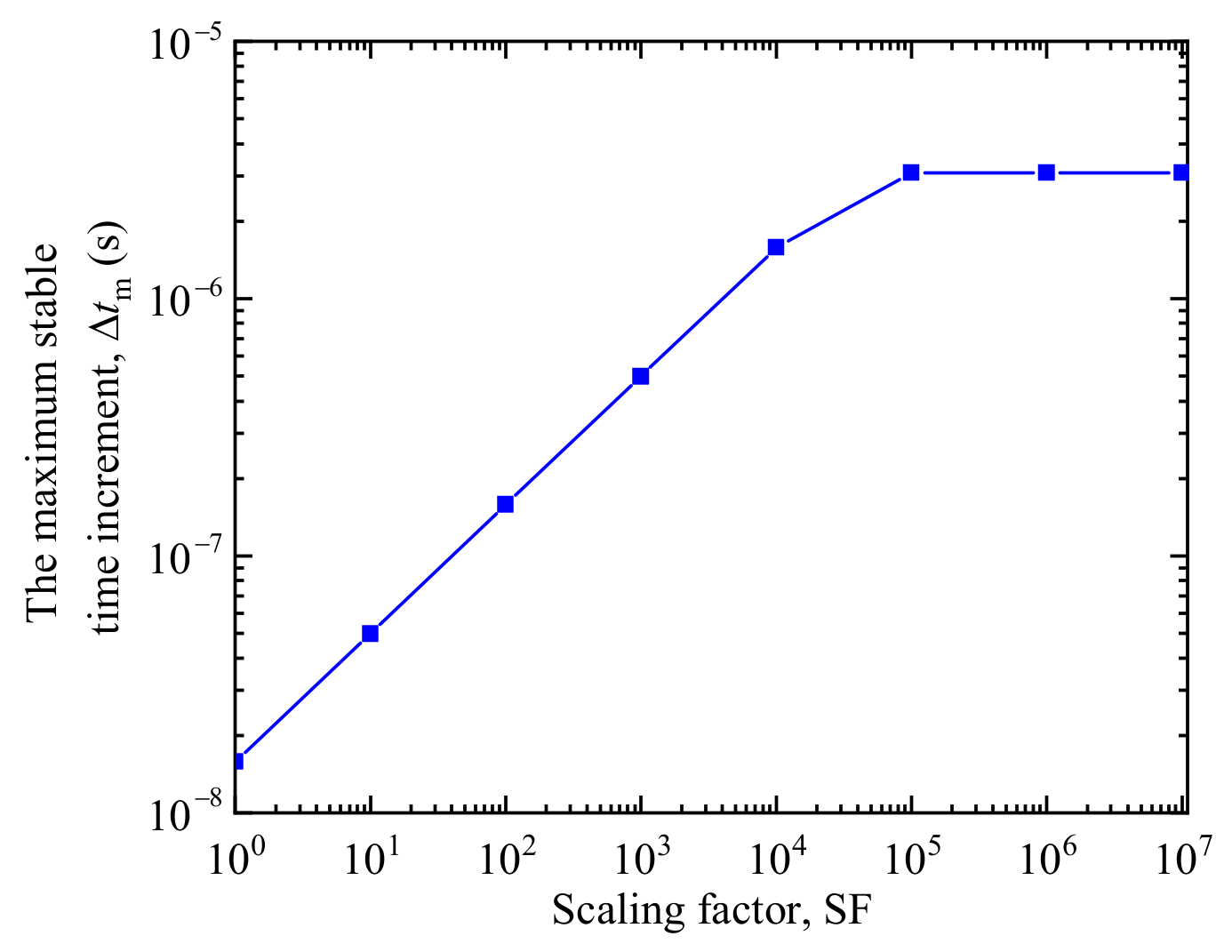
4. Influence of the Scaling Factor

In order to study the influence of SF on the numerical result, a case without using the density scaling method (i.e., SF = 1) was performed by the same high-performance computer. The computation time of the two cases was firstly compared. It took about 140.0 h for SF = 1 when the penetration depth reached 8D. Remarkably, it took only about 2.1 h for SF = 10⁶ when the pile arrived at the same depth, proving the scaling factor has a significant impact on the computation time. The computation efficiency is increased approximately 67 times.

Figure 5 compares the vertical distribution of excess pore pressure $∆p$ for SF = 1 and SF = 10⁶. One can see a slight difference that only occurs when the penetration depth L is 4D. Thus, it is feasible to believe that the scaling factor has little effect on the $∆p$, and the density scaling method [6,11] can increase the computation efficiency of the proposed model without decreasing accuracy.

5. Results of the Proposed Model

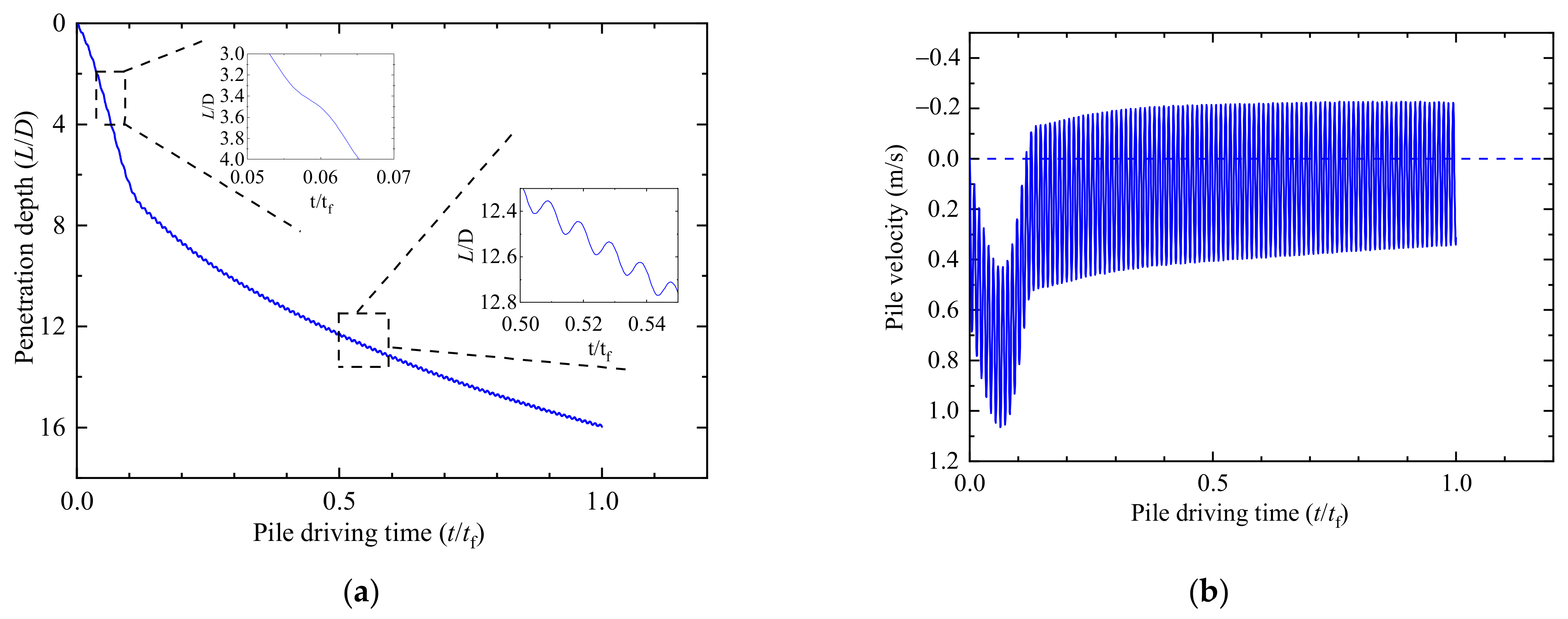
5.1. Pile Displacement and Velocity

During vibratory penetration, the pile toe penetrated the soil from the surface and stopped at the penetration depth of 16D. Time histories of the penetration depth (L) and pile velocity are plotted in Figure 6a,b, respectively, where the driving time t is normalized by the completion time t_f.

As shown in Figure 6a, the time history of the pile displacement can be divided into two distinct stages. In the first stage, the pile penetrates downward stably, and the corresponding velocities remain positive from Figure 6b. The monotonic penetration mode can be attributed to little penetration resistance compared with the driving force at the shallow layer. In the second stage, the pile displacement oscillates continuously. From Figure 6b, the corresponding velocity direction is averagely downward, but fluctuates upward frequently. The oscillation is caused by more significant penetration resistance at the deep layer. In general, the proposed model has captured the motion characteristic of vibratory penetration.

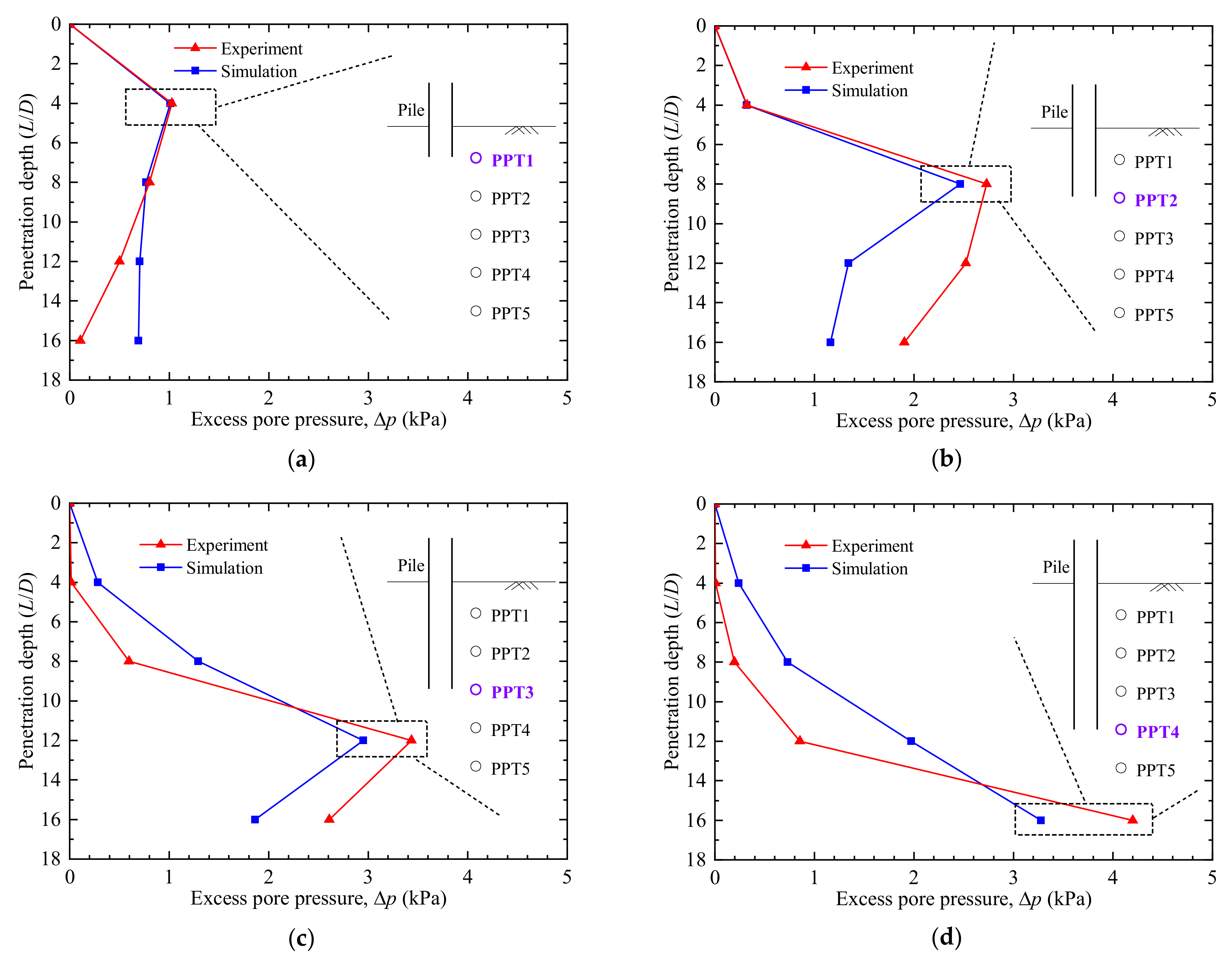
5.2. Comparison between Numerical and Experimental Results

To validate the proposed model, this paper focuses on whether the numerical model can reproduce the pore pressure response measured in [8]. The simulated correlation between excess pore pressure $∆p$ and the increase of penetration depth is compared with the tested result, see Figure 7a–d for the comparisons of PPT1~PPT4, respectively.

All curves in Figure 7a–c show that $∆p$ keeps increasing until the penetration depth reaches the depth of the observation point, and then gradually decreases. In this $∆p$ trend, there is a good agreement between the tested and simulated results. Furthermore, this trend has been observed in studies of vibratory close-ended pile driving [16,17,19,24]. Note that the $∆p$ in Figure 7d continuously increases throughout the penetration process because the pile toe did not pass by PPT4.

From Figure 7a–c, one can also notice that both the experiment and the simulation indicate that the maximum $∆p$ of different observation points is related to their depths. Specifically, the maximum $∆p$ increases with the depth of the observation point. This may be attributed to the increase of penetration resistance in the deeper soil. Large penetration resistance reduces the pile velocity, and thus the observation point is subjected to more vibrations, resulting in the increase of $∆p$. A similar trend can also be found in the literature [16,24], in which a more significant response of pore pressure occurs at a deeper point.

Figure 8 compares the distribution of $∆p$ at different penetration depths L between experiment and simulation. Three key points can be seen in Figure 8. Firstly, all the maximum $∆p$ occur near the pile toe. For example, the maximum $∆p$ at L = 8D occurs at the buried depth of 8D. Secondly, for a certain penetration depth, $∆p$ increases with the buried depth when the observation point is above the pile toe and decreases with the buried depth when the observation point is below the pile toe. Finally, the maximum $∆p$ at different L rises as the depth of pile toe increases. Generally, the proposed model is capable of capturing the essential aspects of the experiment result in terms of $∆p$ distribution.

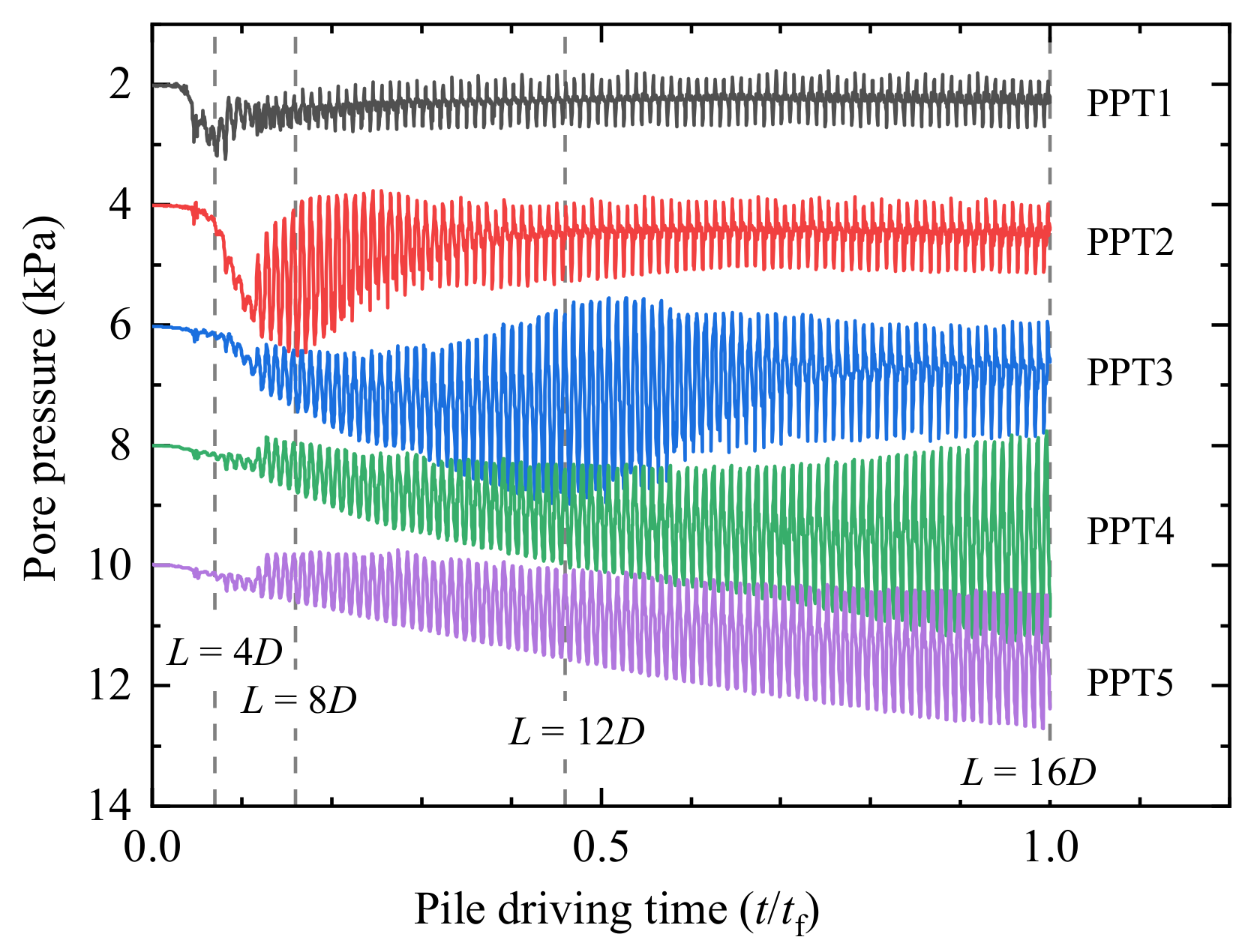
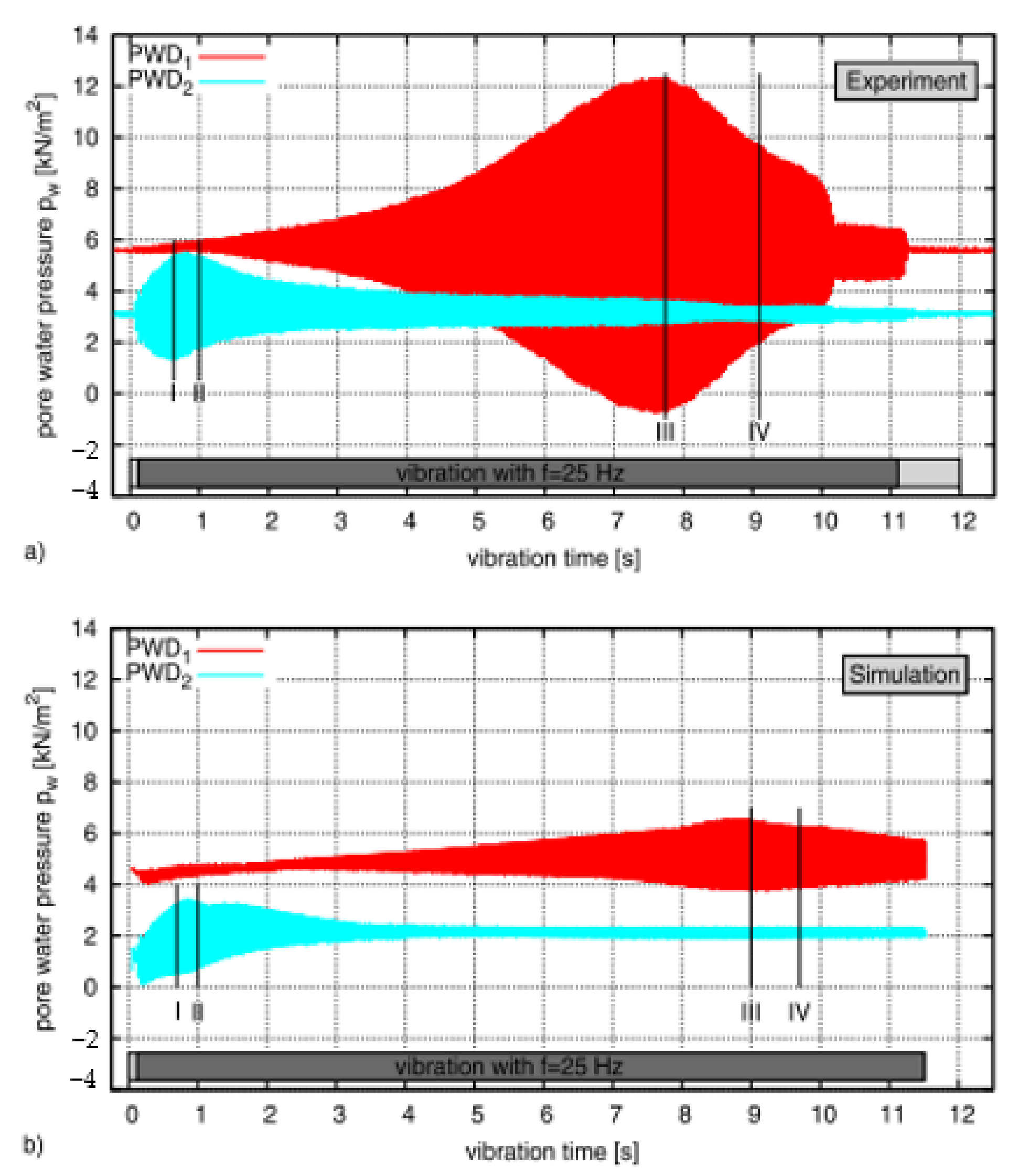
5.3. Evolution of Pore Pressure

The simulated time history of pore pressure is shown in Figure 9, whereas the corresponding experimental data are not available. Three obvious peak amplitudes can be seen for PPT1, PPT2, and PPT3 when the pile toe passes by the observation point. This phenomenon has also been reported in other studies [16,17,19,24]. Field test data of Moriyasu et al. [22] showed that if the pore pressure was measured near the pile shaft, the peak value would be reached before the pile toe passes. The reported peak response may need further investigation because only one pore pressure transducer was used, and there were five different pile installations. As for PPT4 and PPT5, the amplitudes increase monotonously as the pile toe does not pass them. Finally, a slight increase in the overall trend of the pore pressure development can be observed for PPT1, PPT2, and PPT3, and this increase is more evident for PPT4 and PPT5.

In soil dynamic analyses, with vibration time increasing, the excess pore pressure accumulates before the soil liquefaction. As shown in Figure 9, however, the pore pressure does not keep accumulating along with the pile driving time after the pile toe reaches the depth of the observation point. The possibility of the soil liquefaction can be excluded as the pore pressure falls off rather than remains at a stable value. As reported in Chrisopolous et al. [16] and Moriyasu et al. [22], liquefaction-like phenomena also do not appear in vibratory pile driving. The pore pressure evolution can be paid more attention to better understand the penetrating mechanism of vibratory driven piles.

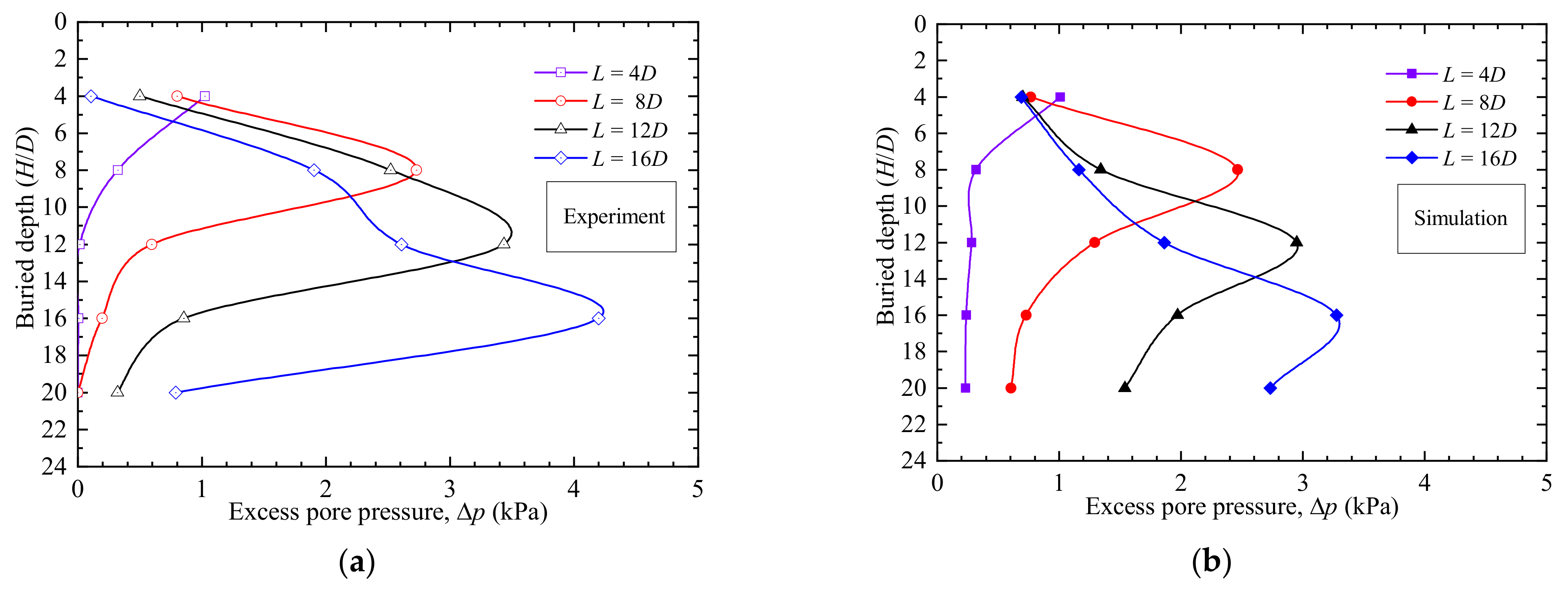
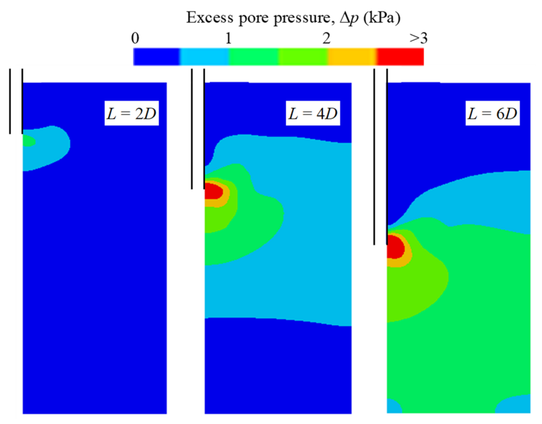
5.4. Field Distribution of Excess Pore Pressure

Field distributions of excess pore pressure $∆p$ at different penetration depths L are displayed in Figure 10. It is apparent that the maximum $∆p$ occurs in the vicinity of the pile toe. With the increase of penetration depth, the influence range of $∆p$ enlarges. From Figure 10, the influence range of $∆p$ gradually exceeds the model domain during vibratory pile driving. In the vertical direction, the influenced area goes beyond the lower extent of the soil model when L = 6D. For the influence radius, it begins to exceed the radial size of the soil model when L = 4D.

6. Discussion

It can be seen that the proposed model is able to reproduce the pore pressure development in a qualitative manner, but shows some discrepancies compared with the experiment data. During vibratory pile driving, the maximum excess pore pressure is usually one of the key indices to predict the construction influence in geotechnical engineering. In Figure 8, the percent error of 2–22% can be seen when the maximum excess pore pressure recorded at different penetration depths are compared between the simulation and the experiment. This error range could be accepted in most geotechnical engineering practices. It should also be pointed out that value differences between simulations and experiments can also be found in the literature [16,17,18,19]. For example in the literature [16], there are significant discrepancies of maximum excess pore pressure between the simulation and the experiment (Figure 11). In Figure 11, the approximate errors are 68% for the PWD1 and 4% for the PWD2, respectively. Compared with the results in Figure 11, the proposed model seems to have a better ability to predict the maximum excess pore pressure from the measurement.

In the presented paper, the underlying reasons for the discrepancies between the simulation and the experiment may include two points. Firstly, there are fixed boundary conditions with small model sizes both in the experiment and the simulation. The reflection of waves at boundaries can make the measured values difficult to be replicated in the simulation. Secondly, as reported in [16], the soil mechanical characteristics are complicated to be modelled by most soil constitutive models during vibratory penetration. For example, there are large numbers of load or deformation cycles on the soil. Furthermore, the large monotonic deformation and the cyclic deformation concurrently exist on the vibratory pile penetration.

7. Conclusions

Numerical studies of vibratory pile driving with resonance-free technique can facilitate the use of this novel construction approach in underground engineering. In this paper, a hydro-mechanically coupled model is proposed for vibratory open-ended pile driving in saturated sand using FLAC3D. The main conclusions are as follows.

• The scaling factor has a significant impact on the computation time but has little effect on the distribution of excess pore water pressure $∆p$. The computation efficiency of the proposed model is increased around 67 times by the density scaling method without affecting the numerical stability.
• The results from the proposed model are reliable because (a) the trends of measured pore pressures can be reproduced, and (b) the measured maximum $∆p$ at different depths can be predicted with a percent error of 2–22%.
• For a certain penetration depth, the $∆p$ increases and then decreases in the vertical direction as the observation points are 2D away from the pile axis. The maximum $∆p$ occurs near the pile toe. For a specified observation point, its $∆p$ reaches the maximum when the pile toe passes the point and gradually decreases afterwards. The influence scope of $∆p$ enlarge along with the vibratory penetration.

More researchers may work on the simulation of vibratory pile driving with resonance-free technique due to its advantages in practice. The proposed model provides a reference for this topic. We do not take the proposed numerical model as the end of the story. A sophisticated experiment of vibratory open-ended pile driving will be performed to record time histories of pore pressure.

References

- Yang, C.L. Experimental study on vibration effect of steel pipe piles resonance-free construction on adjacent metro. Build. Struct. 2018, 40, 1655–1657. (In Chinese) [Google Scholar] [CrossRef]
- Li, C.; Zhang, M.X.; Zhou, R.F.; Wang, Z.Q. In-situ test on resonance-free pile. J. Yangtze River Sci. Res. Inst. 2020, 37, 122–127. (In Chinese) [Google Scholar] [CrossRef]
- Arjen. Indoor Piling Job at NECC. Available online: https://www.icevibro.com/article/406/8.html (accessed on 17 July 2019).
- Wang, W.D.; Wei, J.B.; Wu, J.B.; Zhou, R.F. Field test and analysis on effects of pile driving with high-frequency and resonance-free technology on surrounding soil. J. Build. Struct. 2021, 42, 131–138. (In Chinese) [Google Scholar] [CrossRef]
- International Construction Equipment (ICE). Resonance Free Vibratory Hammers. Available online: https://www.diesekogroup.com/landing-page/resonance-free/ (accessed on 4 October 2021).
- Wei, J.B.; Wang, W.D.; Wu, J.B. Numerical investigation of inside peak particle velocities for predicting the vibration influence radius of vibratory pile driving. Soil Dyn. Earthq. Eng. 2022, 153, 107103. [Google Scholar] [CrossRef]
- Henke, S.; Grabe, J. Numerical investigation of soil plugging inside open-ended piles with respect to the installation method. Acta Geotech. 2008, 3, 215–223. [Google Scholar] [CrossRef]
- Xiao, Y.J.; Chen, F.Q.; Dong, Y.Z. Model test and numerical simulation of penetration process of sleeve for cast-in-place piles driven by vibratory hammers. J. Southwest Jiaotong Univ. 2017, 52, 705–714. (In Chinese) [Google Scholar] [CrossRef]
- Wang, S.G.; Zhu, S.Y. Global Vibration Intensity Assessment Based on Vibration Source Localization on Construction Sites: Application to Vibratory Sheet Piling. Appl. Sci. 2022, 12, 1946. [Google Scholar] [CrossRef]
- Ekanayake, S.D.; Liyanapathirana, D.S.; Leo, C.J. Influence zone around a closed-ended pile during vibratory driving. Soil Dyn. Earthq. Eng. 2013, 53, 26–36. [Google Scholar] [CrossRef]
- Wei, J.B.; Wang, W.D.; Wu, J.B. Numerical simulation with FLAC3D on ground surface vibration during pile driving using resonance-free technology. J. Jilin Univ. (Earth Sci. Ed.). 2021, 51, 1514–1522. (In Chinese) [Google Scholar] [CrossRef]
- Osinov, V.A.; Chrisopoulos, S.; Triantafyllidis, T. Numerical study of the deformation of saturated soil in the vicinity of a vibrating pile. Acta Geotech. 2013, 8, 439–446. [Google Scholar] [CrossRef]
- Osinov, V.A. Application of a high-cycle accumulation model to the analysis of soil liquefaction around a vibrating pile toe. Acta Geotech. 2013, 8, 675–684. [Google Scholar] [CrossRef]
- Chrisopoulos, S.; Osinov, V.A.; Triantafyllidis, T. Dynamic Problem for the Deformation of Saturated Soil in the Vicinity of a Vibrating Pile Toe; Springer International Publishing: Cham, Switzerland, 2016; pp. 53–67. [Google Scholar]
- Chrisopoulos, S.; Vogelsang, J.; Triantafyllidis, T. FE Simulation of Model Tests on Vibratory Pile driving in Saturated Sand; Springer International Publishing: Cham, Switzerland, 2017; pp. 124–149. [Google Scholar]
- Chrisopoulos, S.; Vogelsang, J. A finite element benchmark study based on experimental modeling of vibratory pile driving in saturated sand. Soil Dyn. Earthq. Eng. 2019, 122, 248–260. [Google Scholar] [CrossRef]
- Staubach, P.; Machaček, J. Influence of relative acceleration in saturated sand: Analytical approach and simulation of vibratory pile driving tests. Comput. Geotech. 2019, 112, 173–184. [Google Scholar] [CrossRef]
- Machaček, J.; Staubach, P.; Tafili, M.; Zachert, H.; Wichtmann, T. Investigation of three sophisticated constitutive soil models: From numerical formulations to element tests and the analysis of vibratory pile driving tests. Comput. Geotech. 2021, 138, 104276. [Google Scholar] [CrossRef]
- Staubach, P.; Machaček, J.; Skowronek, J.; Wichtmann, T. Vibratory pile driving in water-saturated sand: Back-analysis of model tests using a hydro-mechanically coupled CEL method. Soils Found. 2021, 61, 144–159. [Google Scholar] [CrossRef]
- NUMGEO. Available online: https://www.numgeo.de/.
- Itasca Consulting Group, Inc. (ISG). FLAC3D-Fast Lagrangian Analysis of Continua in Three-Dimensions, Version 6.0, User’s Guide Manual; Itasca Consulting Group, Inc.: Minneaplis, MN, USA, 2019. [Google Scholar]
- Moriyasu, S.; Kobayashi, S.; Matsumoto, T. Experimental study on friction fatigue of vibratory driven piles by in situ model tests. Soils Found. 2018, 58, 853–865. [Google Scholar] [CrossRef]
- O’Neill, M.W.; Vipulanandan, C.; Wong, D. Laboratory modeling of vibro-driven piles. J. Geotech. Eng. 1990, 116, 1190–1209. [Google Scholar] [CrossRef]
- Vogelsang, J.; Huber, G.; Triantafyllidis, T. Experimental Investigation of Vibratory Pile Driving in Saturated Sand; Springer International Publishing: Cham, Switzerland, 2017; pp. 101–123. [Google Scholar]
- Dassault Systèmes Simulia (DSS). Abaqus 2016 Analysis User’s Manual; Simulia: Providence, RI, USA, 2016. [Google Scholar]