Article

DC Cabling of Large-Scale Photovoltaic Power Plants

1
Faculty of Electrical Engineering, University of Sarajevo, 71000 Sarajevo, Bosnia and Herzegovina
2
Faculty of Science, University of Sarajevo, 71000 Sarajevo, Bosnia and Herzegovina
*
Author to whom correspondence should be addressed.
Appl. Sci. 2022, 12(9), 4500; https://doi.org/10.3390/app12094500
Submission received: 30 March 2022 / Revised: 22 April 2022 / Accepted: 26 April 2022 / Published: 29 April 2022

Abstract

:
The development of Floating Solar Photovoltaic (FPV) systems is a sign of a promising future in the Renewable Energy field. Numerous solar modules and inverters are mounted on large-scale floating platforms. It is important to design the system so that the inverter operates in its optimum range most of the time. In order to achieve this goal on the DC side, serial and parallel connections of solar modules are used. As a result, the cabling of the PV array architecture is an important issue. Modern electrical installation design requires reducing costs in cabling materials, equipment installation, and maintenance. The reduction of losses and the amount of time required to complete the design are also significant. Therefore, the main topic of this paper is DC cabling in large-scale FPV power plants (>1 M V ). The serial-parallel (SP) connection scheme of solar modules and the percentage of power loss in DC cables are considered. Furthermore, a general method for determining cable lengths for FPV power plants is defined. The temperature influence on losses in DC cables is analyzed. A new method for determining the current at the maximum power point (MPP) as a function of temperature is proposed. A case study is conducted using a hypothetical 3 MW FPV power plant, and the obtained results are presented and analyzed.

1. Introduction

One of the most significant advantages of Floating Solar Photovoltaic (FPV) power plants is that they do not occupy land that could be used for other purposes; thus, they eliminate the need for vegetation removal. Nevertheless, they still occupy large areas that vary from 7500 m2 to 15,000 m2 for 1 MW of installed capacity [1]. Solar modules that usually produce between 250 W and 550 W of power per module are installed on this surface. The average surface area of solar modules used in such installations is approximately 1.5 m2 to 2.5 m2 A fundamental task for any PV power plant designer is to connect the solar modules in a string so that the string voltage corresponds to the input voltage range of the inverter. Modern inverters operate with maximum voltages of up to 1500 V DC, while the optimal operating voltage ranges from 320 V to 1300 V DC [2,3,4]. Inverters available on the market are typically rated from a few kW to a few hundred kW [3,4,5]. For maximum PV array output, the power must optimally match the rated power of a PV array with the inverter’s rated power. Therefore, it is common for several strings to be connected in parallel at the inverter input. The inverter output is AC three-phase low voltage (usually a line voltage from 220 V to 760 V ) [3,4,6,7]. A transformer is generally used for grid integration to step-up the low output voltage to a medium or high voltage level [1,3,8,9].
Several configuration schemes for PV arrays are described and discussed in the literature [3,10]. The serial-parallel (SP) topology is the suitable configuration for FVP power plants with a high installed capacity, and is therefore considered in this paper [9]. The SP topology for such power plants is characterized by many inverters. In this configuration, several parallel arrays of solar modules are connected to each inverter. The wiring of the solar modules to the inverter is performed on the DC side and is called DC cabling. The cabling process is characterized by a lot of technical requirements and constraints. All requirements should consider the cost of cabling and the losses in the cables. The characteristics of the cables are selected according to the maximum currents in the system, which has to comply with the technical characteristics of the solar modules and inverters [11,12]. In the cable selection process, the power plant’s voltage range and temperature range should be essential factors [11,12].
Both the price and resistance of the cable are a function of length. Therefore, when a cable is selected according to the technical requirements of the equipment, the costs and losses are lower when the cable length is shorter.
A review of up-to-date literature clearly shows that the cabling process is insufficiently considered. Cabling in PV power plants is considered in just a few papers. In [10], a mathematical model for calculating cable lengths and the required cable cross-sections for different topologies was given, and the calculation of the voltage drop on the DC side was performed. Comparative analyses of capital investments in cable systems for various architectures and potential payback periods were created. The problem analyzed in [10] was related to the selection of topology to reduce losses due to the influence of partial shadow on the power plant. In [13,14], the problem of energy losses on DC and AC cables was analyzed. An approximate expression was obtained, yielding the relation between the installed capacity, the location of the power plant, and the annual losses. A comparison of the results was performed with the measured losses. The cable length problem was not considered. The authors of [15] reviewed the overcurrent occurrence at partial shading and analyzed the minimum requirements for wiring and protection based on valid standards of PV systems. It also proposed to change the standard that defines the required current capacity of a DC cable. In [16], the cable was selected to minimize the objective function. The obtained objective function, within the operating period of the power plant, represented the sum of annual costs, including cable losses and the investment in the cable. Since the losses on the cable and the cable price are both functions of the cable cross-section, the minimum objective function for a particular cross-section was obtained. In essence, the oversizing of cable cross-sections is considered to reduce losses.
The substantial growth in investment in large-scale renewable energy projects has increased significantly in the last few years, reflecting an ongoing shift towards renewable power as the driver of global energy transformation [17,18]. There is a tendency towards large (> 1 MW) photovoltaic power plant installations [19,20]. Therefore, developing more general large-scale power plant design methods is crucial to reducing investment costs and the time required to complete the design. This paper considers the problem of the proper design of large-scale FPV systems with SP configuration to provide the minimum possible lengths of cables and losses in the cables.
The rest of this paper is organized as follows. Section 2 describes the basic structure of the power plant in terms of the number of solar modules per array, the number of arrays, and the inverters. In Section 3, DC cabling is modeled in terms of cable lengths, cable type, and power loss on the cables for two variants of SP topology. Section 4 discusses the impact of ambient temperature on cable losses. Section 5 reports the results of the case study in which a hypothetical 3 MW power plant is considered. The paper is concluded in Section 6.

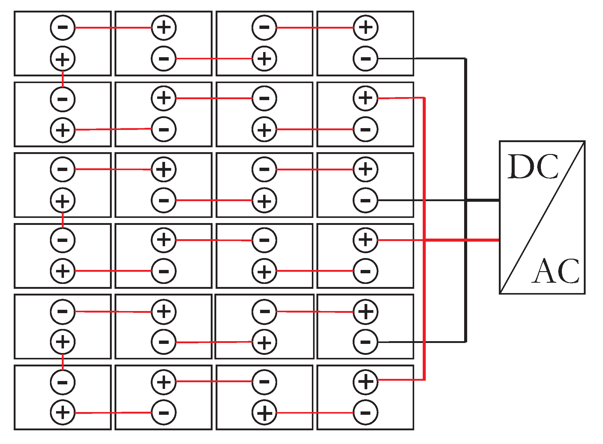
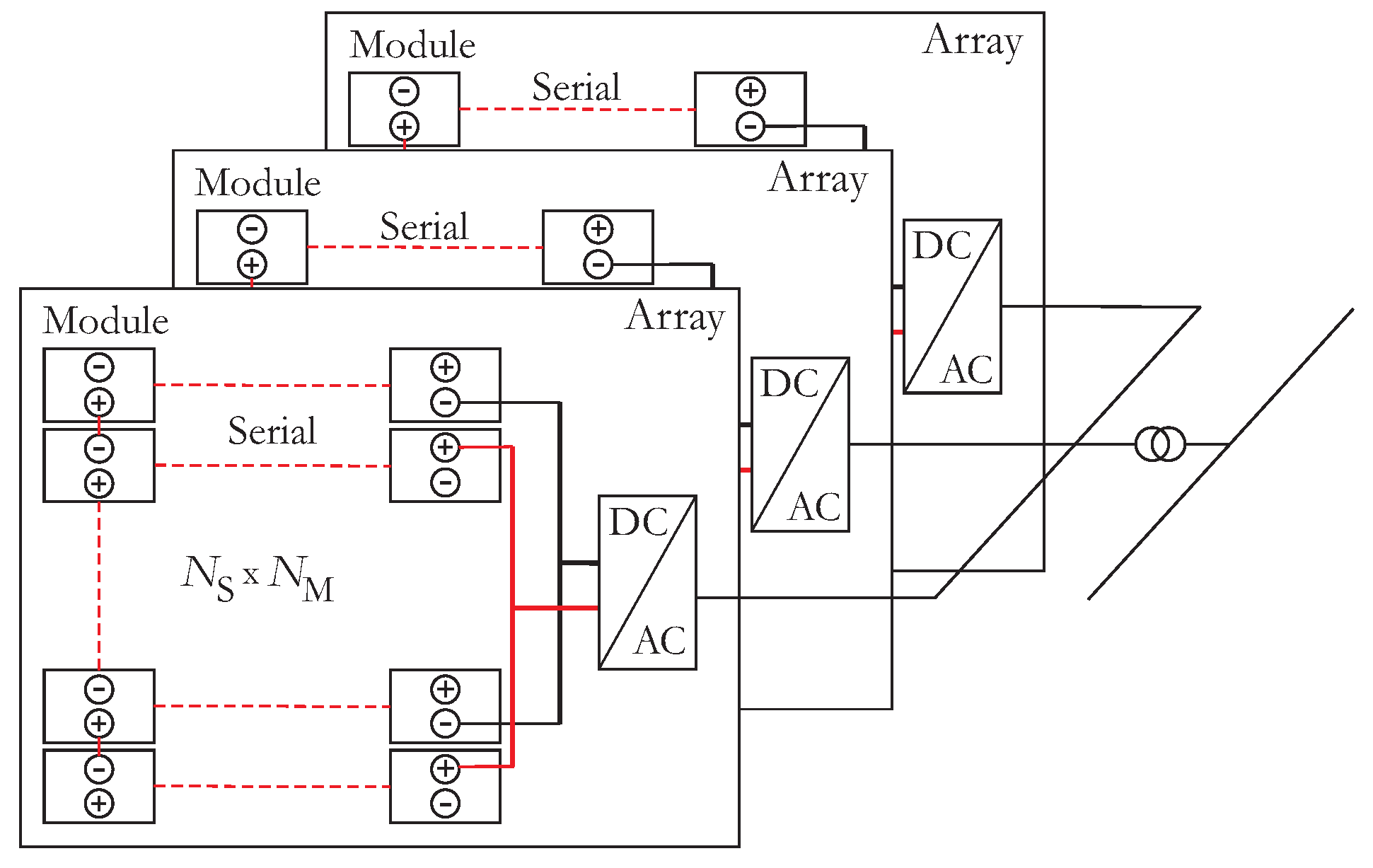
2. Serial-Parallel Topology (SP)

Serial-parallel topology (SP) is realized by connecting the N M modules in series (in so-called “strings”) and then connecting N S strings in parallel, where N S is the number of strings, and N M is the number of modules in the string. The module and the inverter parameters are used to select the number of modules in the strings and the number of strings in parallel. The types of modules and inverter parameters are chosen according to the predicted power of the power plant, that is, the available area [21]. The parameters of the inverter and the solar module for the configuration of SP topology are provided by the manufacturer, as shown in Table 1.
One array is formed as N S × N M , where N S is the number of strings, and N M is the number of modules in the string (Figure 1).
The number of modules in a string can be determined by the equation:
N M = U DC min + U DC max 2 · U PN .
The following condition must be met:
N M · U O < U max .
The number of strings in the array can be calculated as:
N S = P INV N M · G 1000 · P p ,
where G is the maximum insolation at the location of the FPV power plant [W/m2]. P p is the nominal power of the module measured under standard test conditions (insolation 1000 W/m2 and solar cell temperature T C = 25   C ). The number of modules per array is as follows:
N P = N S · N M .
The usable power of the inverter can be calculated:
P INVK = N P · G 1000 P p .
The total number of arrays in the system can be determined by the equation:
N A = P P INVK ,
where P is the predicted power of the plant.
The block structure of one large-scale FPV power plant is presented in Figure 2.
The basic building block is an array that is multiplied N A times, where N A is the number of arrays in the PV plant [21]. The value of N A may vary from a few tens to a few thousand. It can be shown that the system performance is at its maximum when the array performance is at its maximum. This stems from the fact that the system, up to the point of connection to the network, is realized as a simple sum of an array.

3. Array Cabling on the DC Side

Each array is wired on the DC side, where the modules are connected in one of the topologies. The array is connected to the transformer input to the network on the AC side. It is necessary to determine the cable length, cable type, and losses in the cables for one array on the DC side. Depending on the number of inverters and the number of solar modules per inverter, the complexity or values of the listed parameters may differ. The optimal choice of inverter type and solar module type can be challenging [21,22,23]; in this paper, it is assumed that it is defined.

3.1. DC Cabling

The type of DC cable is selected according to the short-circuit current ( I SC ), the maximum system voltage ( U max p ), the ambient conditions ( T a ), and according to the relevant standards [11]. The SP topology requires two types of cable: one that connects the solar modules in a string (S 1 ) and another that connects the strings to the inverter input (S 2 ).
According to the standards, the cable cross-section has to be chosen so that value of its nominal current is 1.56 times the value of the short-circuit current of the solar module [11]. A temperature correction factor is also introduced. For an ambient temperature of 30 C and a maximum temperature of 40 C , a cable of 90 C is chosen, and this factor is 0.58 [10]. The required current capacity of the I C 1 cable (for serial connections) can be determined as follows:
I C 1 = 1.56 · I SC 0.58 .
The required current capacity of the I C 2 cable (for parallel connections) can be determined as follows:
I C 2 = N S · I C 1 .
In order to determine the lengths of DC cables, it is necessary to know the system’s geometry, which is a function of the way the modules are placed. In this paper, only floating photovoltaic plants (FPV) are considered. FPVs are built on water surfaces such as water reservoirs, hydropower plant reservoirs, natural and artificial lakes, sea surfaces, and water channels [24]. Due to the stability of the pad that supports the solar modules, FPVs are usually realized with one solar module on the carrier. The solar module is mounted on a shorter side of the solar module and placed along the carrier’s edge. In addition, the carriers are at the level of the base on which the cables are placed (Figure 3). Due to the vibration of the structure, the modules in the same string are spaced apart for L 0 .
The distance between two arrays is determined by:
D = W ( cos α + sin α · cot β ) = W ( cos α + sin α · tan ( α at + 23.5 ) ,
where α at is the latitude of the location. The cables lengths that connect the solar modules in strings and the solar modules between two strings are determined as follows:
d M M = K T · ( L + L 0 ) ,
d S S = K T · ( D + W sin α ) .
The minimum required lengths are multiplied by the coefficient K T . This is due to the flexibility during installation and the shrinkage of the cables at low temperatures. In this paper, 5 % of the length is added, i.e., K T = 1.05 .
In the standard SP configuration, connecting the solar modules in a string where all the solar modules are arranged in one string requires a return cable that doubles the length of the cable per string. If the number of solar modules in the string is even, then the string is divided into two subsets, and the return cable is not required (Figure 4).

3.1.1. Configuration with Two Types of Cables

In this configuration, all solar modules are connected in one string with one type of cable (S 1 ), and strings are connected in parallel with a different kind of cable (S 2 ).
The length of the cable S 1 in one string is determined as follows:
d S 1 = ( N M 2 ) · d M M + d S S + K T · ( L + d P P ) ,
where d P P is the distance between two arrays intended for cable laying. The length of the type one cable (S 1 ) in one array is determined as follows:
d S = N S · d S 1 + D , N S = 1 4 · D , N S = 2 8 · D , N S = 3 .
For N S = 1 , 2 , and 3 there is no need for a second type of cable in the system. For N S > 3 , a type one cable covers a length of 8 D (one string on each side with width 2 D times 2 for both polarities).
The length of the second cable type in one array is determined as follows:
d S 2 = 4 · D · ( N S 3 ) , N S > 3 0 , N S = 1 , 2 , 3 .
The length of the (+) pole of the cable along the cable tray is 2 D N S D . From this length must be subtracted one width of the string on both sides ( 2 · 2 D ). The factor 2 is used to include the (−) pole of the cable. For a number of strings smaller than 4 ( 1 , 2 , and 3), only one type of cable (S 1 ) is used.
Power is calculated as follows:
P C = R C I 2 ,
where R C is the conductor resistance. The conductor resistance for one string (serial and parallel connection) is as follows:
R C 1 = d S 1 · R 1 ,
R C 2 = d S 2 · R 2 ,
where R 1 and R 2 are the resistances of type 1 and type 2 conductors, respectively. The power losses in the conductors of one string are:
P 1 = R C 1 · I 1 2 ,
where I 1 is the string current. The power losses on the array are:
P 1 u = N S · P 1 .
To determine the power losses in a parallel connection, the scheme in Figure 5 will be used.
R is the resistance of the type 2 conductor between the two strings (S 2 ). Since the distances between the strings is equal and since type two cable is used along the whole cable tray (for parallel connection of arrays), then the resistance is calculated as:
R = R C 2 N S 2 .
The inverter is placed in the middle of the cable tray (later, it is shown that this is the optimal position for power loss on DC cables). It is sufficient to calculate losses on one half of the array. Due to the symmetry of the problem, the total losses will be twice those calculated on half the array.
According to the scheme from Figure 5, the following applies:
P 1 / 2 = R I 1 2 + 2 2 I 1 2 + 3 2 I 1 2 + + N S 2 1 2 I 1 2 = R I 1 2 n = 1 N S 2 1 n 2 = R I 1 2 N S ( N S 1 ) ( N S 2 ) 24 .
Here, the losses are calculated on half of the array. Therefore the result must be multiplied by two, and then by two again, to include the (+) and (−) polarities. Further, R from Equation (20) is replaced, and the expression 8 D · R 1 is added (because the last strings are connected with the first type of cable). Finally, losses on parallel connections are as follows:
P 2 = N S ( N S 1 ) 6 · R C 2 + 8 D · R 1 · I 1 2 , N S > 3 .
In order to connect all strings in parallel, voltage equalization on all strings is required. If a string does not generate enough voltage for any reason, then the currents of the other strings will partly flow over the string with the lowest voltage until the voltages are equalized. This causes losses and the unfavorable operation of the solar modules. Therefore, all strings on the (+) pole are connected by a blocking diode. A Schottky diode is selected as a blocking diode. Diodes are selected according to the string current and string voltage. The voltage drop across this diode for a current of 10 A is 0.55 V [25,26]. The number of diodes in one array is the same as the number of strings. The losses in these diodes are:
P D = N S I 1 U D .
The cables are connected by appropriate connectors whose resistances, according to catalog data, range from 0.1   m Ω to 2 m Ω [27,28,29]. Losses in the connectors are also significant and should be considered. The total number of connectors in one array (with N M solar modules in a string and with N S strings) is:
N K = N S ( N M + 2 ) .
The number of connectors used is as follows: one connector per solar module–solar module connection ( N M 1 ) in the string, one connector for the (−) pole in the parallel connection, one connector for the (+) pole of the anode of the blocking diode, and one connector for the cathode of the blocking diode to the parallel connection. Power losses at the connectors are determined by:
P K = N K · R K · I 1 2 ,
where R K is the resistance of the connectors, and I 1 is the current at the connector that corresponds to the current of the strings.

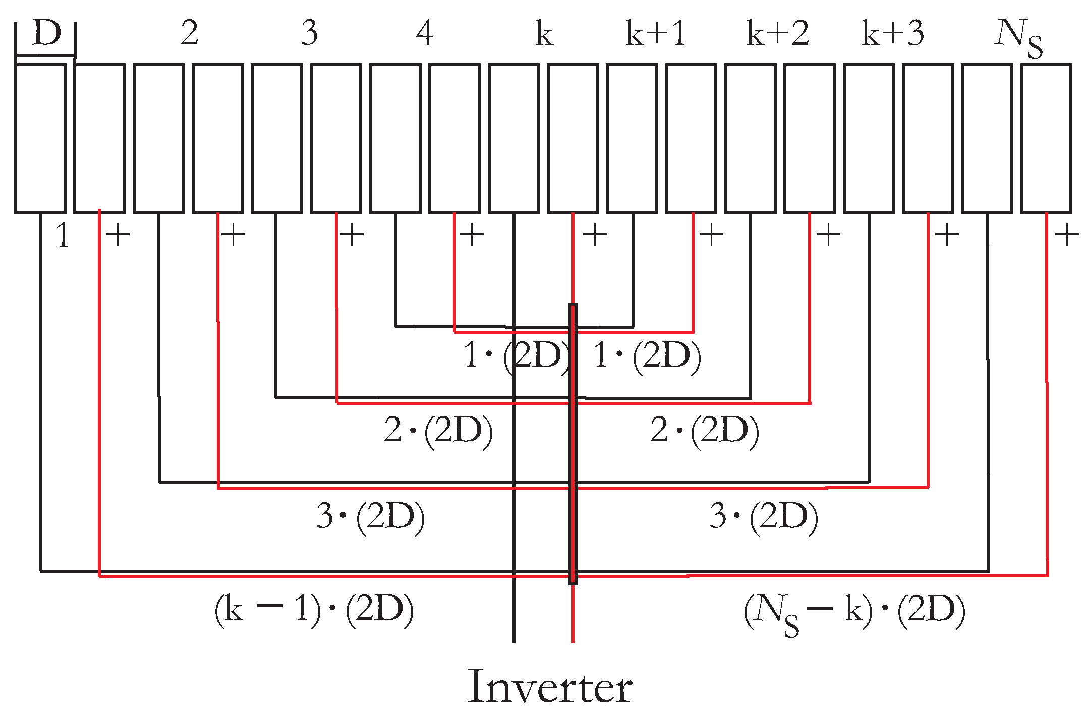
3.1.2. Configuration with One Type of Cable

With one type of cable, strings are connected in the same way as with two cable types. The second type of cable is replaced by connecting the strings to the input of the block for a parallel connection of strings, SCB (String Combiner Box). This block also contains elements of overcurrent protection (fuses), blocking diodes, measuring and monitoring systems, etc. [30]. If the inverter is placed in an array (minimum length of DC cables), then the SCB is placed directly next to the inverter. The cable that connects the SCB and the inverter is then short (with required cross-section), and its losses can be neglected. The conductors of individual strings are connected through one blocking diode ((+) pole) and three connectors (the connection between the cable and the anode of the blocking diode, the connection between the cathode of the blocking diode, and the common point for (+) input to the inverter, the connection between the (−) pole of the string and the common point (−) input in the inverters) to the bus of the inverter input. Therefore, losses on connectors and blocking diodes can be calculated in the same way as with two types of cables. The total length of cables that replace the type 2 cable depends on the position of the inverter. It is shown herein that the minimum length of this part of the cabling is achieved when the inverter is placed in the middle of the cable tray, which connects the strings of one array.
Let it be assumed that the number of strings is N S ( S tr 1 , S tr 2 , S tr 3 , , S tr N S 1 , S tr N S ) , and that the inverter is placed in the middle of the k-th string (Figure 6).
Then, the sum of the lengths of the strings’ distances from the inverter is given by:
d v = 2 D i = 1 k 1 i + 2 D i = 1 N S k i + 2 D i = 1 k 1 i + D k + 2 D i = 1 N S k i D ( N S k ) = 2 · 2 D k ( k 1 ) 2 + 2 · 2 D ( N S k ) ( N S k + 1 ) 2 + 2 D k + D N S = D 4 k 2 4 k N S 2 k + 2 N S 2 + N S .
The first two terms are the sum of the lengths for the (+) pole of the cables, the third and fourth terms are the sum of the lengths for the (−) pole on the left side of the inverter, and the fifth and sixth terms are the sum of the lengths for the (−) pole on the right side of the inverter. The result is a quadratic function of k. The minimum is obtained for 4 k 2 N S 1 = 0 , and then k can be expressed as follows:
k = N S 2 + 1 4 .
It is shown that the optimal location of the inverter is in the middle of the cable tray when a minimum cable length on the DC side is required. In Equation (27), 1 / 4 is a consequence of string widths and asymmetry of (+) and (−) cable lengths.
Let it be assumed that k = N S / 2 , that is, the inverter is in the middle of the cable tray. By replacing k in Equation (26), the total length of the cable in the cable tray is:
d v = N S 2 · D , N S > 3 .
The cable length in one array is:
d P = d S + d v ,
where d S is determined by Equation (13).

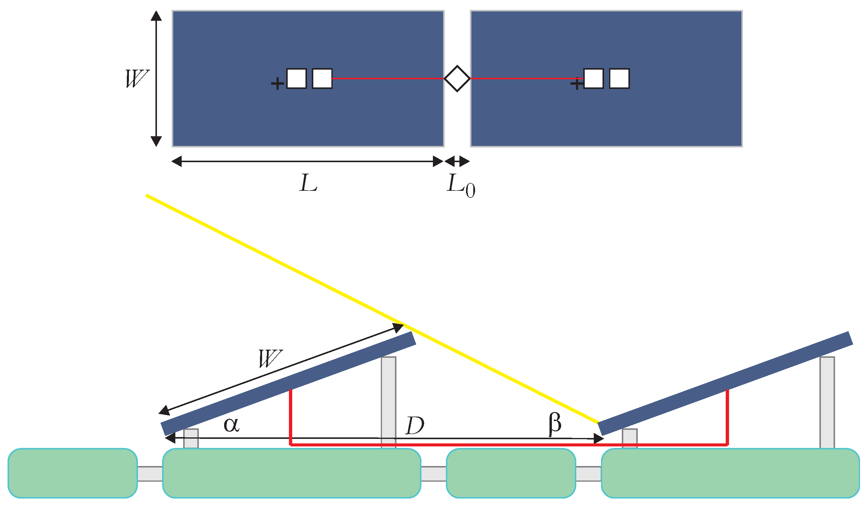
3.1.3. Array Geometry

Each array is represented as a rectangle of sides a and b. In addition, it is assumed that the number of solar modules per string is even. Then, sides a and b are determined as:
a = ( L + L 0 ) · N M 2 + d P P 2 ,
b = 2 D · N S .

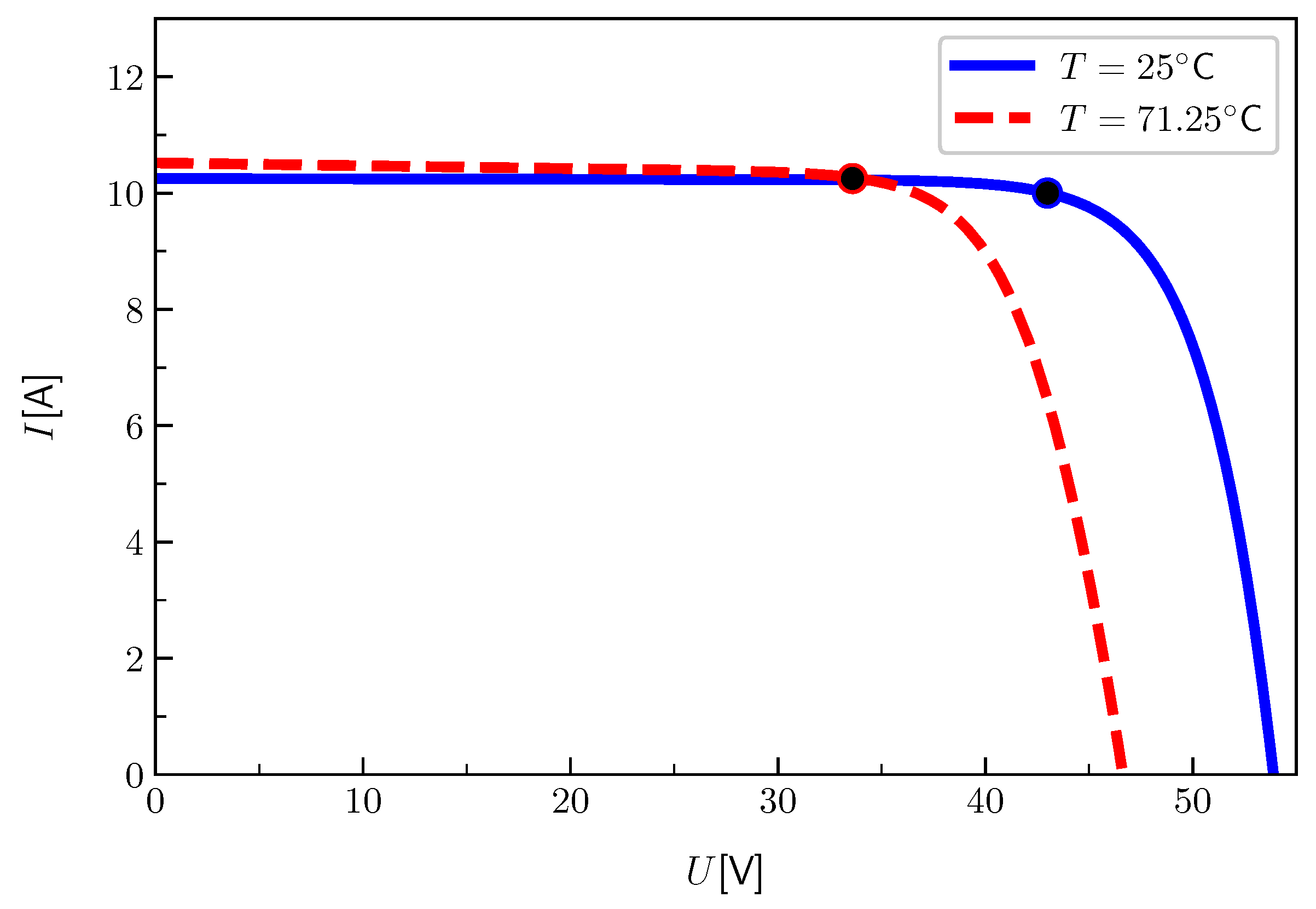
4. Impact of Temperature on Cable Losses

Temperature is an important parameter when considering the operation of PV systems [31,32,33,34,35]. The temperature changes the parameters of the solar module ( I SC , U O , P P ) as well as the resistances of the DC conductors R 1 and R 2 . Solar modules are tested for current, voltage, and power under standard conditions (STC) of 1000 W/m2 insolation and 25 C solar cell temperature. For these values, catalog data are given for modules; such data includes short-circuit current I SC , open-circuit voltage U O , maximum power P P , operating current at maximum power I PN , and operating voltage at maximum power U PN . The power plant operates in a temperature range that can vary from 20   C to 45 C . The relations that connect the catalog data with the real data are given below [33,34,35]:
I SC ( T , G ) = I SC , STD · 1 + k i 100 ( T C 25 C ) · G 1000 ,
U O ( T ) = U O , STD · 1 + k u 100 ( T C 25 C ) ,
P ( T ) = P P , STD · 1 + k p 100 ( T C 25 C ) ,
F F = I PN · U PN I SC · U O .
A nominal operating temperature of a solar cell is measured for insulation 800 W/m2 and 20 C ambient temperature. For these values, the nominal temperature of the cell (NCOT) is given as catalog data.
T C = T a + NCOT 20   C 800   W / m 2 · G .
Cell temperature T C can be calculated by Equation (36) if the insolation G, the ambient temperature T a , and the NCOT are known. The short-circuit current and open-circuit voltage at this cell temperature can be determined according to Equations (32) and (33). There is a change in the current-voltage characteristic of the solar panel and thus a change in the operating point compared to the nominal point. The current and voltage ( I 1 , U 1 ) at the point of maximum power at this temperature are different compared to the nominal values ( I PN , U PN ). This change is a linear function of temperature [34] and depends on the temperature coefficients. Temperature coefficients can be represented as a linear combination of the catalog coefficients k i and k u , so Equations (32) and (33) can be written:
I 1 ( T , G ) = I PN · 1 + γ k i 100 ( T C 25 C ) · G 1000 ,
U 1 ( T ) = U PN · 1 + θ k u 100 ( T C 25 C ) .
Power as a function of cell temperature is determined by Equation (34) if the catalog parameter k p , nominal power P p , and cell temperature T C are known [34]. The same value of power is given by the product of current and voltage at that temperature obtained by Equations (37) and (38) [36].
This gives the relation of the coefficients k i ,   k u ,   k p ,   γ k i ,   θ k u as follows:
k p = γ · k i + θ · k u + γ · k i · θ · k u T C 25 C 100 .
The coefficients γ k i and θ k u are coefficients of change in current and voltage at the maximum power point (MPP) as a function of temperature. Equation (39) express the fact that coefficients γ k i and θ k u depend on temperature if k p is treated as a constant coefficient. Without the established ratio of the factors γ and θ , Equation (39) cannot be applied to determine the change in current as a function of temperature at the maximum power point. In determining this relationship, it is necessary to start with the definition of temperature coefficients. The temperature coefficients of power, current, and voltage are the quotients of power change and temperature change, current change and temperature change, and voltage change and temperature change, respectively:
k p = 100 P T d P d T , γ k i = 100 I T d I d T , θ k u = 100 U T d U d T ,
where the measuring unit of coefficients k p , k u , and k i is [ %/ C ], and P T , U T , and I T are values of power, voltage, and current, respectively, in the specific point. For the maximum power point, using Equation (40), the following applies [36]:
k p = 100 P T d d T ( U · I ) = 100 P T d U d T I + 100 P T d I d T U = θ k u I I T + γ k i U U T .
The coefficients from Equation (40) refer to any point of the UI characteristic curve and represent the percentage change in power, current, and voltage as a function of temperature in relation to the value of power, current, and voltage at that point. By normalizing these coefficients to the unit amount of power, current, and voltage, we obtain these coefficients for any point. This means that in Equation (41) we set P T = 1   W , U T = 1   V , and I T = 1   A . Now Equation (41) becomes
k p = θ k u I [ A 1 ] + γ k i U [ V 1 ] .
Equalizing Equations (39) and (42), and neglecting expressions with small values (product of k u and k i ) the ratio of γ and θ is obtained as follows:
γ k i θ k u = 1 U PN · 1 / V I PN · 1 / A 1 .
U and I are replaced by U PN and I PN because the change in current as a function of temperature change at the maximum power point according to STC conditions is calculated. By including Equation (43) in Equation (39), γ is determined as follows:
γ = ( 1 + B ) ( 1 + B ) 2 + 4 · k p · B · T C 25 C 100 2 · B · k i · T C 25 C 100 , B = 1 U PN · 1 / V I PN · 1 / A 1 .
The problem with the temperature coefficients of current and voltage was discussed in [37]; catalog data is provided only for short-circuit current and open-circuit voltages but not for other points on the current-voltage characteristic. It was found that some authors use the same coefficient for the whole characteristic, but that is not justified [38]. It is proposed to determine this coefficient by measuring in specific conditions. It is also evident that temperature coefficients change with insolation [36,38].
For the following values of coefficients k i = 0.05 % C 1 , k u = 0.29 % C 1 , k p = 0.37 % C 1 , and ambient temperature of 35 C , γ = 1.707862 is calculated. Figure 7 presents the change in characteristic values ( I SC , U O , I 1 , U 1 ) for cell temperatures between 25 C and 71.25   C at 1000 W/m2 of insolation. For a temperature of 25 C , the obtained values are as follows: I SC = 10.25   A , U 0 = 53.9   V , P P = 440   W , U 1 = 44.56   V , and I 1 = 9.65   A . These values correspond to the catalog data under STC conditions. For a temperature of 71.25   C , the values are I SC = 10.49   A , U 0 = 46.67   V , P P = 364.71   W , U 1 = 39.45   V , and I 1 = 9.87   A .
I SC and U O are catalog values, while I 1 and U 1 are obtained according to Equations (37) and (38), where γ is determined by Equation (44).
Table 2 shows the changes in solar module voltage at the maximum power point, the solar module current at the maximum power point, the cell temperature, and the coefficient γ as a function of ambient temperature changed from 10   C to 50 C . It is assumed that the insolation is 1000 W/m2.
The results of different methods of determining the values of current, voltage, and power as a function of temperature at the maximum power point and for G = 1000   W / m 2 are given in Table 3.
Columns 2 and 3 represent the calculated values of currents and voltages with correction of the coefficients k i and k u by the factors γ and θ . Columns 4 and 5 represent the calculated values of currents and voltages without correction of the coefficients k i and k u , ( γ = 1 and θ = 1 ). Column 6 represents the power calculated based on currents and voltages determined without coefficients γ and θ (columns 4 and 5). Column 7 represents the power calculated based on the nominal power and the coefficient k p . Column 8 represents the power calculated based on the current and voltage with coefficients γ and θ (columns 2 and 3). Column 7 corresponds to the closest power values because it is determined based on catalog data specified by the manufacturer. Power data calculated according to the proposed method are given in column 8, and the absolute error is below 0.09 % . Column 6 represents the data according to the catalog coefficients k i and k u given for the short-circuit current I SC and the open-circuit voltage U O . The maximum absolute error for column 6 is 8.58 % . Based on previous results, the correction of the coefficients k i and k u should be performed when calculating currents and voltages outside the points ( 0 , I SC ) and ( U O , 0 ) .
The change in resistance according to the change in temperature is determined by:
R = R 0 ( 1 + α T · ( T T 0 ) ) ,
where R 0 is the resistance at room temperature T 0 ( 25 C ), T is the operating resistance temperature, and α T is the temperature coefficient. The temperature coefficient of copper is 0.00392 °C−1. If the ambient temperature ( T a ) is known, it can be assumed that the temperature of the cable at operating current ( I 1 ) will be equal to or lower than the cell temperature. The cell’s temperature is determined based on the energy of solar radiation, which is converted into thermal energy on the cell, plus thermal energy, which is released on the cable inside the solar module due to the flow of the current. The conductors between the modules are connected to the cables on the solar module. This leads to heat transfer from the solar module (which is warmer) to the cables. In addition to this heat, the cables are also heated due to the current flowing through them. The value of the resistance of the cable at ambient temperature can be determined according to:
R = R 0 ( 1 + α T · ( T C T 0 ) ) .
Considering these corrections to the resistance amounts R 1 and R 2 , the estimation of losses can be obtained with the ambient temperature taken into consideration as follows:
R 1 ( T a ) = R 1 ( 1 + 0.00392 · ( T C T 0 ) ) ,
R 2 ( T a ) = R 2 ( 1 + 0.00392 · ( T C T 0 ) ) .
The cables have standard cross-sections and resistances whose values are given by the manufacturers (Ω km−1). In addition to the stated values, data on nominal cable currents and linear mass density for copper and aluminum are given in Table 4 [27].
For economic reasons, using aluminum instead of copper may be an option. Table 4 shows, in addition to the parameters of copper conductors, the parameters of aluminum conductors for larger amounts of current I N . When replacing a copper conductor with an aluminum one, the same current capacity should be provided. This requires equivalents with a larger cross-section, as indicated in the table, so an aluminum conductor with a cross-section of 95 m m 2 is used in place of a 35 m m 2 copper conductor cross-section, with comparable nominal currents of 218 A and 216 A . The longitudinal resistance of aluminum conductors with this cross section is less than the resistance of the equivalent copper conductors. The same applies to the other substitute values listed in Table 4.

5. Testing of the Model/Case Study

To test the DC cabling model, a hypothetical power plant with a nominal power of 3 MW is considered. The PV plant is conceived as N A arrays, where each array contains N S × N M solar panels connected in a serial-parallel configuration. The total array power is matched to the power of the selected inverter by choosing the N S × N M configuration so that N S × N M × P P P INV , where P P is the nominal power of the selected panel and P INV is the nominal power of the selected inverter. All inverters are connected on the AC side to the input bus of the transformer, which connects the plant to the power system. The input data depend on the type of solar modules, and the model is made to support changes in all input data. The inputs to the model are the parameters given in Table 5.
The output results are presented in Table 6, where the solar module HCM78 × 9–440 W [40] and a 16 kw power inverter are used.
The output data can be used for techno-economic analysis, feasibility studies, design, etc. The power losses on the DC cables were specifically analyzed. Figure 8 shows the results of the simulation of losses on the DC cables as a function of the nominal power of the inverter.
The ambient temperature is 35 C , and insolation is 1000 W/m2. The power of the inverter is changed from 5300 W to 90,100 W in increments of 5300 W . Under these conditions, the power efficiency of the inverter exceeds 99 % . The blue curve denoted by p 1 represents the results for cabling with two types of cables. For this cabling method, power losses on the DC cables do not exceed 0.55 % . The red-dashed curve ( p 2 ) represents the cabling results with only one type of cable. With increasing power, the losses increase linearly and are larger than those with two types of cables. The maximum value is obtained for an inverter power of 90,100 W and is equal to 0.71 % .
Table 7 shows the economic parameters of DC cabling for inverters with different power levels.
For a topology with two cable types, the S 1 cable is 4 mm2, with an average cable length of 18.3 km and an average cable copper mass (M) of 702 k g . The average value of the cable length and the cable copper mass is calculated for the different power inverters, using the values from columns 2 and 3 of Table 7. The S 2 cable has cross-sections ranging from 16 mm2 to 120 mm2, lengths ranging from 1 km to 3.3 km, and copper masses ranging from 156 k g to 3815 k g . The one-cable topology uses an S 1 cable with a 4 mm2 cross-section, an average length of 20.4 km, and an average cable copper mass of 785 k g , where average length and mass values are calculated using columns 7 and 8 of Table 7. Based on the above data, it is possible to calculate the cost-effectiveness of investing in copper to reduce losses. It is necessary to decide between a topology with one type of cable and a topology with two types of cables.

6. Conclusions

This paper presents a general method for calculating the length and type of cables on the DC side of large-scale floating photovoltaic power plants. Power losses in cables are analyzed. It is demonstrated that losses are less than 0.55 % for the topology with two types of cables and increase slightly with an increase in the power of the inverter. With a one-cable type topology, power losses are higher, up to 0.7 % , and they increase faster with an increase in the power of the inverter. If the number of strings is greater than three, a topology with two types of cables should be used. If the number of strings is three or fewer, it is sufficient to use only one cable type.
This paper develops a method for the calculation of cable lengths and power losses in cables, as well as a method for analyzing the techno-economic parameters of power plants, such as the number of modules, the number of inverters, the number of connectors, the number of blocking diodes, the required area, the cable types, the copper mass on DC cables, etc.
For power loss calculation, this model considers the change in current and resistance as a function of temperature. The coefficient of change in the short-circuit current as a function of the temperature is given in the catalog. Still, the catalog does not provide data about the current change at the maximum power point.
This paper shows how the current change can be determined at the maximum power point depending on the temperature. We obtain an expression for current and voltage calculation at the operating point as a function of temperature. To use that expression, a correction factor that multiplies the temperature coefficient of the current must be used. This factor slightly depends on the temperature change, and its average value is 1.734992 . By applying this coefficient, the power calculation at the maximum power point differs from the value obtained using catalog data for k p by less than 0.09 % .
In this paper, only losses on DC conductors are analyzed. However, in the DC array, there are other losses that occur as a result of the system operating in real conditions. Parallel and series connections of solar modules in configurations adapted to the parameters of the used inverters lead to the equalization of currents of solar modules connected in a string and the equalization of voltages at the ends of strings connected in parallel operation. Any asymmetry, i.e., a deviation of the operating conditions of an individual solar module from the others in the group, reduces the performance of the system due to these equalizations. This reduction is manifested by the working point of the solar panels being moved beyond the point of the MPP due to alignment with the other panels in the array. This problem is especially pronounced when individual strings in parallel, or modules in a string, do not have the same insolation, i.e., when a shadow appears on a part of the plant. Significant losses then occur, and this problem is the subject of intensive research, where different wiring topologies are analyzed in terms of their potential to reduce these losses. In this paper, we have not dealt with this problem; instead, we assume identical conditions for all panels in the system. In addition, different string positions relative to the inverter require different cable lengths. This leads to different voltage drops on the cables, and losses occur due to voltage equalization in parallel connections. These losses are not large because differences in line lengths occur only on parallel connections that have larger cross-sections and shorter lengths. The problem is that these losses occur constantly and not occasionally, as in shading. In any case, the problems of losses due to voltage drops and shading are important and should be analyzed in future research.

Author Contributions

Conceptualization, A.A. and S.K.; methodology, A.A., S.P. and S.O.; investigation, A.A., S.P. and S.G.; data curation, S.K.; software, S.O.; visualization, S.O. and S.G.; writing—original draft preparation, A.A., S.K. and S.O.; writing—review and editing, S.O. All authors have read and agreed to the published version of the manuscript.

Funding

This research was funded by the Federal Ministry of Education and Science, Bosnia and Herzegovina, grant No. 05-35-1966-1/21.

Institutional Review Board Statement

Not applicable.

Informed Consent Statement

Not applicable.

Data Availability Statement

The data underlying this study are available on reasonable request to the corresponding author.

Acknowledgments

We wish to express our gratitude to the Faculty of Science and the Faculty of Electrical Engineering of the University of Sarajevo for providing equipment and assistance in the implementation of the research.

Conflicts of Interest

The authors declare no conflict of interest.

References

  1. Pašalić, S.; Akšamović, A.; Avdaković, S. Floating photovoltaic plants on artificial accumulations—Example of Jablanica Lake. In Proceedings of the 2018 IEEE International Energy Conference (ENERGYCON), Limassol, Cyprus, 3–7 June 2018; pp. 1–6. [Google Scholar] [CrossRef]
  2. Nuñez-Jimenez, A.; Bkayrat, R. Utility scale 1500 VDC PV power plant architecture evolution: Advantages and challenges. In Proceedings of the Integration of Renewable Energy into High and Medium Voltage Systems Conference & Exhibition, Amman, Jordan, 15–16 September 2015. [Google Scholar]
  3. Cabrera-Tobar, A.; Bullich-Massagué, E.; Aragüés-Peñalba, M.; Gomis-Bellmunt, O. Topologies for large scale photovoltaic power plants. Renew. Sustain. Energy Rev. 2016, 59, 309–319. [Google Scholar] [CrossRef] [Green Version]
  4. Blueplanet 87.0—150 TL3 Transformerless, Three-Phase String Inverters. Available online: https://bit.ly/KacoNewEnergy (accessed on 20 December 2021).
  5. Decentralized Inverter Technology in Large-Scale PV Plants. Available online: https://bit.ly/SMAinverter (accessed on 20 December 2021).
  6. Shah, R.; Mithulananthan, N.; Bansal, R.; Ramachandaramurthy, V. A review of key power system stability challenges for large-scale PV integration. Renew. Sustain. Energy Rev. 2015, 41, 1423–1436. [Google Scholar] [CrossRef]
  7. Stoyanov, I.S.; Iliev, T.B.; Mihaylov, G.Y.; Evstatiev, B.I. Modelling of power inverters used in PV systems. In Proceedings of the 2017 IEEE 23rd International Symposium for Design and Technology in Electronic Packaging (SIITME), Constanta, Romania, 26–29 October 2017; IEEE: Piscataway, NJ, USA, 2017. [Google Scholar] [CrossRef]
  8. IEC MSB. Grid Integration of Large-Capacity Renewable Energy Sources and Use of Large-Capacity Electrical Energy Storage; IEC MSB: Geneva, Switzerland, 2012; pp. 1–102. [Google Scholar]
  9. Pachauri, R.K.; Mahela, O.P.; Sharma, A.; Bai, J.; Chauhan, Y.K.; Khan, B.; Alhelou, H.H. Impact of Partial Shading on Various PV Array Configurations and Different Modeling Approaches: A Comprehensive Review. IEEE Access 2020, 8, 181375–181403. [Google Scholar] [CrossRef]
  10. Khan, F.U.; Murtaza, A.F.; Sher, H.A.; Al-Haddad, K.; Mustafa, F. Cabling Constraints in PV Array Architecture: Design, Mathematical Model and Cost Analysis. IEEE Access 2020, 8, 182742–182754. [Google Scholar] [CrossRef]
  11. Wiles, J. Photovoltaic Power Systems and the National Electrical Code: Suggested Practices; Sandia National Labs.: Livermore, CA, USA, 2001. [Google Scholar] [CrossRef] [Green Version]
  12. Technical Application Papers No. 10 Photovoltaic Plants. Available online: https://bit.ly/ABBTechnicalApplication (accessed on 20 December 2021).
  13. Malamaki, K.N.D.; Demoulias, C.S. Minimization of Electrical Losses in Two-Axis Tracking PV Systems. IEEE Trans. Power Deliv. 2013, 28, 2445–2455. [Google Scholar] [CrossRef]
  14. Malamaki, K.N.D.; Demoulias, C.S. Analytical Calculation of the Electrical Energy Losses on Fixed-Mounted PV Plants. IEEE Trans. Sustain. Energy 2014, 5, 1080–1089. [Google Scholar] [CrossRef]
  15. Ziar, H.; Farhangi, S.; Asaei, B. Modification to Wiring and Protection Standards of Photovoltaic Systems. IEEE J. Photovoltaics 2014, 4, 1603–1609. [Google Scholar] [CrossRef]
  16. Gan, C.K.; Lee, Y.M.; Pudjianto, D.; Strbac, G. Role of losses in design of DC cable for solar PV applications. In Proceedings of the 2014 Australasian Universities Power Engineering Conference (AUPEC), Perth, WA, Australia, 28 September–1 October 2014; pp. 1–5. [Google Scholar] [CrossRef]
  17. Şenol, M.; Abbasoğlu, S.; Kükrer, O.; Babatunde, A. A guide in installing large-scale PV power plant for self consumption mechanism. Sol. Energy 2016, 132, 518–537. [Google Scholar] [CrossRef]
  18. El-Hafez, O.J.; ElMekkawy, T.Y.; Kharbeche, M.B.M.; Massoud, A.M. Economic Energy Allocation of Conventional and Large-Scale PV Power Plants. Appl. Sci. 2022, 12, 1362. [Google Scholar] [CrossRef]
  19. Stoyanov, I.; Ivanov, V.; Iliev, T.; Ivanov, H. Yield and Performance Study of a 1MWp Grid Connected Photovoltaic System in Bulgaria. J. Eng. Sci. Technol. Rev. 2019, 206–209. [Google Scholar]
  20. Bullich-Massagué, E.; Cifuentes-García, F.J.; Glenny-Crende, I.; Cheah-Mañé, M.; Aragüés-Peñalba, M.; Díaz-González, F.; Gomis-Bellmunt, O. A review of energy storage technologies for large scale photovoltaic power plants. Appl. Energy 2020, 274, 115213. [Google Scholar] [CrossRef]
  21. Kornelakis, A.; Koutroulis, E. Methodology for the design optimisation and the economic analysis of grid-connected photovoltaic systems. Renew. Power Gener. IET 2010, 3, 476–492. [Google Scholar] [CrossRef]
  22. Faranda, R.; Hafezi, H.; Leva, S.; Mussetta, M.; Ogliari, E. The optimum PV plant for a given solar DC/AC converter. Energies 2015, 8, 4853–4870. [Google Scholar] [CrossRef]
  23. Alsadi, S.; Khatib, T. Photovoltaic Power Systems Optimization Research Status: A Review of Criteria, Constrains, Models, Techniques, and Software Tools. Appl. Sci. 2018, 8, 1761. [Google Scholar] [CrossRef] [Green Version]
  24. Acharya, M.; Devraj, S. Floating Solar Photovoltaic (FSPV): A Third Pillar to Solar PV Sector; The Energy and Resources Institute: Mithapur, India, 2019; Available online: https://bit.ly/AcharyaEnergy2019 (accessed on 3 May 2020).
  25. EIC Diodes in Solar Photovoltaic (PV) Systems. Available online: https://bit.ly/EICdiodes (accessed on 20 December 2021).
  26. How to Choose a Bypass Diode for a Silicon Panel Junction Box. Available online: https://bit.ly/DiodeSTM (accessed on 20 December 2021).
  27. Cables and Cable Systems for Photovoltaic Installations. Available online: https://bit.ly/Helukabel (accessed on 20 December 2021).
  28. Solar Connectors and Cable Assemblies. Available online: https://bit.ly/AmphenolConnectors (accessed on 20 December 2021).
  29. DC Cabling Ready for 1500 V DC. Available online: https://bit.ly/JurchenTechnology (accessed on 20 December 2021).
  30. Solar String Combiner for PV Application. Available online: https://bit.ly/ABBSolarString (accessed on 20 December 2021).
  31. Singh, P.; Ravindra, N. Temperature dependence of solar cell performance—An analysis. Sol. Energy Mater. Sol. Cells 2012, 101, 36–45. [Google Scholar] [CrossRef]
  32. Radziemska, E.; Klugmann, E. Thermally affected parameters of the current–voltage characteristics of silicon photocell. Energy Convers. Manag. 2002, 43, 1889–1900. [Google Scholar] [CrossRef]
  33. Chander, S.; Purohit, A.; Sharma, A.; Arvind; Nehra, S.; Dhaka, M. A study on photovoltaic parameters of mono-crystalline silicon solar cell with cell temperature. Energy Rep. 2015, 1, 104–109. [Google Scholar] [CrossRef] [Green Version]
  34. Skoplaki, E.; Palyvos, J. On the temperature dependence of photovoltaic module electrical performance: A review of efficiency/power correlations. Sol. Energy 2009, 83, 614–624. [Google Scholar] [CrossRef]
  35. Sera, D.; Teodorescu, R.; Rodriguez, P. PV panel model based on datasheet values. In Proceedings of the 2007 IEEE International Symposium on Industrial Electronics, Vigo, Spain, 4–7 June 2007; pp. 2392–2396. [Google Scholar] [CrossRef]
  36. King, D.; Kratochvil, J.; Boyson, W. Temperature coefficients for PV modules and arrays: Measurement methods, difficulties, and results. In Proceedings of the Conference Record of the Twenty Sixth IEEE Photovoltaic Specialists Conference—1997, Anaheim, CA, USA, 29 September–3 October 1997; pp. 1183–1186. [Google Scholar] [CrossRef] [Green Version]
  37. King, D.; Kratochvil, J.; Boyson, W. Photovoltaic Array Performance Model; Sandia National Laboratories (SNL): Albuquerque, NM, USA; Livermore, CA, USA, 2004. [Google Scholar] [CrossRef] [Green Version]
  38. King, D.L. Photovoltaic module and array performance characterization methods for all system operating conditions. AIP Conf. Proc. 1997, 394, 347–368. [Google Scholar] [CrossRef]
  39. Solar Cables 1.5 kV DC. Available online: https://www.cablegrid.com.au/solar-cables-1-5kv-dc/ (accessed on 21 April 2022).
  40. Half Cell 440w Black Mono Solar Panel. Available online: https://bit.ly/DAHSolar (accessed on 20 December 2021).
Figure 1. Serial–Parallel (SP) topology N S × N M for N S = 3 and N M = 8 .
Applsci 12 04500 g001
Figure 2. Block structure of large-scale FPV power plant.
Applsci 12 04500 g002
Figure 3. Solar module position geometry in FPV plants.
Applsci 12 04500 g003
Figure 4. DC cabling of a string by dividing it into two subsets.
Applsci 12 04500 g004
Figure 5. Scheme of losses on the cables on the DC side.
Applsci 12 04500 g005
Figure 6. Determining the cable length of parallel connections for one type of cable.
Applsci 12 04500 g006
Figure 7. Change in the characteristic values of current and voltage of the solar module for cell temperatures 25 C (solid blue line) and 71.25 C (red dashed line).
Applsci 12 04500 g007
Figure 8. Diagram of power losses on the DC cables as a function of inverter power for both types of cabling.
Applsci 12 04500 g008
Table 1. Inverter and solar module parameters.
Inverter ParametersLabel
Power P INV
Maximum DC input voltage U max
Minimum operating voltage U DC min
Maximum operating voltage U DC max
Maximum input current I IN
Solar Module ParametersLabel
Maximum power P p
Maximum power voltage due to MPP U PN
Maximum power current due to MPP I PN
Open-circuit voltage U O
Short-circuit current I SC
Maximum system voltage U max p
Current temperature coefficient k i
Voltage temperature coefficient k u
Power temperature coefficient k p
Nominal operating cell temperatureNOCT
Dimensions L × W
Table 2. Change in solar panel parameters with change in temperature.
T a [ C] T C [ C] U 1 [V] I 1 [A] γ
10 21.2546.359.621.789966
031.2544.269.701.770358
1041.2542.229.781.751579
2051.2540.229.861.733567
3061.2538.269.951.716263
4071.2536.3410.031.699619
5081.2534.4510.121.683589
Table 3. Three different methods of calculating the power of the solar module at the maximum power point as a function of temperature.
T a [ C] γ = 1.789966 γ = 1 P [W]
I 1 [A] U 1 [V] I 1 [A] U 1 [V]123
−109.6246.349.6346.05443.6446.1445.7
09.7044.269.6844.73433.0429.8429.5
109.7842.229.7343.41422.3413.5413.2
209.8740.229.7842.09411.5397.3397.0
309.9538.269.8240.77400.6381.0380.7
4010.0336.349.8739.45389.5364.7364.4
5010.1134.459.9238.13378.3348.4348.2
Table 4. Parameters of standard cables (data from [27,39]).
CopperAluminum
S
[mm 2 ]
R l
[ Ω /km]
I N
[A]
Linear Density Mass [kg/km] S
[mm 2 ]
R l
[ Ω /km]
I N
[A]
Linear Density Mass [kg/km]
2.57.984124
44.955538.4
63.307057.6
101.919896
161.21132153.6
250.78176240
350.554218336950.32216430
500.3862764801200.253253510
700.2723476721850.164340760
950.2064169122400.125408960
1200.16148811523000.14731160
Table 5. Input data of the model.
HCM78 × 9–440 W Solar
Module Parameters
Inverter Parameters
P P 440 W P INV 16,000 W
U O 53.9   V U DC min 320 V
U PN 45.56   V U DC max 800 V
I SC 10.25   A Efficiency 98.4 %
I PN 9.65   A U NN , max 750 V , AC
k i 0.05 %/ C U max 1000 V
k u 0.29 %/ C
k p 0.37 %/ C
NOCT45 C
Length, L 2.172   m
Width, W 1.002   m
Plant power, P3 MW
Location parameters
Geographic latitude43
Temperature35 C
Insolation, G1000 W/m2
Orientation and distance of the solar modules
Solar module slope angle, α 22
Distance between solar modules, L 0 0.2   m
Distance between modules1   m
Table 6. Output data of the model.
Geometry of ArrayGeometry of System
Array width, b 10.75   m System width 132.6   m
Array length, a 14.73   m System length 225.8   m
Array surface, A 158.42   m 2System surface29,942 m 2
System component data
Number of inverters189Number of arrays189
Number of solar modules6804Number of solar modules in the array36
Number of connectors7938Number of solar modules in the string12
Number of blocking diodes567Number of strings in the array3
CablesLengthCross-sectionMass
Type 120,010.62 m4 m m 2 168.68   k g
Type 20 m
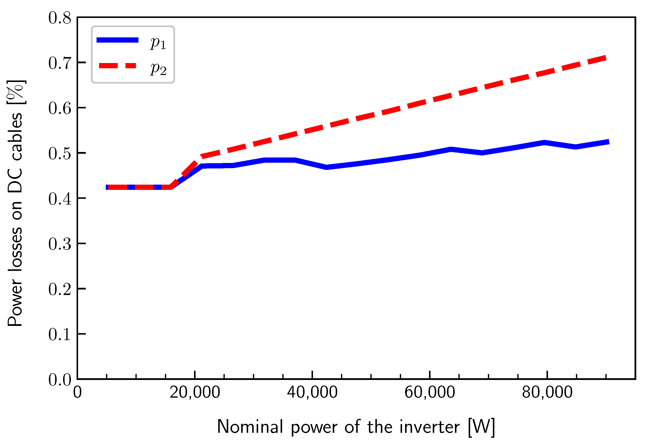
Power losses on DC cabling 0.4239 %
Table 7. Cable lengths, types, and masses for different inverter power levels.
P [kW]Two Types of CablesOne Type of Cable
S 1 , 4 mm 2 S 2 S 1 , 4 mm 2
d [m]M [kg]s [mm 2 ]d [m]M [kg]d [m]M [kg]
5.318,34970418,349704
10.619,36774319,367743
15.920,01076820,010768
21.219,36774316101815620,385782
26.518,85972425162038820,480786
31.818,55671225202148520,578790
37.118,46270835232278020,784798
42.418,349704502545122120,894802
47.718,203699502709130020,913803
5317,890686502810134820,700794
58.317,848685702925196520,773797
63.617,883686703032203720,915803
68.917,673678953082281120,755797
74.217,660678953154287620,815799
79.517,465670953183290320,648792
84.817,5886751203261375720,850800
90.117,5906751203312381520,902802
Publisher’s Note: MDPI stays neutral with regard to jurisdictional claims in published maps and institutional affiliations.

