1. Introduction
1.1. Motivation
Railway networks can ensure environmentally friendly transportation for both passengers and freight traffic. Due to the climatic targets, an increase in the volume transported by rail and average speed is desirable. Accordingly, the main objectives of the European Union are greening the freight transport by doubling rail freight traffic by 2050, boosting the innovation in the sector and bring the data-based solutions and artificial intelligence in the fore [
1]. The possible data-driven solutions in the field of energy efficiency and their future are detailed in [
2]. In addition, reinforcement learning is also an important part of artificial intelligence from an optimization point of view, which can also provide a solution to several challenges in the field of rail transportation, as summarized in [
3]. One such major challenge is how to increase the capacity of the railway lines to achieve these goals. In urban areas, the number of tracks is limited and not expendable at reasonable costs. The first possibility to increase the volume is the density of scheduled trains. However, this method can cause more delays, waiting times, and decreased average speed in disturbing situations. Despite this, real-time automated rescheduling of trains may help increase the railway lines’ capacity. Other capacity-raising methods are the expensive automatic train control (ATC) and automatic train operation (ATO) to minimize driver errors. This method can help operators to make the right decisions to schedule. This process means reordering and rescheduling tasks in a perturbed situation based on railway safety regulations— route-based interlocking rules. Every deviation from the pre-planned conflict-free timetable may lead to delays, which can cause secondary delays for conflicted trains. In the case of a disturbance, the traffic situation—the perturbed situation—can be solved only with timetable modifications, which is a minor change in the pre-planned timetable. Rescheduling and reordering the trains will cause a new, locally conflict-free solution. The impacts of this change may lead to other conflicts, especially in a single-track line, which is the root cause of the secondary delays. The effectiveness of the solution depends on the size of the controlled area, in which the reordering and rescheduling task is performed. Disruptions are events in that solutions require additional methods, and the effects are longer, e.g., in case of a collision with a road vehicle, the reallocation of the rolling stock is needed. The operators cancel other trains, and the recovery of the pre-planned timetable means several hours or days. Nowadays, human operators make real-time scheduling based on the traffic ordinance and their knowledge and experiences. During the decision-making process, human errors may occur. Therefore, automated decision-making algorithms are needed to efficiently solve the rescheduling and reordering tasks. Besides the traditional optimization-based solutions (e.g., mixed integer linear programming or heuristic methods), AI technology may help railway operators.
Automated rescheduling algorithms may run in the operational control centers (OCC), where the operators supervise a large remote-controlling area. The efficiency of these algorithms depends on their run-time and feasibility. The latter means the ability to suit the railway safety rules and the quality of the railway traffic, handling the connections, punctuality, realizing minimum delays based on the timetable and dwell times. The operators’ decisions affect the exact route and speed of the trains. Consequently, the decision-making time may be crucial when the operator makes the decision. The execution of the decision depends on the acceleration and deceleration capabilities of the locos, the limits of the train controlling systems (ATP, ATC, ATO), and the exact time of the decision. A decision means a route with a signaling aspect that depends on the free distance before a specified train and the state of the affected switches straight or diverging. Any other railway safety rules can influence the decision’s enforceability, such as sliding and side protection. In a conventional railway dispatching system, the exact location of trains is generally not known because the interlocking systems ensure safety by the aim of track vacancy systems. The strict position of a specified train is estimated because the length of a specified occupation detection section (common name: track circuit) is permanent and generally more than the length of a specified train. The state of a track circuit can be free or occupied. The state transition occurs when a train enters with its first axle or leaves it with its last axle. In a modernized dispatching system—that works together with ETCS L2 or L3 train controlling system—the exact location of trains is available through the GSM-R network and the RBC unit within a confidence interval. This paper aims to give a solution in the case of a conventional dispatching system due to its large number and the slow deployment of modernized systems.
To find the optimal solution, the first step is to solve a traffic situation without deadlock. It means that each train has to find conflict-free paths through the controlling area. Conflict-free means that the routes of each train do not cross at the same time, and each train reaches its exit point successfully at the end of the simulation. Deadlock means that the trains cannot move forward. In reality, the signaling equipment—that ensures all safety functions—prevents route conflicts. Each train has its entry and exit point and a direction. This property is essential because the switches in the directed graph describe the network.
1.2. Related Work
To solve the rerouting/rescheduling problem, one option is to use the alternate graph method [
4,
5,
6]. This is a conflict detection and resolution technique with a fixed routes sub-problem [
7]. The alternate-graph method can be implemented in a real-time traffic management system, called ROMA (railway traffic optimization by means of alternative graphs) [
8] with the aim of branch and bound algorithm to solve the problem. The job shop scheduling problem also can be solved by the tabu search algorithm [
9], where the delays can be minimized with computing the optimal train sequence. The conflict prevention strategy (CPS) can be solved by the dynamic impact zone (DIZ) heuristic [
10]. Other solutions can be taken with the aim of a mixed linear integer programming method. In this case, the solution can be even energy-optimized with decreasing the stops of a given train in the case of a disturbance [
11,
12,
13,
14]. This solution can be implemented in an OpenTrack [
15] or Treno [
16] simulation. OpenTrack is a real-time railway microscopic simulator that allows the execution of different traffic scenarios. The program stores the railway infrastructure, the rolling stock, and the timetable in separate databases. It uses a directed double vertex graph to describe the infrastructure, in which the edges represent the track circuits, and nodes are generally signals, switches, etc. It is possible to give orders to the program during the real-time simulation via the application programming interface (API), such as stopping a train, decelerating a train or choosing another possible route. With the aim of this interface, the solution of the MADRL method can execute. Trenissimo is a synchronous, microscopic, and dispatcher-driven simulator for railway scheduling. This tool offers a flexible way to solve the traffic management problem based on research and project-specific data. It is possible to simulate the driver behavior, and different signaling systems can estimate the secondary delays in the case of disturbance.
In this simulation, interlocking specific attributes can be considered, such as route setting time and switching time. Computing with the driver performances is also possible. This problem can also be written as a mixed nonlinear programming problem [
17].
The authors of [
18] propose an off-line procedure utilizing the microscopic and stochastic simulation for managing disruption considering travel demand and service operation. The application of the proposed method on the Naples metro line showed improved service quality. Ref. [
19] proposes a neighborhood search algorithm to find intervention strategies in the case of metro system failures. The results indicated the feasibility of the proposed method tested on a real-world metro system. For a more comprehensive study on the matter, see [
20], which details the different models and algorithms used for solving the dispatching and rescheduling tasks.
Besides the above-mentioned methods, artificial-intelligence-based solutions may help solve complex strategic tasks. For example, it can provide an effective way to solve the reordering and rescheduling problem. It can originate from a tree search procedure. With the aim of Monte Carlo tree search algorithms, it is possible to find a conflict-free solution in a fast way [
21]. Due to the complexity of the railway infrastructure—properties, safety regulations, modeled vehicles—a simplified model can be used. The Flatland environment offers a simple grid model [
22] with a multi-agent method. In the case of high-speed railways, the timetable rescheduling task—if there is disturbance—also can be solved with this method [
23]. Dispatching problems using graph theory with a deep Q-network (DQN) for rescheduling also can be solved [
24]. In some particular cases—e.g., closed subway systems—the Q-learning algorithm is appropriate to provide an energy-optimal solution [
25].
1.3. Contribution
Our paper proposes a multi-agent deep reinforcement learning (MADRL) based approach for solving the real-time railway rescheduling problem that utilizes two different state representations. The first one uses a vector-based concept that contains the occupancy of the railway network concerning the trains traveling to the different exit positions. The second approach utilizes a 2D grid-world-based representation with a convolutional neural network (CNN) that requires the same level of strategical decision-making, whose primary virtue is the more significant potential for generalization. For performance assessment purposes, the well-known Monte Carlo tree search (MCTS) algorithm is implemented and utilized as a model-based planner to solve the above-mentioned control problem. Furthermore, the state representation of the novel Flatland [
22] environment is interpreted and implemented for our environment and compared with the proposed grid-world-based approach to expose its superiority in terms of generalization.
In the real-time railway rescheduling problem, there are a lot of possible optimization objectives. They are starting from passenger satisfaction through the minimization of deviating from the timetable to the minimization of the total energy consumption. Nevertheless, in the real world, the true objective is the composition of several single objectives. In our model, the main goal is to provide a conflict-free operation with minimized delays, where the capacity constraint of the infrastructure is a strict limitation. Generally, not just one possible solution exists—diverse solutions mean different journey times for each passenger and dissimilar costs for railway operators. The main optimization performances can be the minimized secondary delay, the minimized cost, the minimized total energy consumption, and the successfully realized connections. In this paper, the objective function is to minimize the total journey time for each train with the aim of the MADRL methodology.
2. Methodology
2.1. Multi-Agent Deep Reinforcement Learning
Deep reinforcement learning (DRL) is now living its renaissance. Thanks to its tremendous results in several domains, humans have had absolute dominance compared to AI approaches, such as Atari [
26] and the game of GO, which has always been considered a grand challenge for AI [
27]. The core of the approach is that it generates the training data for itself, interacting with the environment in an online manner. At the same time, the desired behavior is realized with the help of a scalar feedback value provided by the environment. The framework that handles the interactions is formulated as a Markov decision process (MDP).
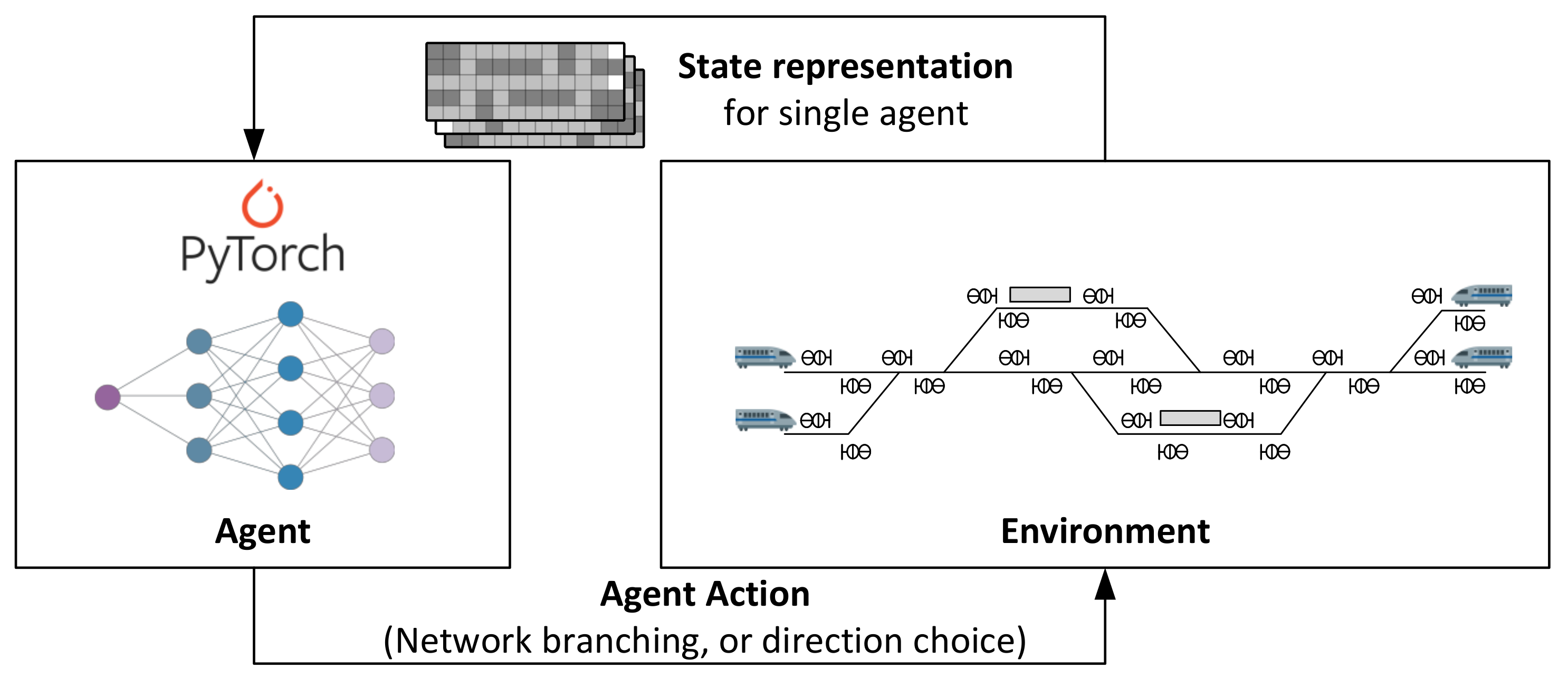
In multi-agent deep reinforcement learning, the framework changes from MDP to Markov games (MG), enabling the agents to interact with the shared environment and with each other. Thanks to that, additional challenges make the training even more difficult. The most crucial one is non-stationary, where the transition probability function changes. The utilized approach in our research is the independent learner concept, where the shared function approximator decides for only one agent at a time. Consequently, the state representation is composed in a manner where the other agents are handled as part of the environment from the current self-agent standpoint.
Figure 1 shows the training loop for the MADRL approach. Other MADRL methods exist that decide for all the agents at once. This is called centralized control. However, centralized MADRL methods cannot be robust to the change number of agents since they would change the output dimension of the used function approximator. Furthermore, the increase in the action space size also causes struggle during the algorithm’s training, which can be clearly observed on the convergence plots. Consequently, we utilized the independent learner concept, which limits the size of the action space, supports convergence, and is invariant to the change in the number of agents.
Deep Q-Network
The utilized DRL algorithm is the value-based deep Q-network (DQN). The DQN algorithm reached the first significant results that started to spread DRL as a methodology that can be used for solving complex sequential decision-making problems [
26]. This approach trains a neural network to predict the state–action value of every action in every given state as precisely as possible. These values can be considered to be a situation interpretation since they do not suggest choosing any of the actions directly, just exposing their worth in the long run. For training purposes, the target value that makes it possible to calculate the loss function is calculated with the Bellman equation:
where
is the given state in time step
t and
is the chosen action in time step
t.
is the discount factor,
represents the weights of the neural network, and
stands for the weights of the target neural network. While
is the reward provided by the environment in time step
.
2.2. Monte Carlo Tree Search
Monte Carlo tree search has earned the researchers’ consideration thanks to its fascinating results in a wild variety of challenging domains such as real-time strategy games (RTS) [
28], general video game playing (GVGP) [
29], and autonomous driving [
30]. Compared to other search-based methods such as uninformed approaches, MCTS can mitigate the required computational needs and provide guarantees that purely heuristic-based methods cannot. The component that distinguishes MCTS from other methods is the upper confidence bound for trees (UCT) algorithm proposed by [
31] that handles the exploration–exploitation trade-off inside the tree during the iteration process. The MCTS algorithm builds the tree-based form of the control problem with the help of the generative model of the environment; hence it is utilized as a model-based planner. Every iteration during the building of the tree uses four phases, which are the following:
Selection: Starting from the current root node, the algorithm recursively selects the child node on every branch with the highest UCT value until a leaf node occurs.
Expand: This phase encounters whether the leaf node found during selection is not terminal and child nodes can be populated from it. In that case, the algorithm populates the child nodes with the possible actions.
Simulation: This phase provides the first value assigned to a leaf node. To do so, it conducts a Monte Carlo rollout from the given leaf node until a terminal state of the environment encounters and assigns the value of the terminal state to the leaf node.
Backpropagation: In this final phase, the assigned state-value is backpropagated along the path traveled during the selection phase from root to leaf.
The above-mentioned UCT algorithm looks as follows:
where the exploration–exploitation trade-off is controlled via
called the temperature parameter,
is the visit count of the parent node,
is the visit count of the given node, and
is the given node’s average value. Another important advantage of the MCTS algorithm over its alternatives is that if enough iteration is given, then it can provide the globally optimal solution [
31].
During operating, the algorithm builds a search tree with the help of the four phases. The depth of the tree, hence the horizon, is determined by the provided number of iterations. After reaching the iterations, the information gathered inside the tree is utilized in the root node’s state. A policy has to be chosen beforehand to exploit the knowledge inside the children of the root node. The utilized policy, in this case, is the robust-child approach that chooses the action that populates the child node that has the most visit count compared to the other children. It is also important to mention that one decision only determines the next step of one train on the network. Consequently, the number of trains in the network determines how many layers in the tree belong to the same round where every train gets its
i-th action. For a more comprehensive study on MCTS, see [
32].
3. Environment
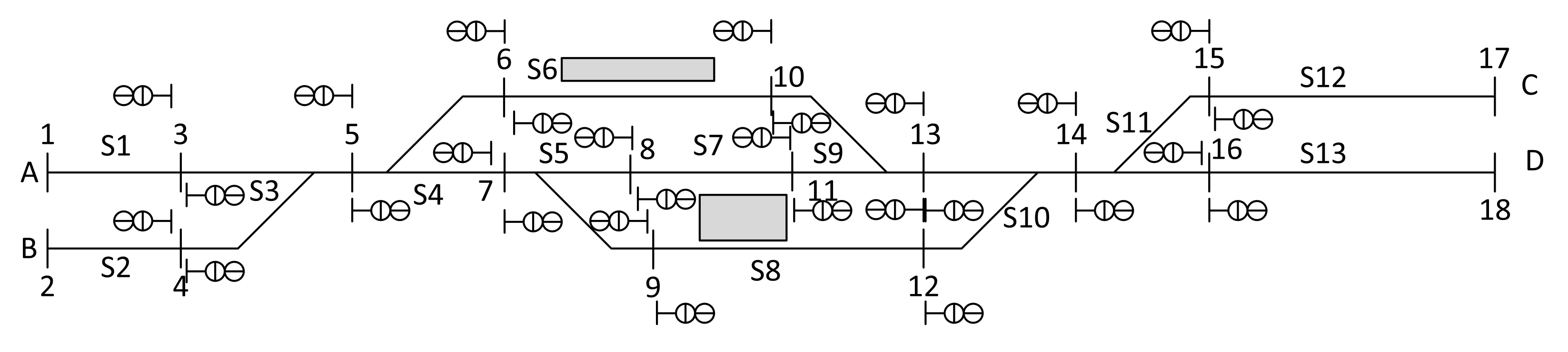
The description of the railway infrastructure is very complex, and hence it contains many different data fields, such as length of the section, the radius of the curve, the gradient of the track section, permitted speed for different train categories, etc. In the case of the trains—besides length—their acceleration, deceleration capability is essential. To solve the optimization, we need to select the minimum data required. Another problem is the decision-making process. Implementing all railway safety rules is hard because they cause problems since the environment did not learn the false actions. Initially, a directed graph-based description is used that contains the connections between vertices. A section between two or three vertices is called a track circuit or block section in the infrastructure. A section with three vertices is a switch, where the direction selection is possible. Traffic on the railway switch is direction dependent; only the trains coming from the facing point may choose the direction. It means that during the decision-making process, the traffic direction of the train is essential. The authors will present a simplified solution for this problem in this paper. An origin–destination (OD) matrix shown in
Table 1 describes the infrastructure represented in
Figure 2.
The OD matrix is a sheet-shaped representation of the infrastructure described by a directed graph. The nodes represent the limits of the track circuits, which can contain signals for one or both directions. The positive or negative signs of the cost values show the direction. Generally, the cost value can vary based on the gradient, maximum allowed speed, acceleration time, deceleration time, and temporary speed restrictions. In the reality, it is not constant and can vary depending on the traffic situation. This value cannot be zero, if there is a connection between two nodes. Zero means no possible route between signals. Directivity is essential when looking for a solution because the trains also can run in a positive or negative direction. This solution solves the problem of switches not finding forbidden nodes. In this paper, the cost value is proportional to the length, gradient and maximum allowed speed. The dimension of this value is [seconds]. The acceleration and deceleration times are zero, trains can run at maximum or zero speed. The direction is positive toward the entry/exit points C or D, negative otherwise. The model includes 13 track circuits (with sign S)— the value of the entry/exit track circuits is unit—and 18 decision-making points (vertices) represented by (virtual) signals in the reality. One track circuit may be busy for one train at a given time. Decision-making possibilities are waiting at the signal, continuing the journey toward one direction, or continuing the journey toward the second direction (if possible). Based on this model, state representation is possible.
3.1. Anomaly Detection in the Network
In an OCC, time-distance diagrams display the pre-planned timetable and the realized timetable to operators in real time. Based on the track vacancy data, the supervision system updates regularly the actual traffic situation in the HMI. The pre-planned schedule is a graph for each train. Based on the operational data, the information system draws the realized graph and tries to estimate the future traffic situation. The database of conflicted zones—single track sections, switching zones, following trains—is static data implemented in the information system. The pre-planned timetable contains the pre-planned route order of each train (and other necessary data, such as planned arrival, departure time, etc.). Due to the actual and planned schedule, the route conflicts appear—well in advance—in the time–distance diagram in real time. In some cases, a delay of a train does not lead to route conflict. It is a deviation from the timetable but does not requires rescheduling or reordering task performed by the dispatcher. If the planned timetable—based on the actual data—leads to a route conflict, it is a disturbance. It is necessary to alert the dispatcher visually through the time–distance diagram.
The automatic route setting system (ARS) gives route setting orders based on the planned data. The interlocking system does not perform the route setting orders—coming from the ARS—in the case of a conflicted situation to not lead to a traffic violation. The advanced scheduling systems recognize these situations early and alert the operators.
At this time, the dispatcher may take corrective measures. The operator can reorder and reschedule the affected trains.
3.2. State Representation
State representation is a crucial aspect of RL since this is the only information that an agent has for understanding the control problem. Consequently, it has to contain all the influential features of the domain in a manner that is also straightforward and sufficiently supports credit assignment. The composition of such solely depends on the researcher’s intuitions about the environment. Hence, this single component of the abstraction can profoundly influence the convergence and final performance.
3.2.1. Feature-Based Value Vector Representation
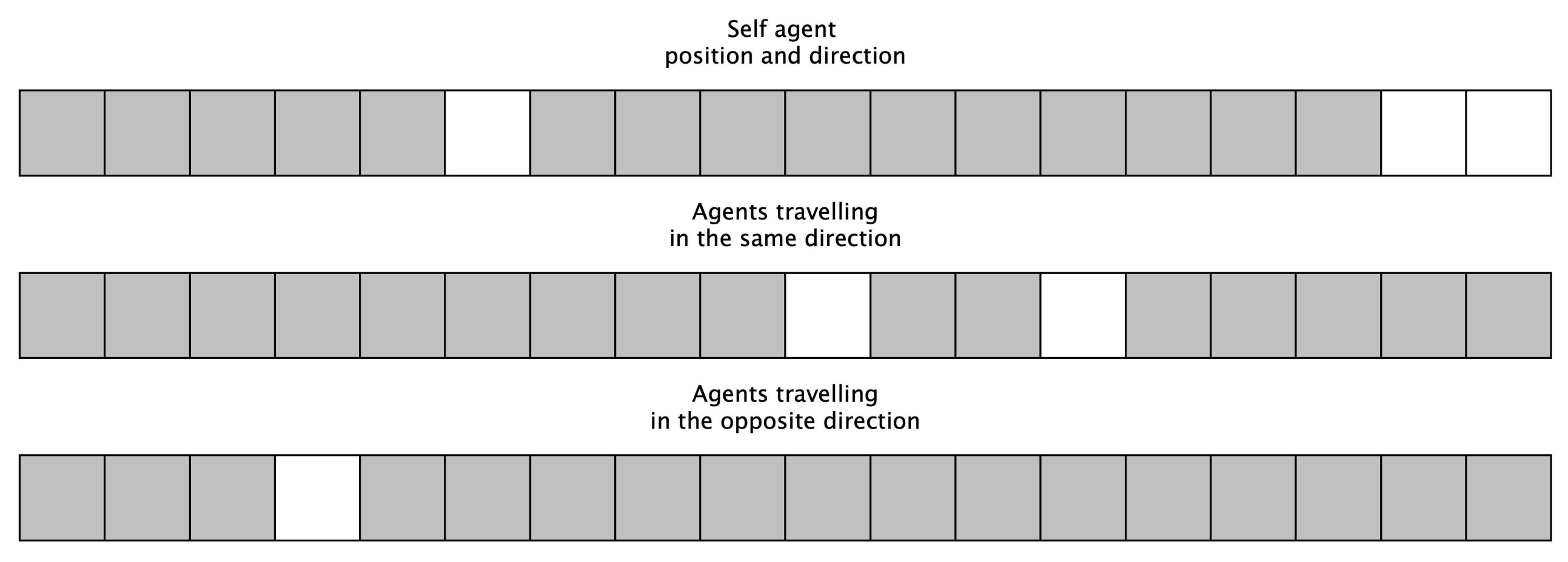
In this concept, every signal is interpreted as a decision-making point for the agent. The system’s map is composed so that every decision-making point is represented with one value that can be [0–1] based on their occupancy. As introduced in the methodology section, an independent learner MADRL approach is applied. Hence from the aspect of the agent in a given state, it only chooses an action for one train, while the other trains are considered as part of the environment. For that, the first component of the representation shows the current self-train position on the occupancy map combined with the goal positions, which are also represented with simple one-hot codes. With this approach, the position and direction of the self-train are given. However, in this domain, these two pieces of information of the other trains also have to be considered. From a strategic standpoint, it is essential to know which trains travel to the same and the opposite directions with the current self-train. Consequently, two more occupancy maps are created for the agent. The first one shows the trains that travel in the same direction, and the second shows the trains that go to the opposite. For clarity, we composed a loose representation with one-hot encoding on purpose, since in our previous endeavors, we experienced that it leads to better and quicker separation of the state–space, which profoundly affects the convergence of the utilized algorithm. The state representation is displayed in
Figure 3.
3.2.2. Image-like Representation
In the second approach, the network layout is modeled as a 2D grid-world, which is also one-hot encoded based on the cells’ occupancy and the walls that surround the free path of the network. In the formulation of the channels for the representation, we have the same concerns as in the feature-based case, notably, that the current decision maker should be aware of the other agents’ position and direction along with the required exit position. However, in this case, there is one more. In the feature-based case, the whole network is a directed graph where it is not allowed to move backward since it is impossible for a train to do so. Consequently, the actions only provide steps in the right direction. However, in the grid-world, the possible steps are the four direction. Hence, somehow, the agents have to be aware of the directed graph nature of the free path in a way that supports generalization. This problem is solved in the first channel.
Channel 1: In the first channel, the network’s layout is shown to the agent, where the walls are represented with ones and the free path with zeros. The directed graph nature of the network is represented to the agent by putting walls—ones—into the positions next to the agent, which would mean going in the reverse direction. This complement is consistent with the representation since there are walls surrounding the free paths and, thanks to that, supports generalization. Furthermore, it perfectly provides the necessary information about the directed nature of the problem.
Channel 2: This channel shows the position of the current decision maker in the network by setting the particular cell’s value to one, while every other cells’ value is set to zero.
Channel 3: This channel shows the goal position of the current decision maker in the network by setting the particular cell’s value to one, while every other cells’ value is set to zero.
Channel 4: This channel shows the position of all the other trains in the network that travels in the same direction as the current decision maker by setting their cells’ value to one. While every other cells’ value is set to zero.
Channel 5: This channel shows the position of all the other trains in the network that travels in the opposite direction as the current decision-maker by setting their cells’ value to one. While every other cells’ value is set to zero.
An example of the proposed image-like representation is shown in
Figure 4.
3.2.3. Flatland Global Observation
In the Flatland environment, there are two main approaches for state representation. In this paper, the image-like version is used for comparability. The utilized channels are the following.
Channel 1: The position and the travel direction of the current decision-maker are shown in this channel.
Channel 2: The position and travel direction of all other agents in the network are shown in this channel.
Channel 3: This channel encodes all the agents’ malfunctions in the network.
Channel 4: This channel provides information about the speed of all the agents in the network.
Channel 5: This channel shows the agents that are ready to depart from a station in the network.
Not all the channels are used since some do not apply to our version of the control problem. Consequently, only the first and second channels are used since these represent the strategic aspect of the problem altogether.
3.3. Action Space
The proper choice of action spaces crucially determines the level of generalization that can be reached during the training process. Furthermore, it is also essential to choose the action space in a manner that is consistent with the state representation. The primary approach is to formulate an action space where the individual actions carry the same meaning regardless of the given state. Of course, it is not possible in some cases. Still, if the concept ultimately lacks this virtue, then the agent has to learn the meaning of all the actions for every state, which is the exact opposite of generalization. This paper utilizes two different action spaces based on the introduced state representations.
3.3.1. Actions for Vector Based Representation
For the vector-based approach, the action space consists of three actions since, in our graph, every node has a maximum of two edges in a particular direction. The order between the actions is based on which one branches from the line that is considered the main one. Through that, it can be generalized over the network. From a strategic standpoint, the third action has an essential meaning in the control problem: waiting when a train remains in the given position. Thanks to that, deadlocks can be avoided.
3.3.2. Actions for Image-like Representation
In the image-like case, the choice of the action space is straightforward. It is the same as in any grid-world action for the four directions, complemented with the waiting action. This action space perfectly satisfies the previous statement about the state-invariant nature of the actions’ meaning.
3.4. Rewarding Concept
The last part of the abstraction is the rewarding strategy. Its primary role in the whole training process is to characterize the individual actions on the environment in a given scenario. Thanks to that, the agent can develop a desired behavior from the performance measures. Of course, the same difficulties go for the formulation of such a concept as in the case of the state representation, notably that the idea for such depends solely on the researcher’s intuition. However, it crucially affects the final performance. Furthermore, in MADRL, additional responsibility is given to the researchers’ since a trade-off between cooperation and competitiveness has to be formulated. In our case, the trade-off depends on the individual performance and whether the control problem is solved without conflicts. At the same time, the reward is presented for the agents only at the end of the episode. In every other case, the reward is zero, and it is also zero for every agent if a conflict occurs. The maximum reward is one, and its first portion is earned when the control problem is solved. The second portion is earned based on the agents’ individual performance, which is proportional to the steps taken for arriving into the goal position. Hence, the reward function looks as follows:
where
is the
i-th train’s performance-based reward calculated by considering the number of steps used for arriving in the desired position, while
is the reward component for solving the given scenario.
is the
i-th train’s episodic reward.
The minimization of the steps required for reaching the desired exit position is chosen as the basis of the rewarding concept. Since the number of steps represents the same meaning as the minimization of the journey time of the trains on the model’s level of abstraction.
4. Results
In this section, the different solutions are compared to evaluate their performance. For compatibility, the vector-based MADRL approach is compared with the search-based solution since their topology is the same. In contrast, the image-like representations are compared with each other because the number of steps is not representative compared with the other solutions. However, the basis for the comparison is the same, which is the number of steps required for solving the test episodes and the success rate that describes the frequency of solving the episodes without deadlock. The flexibility of the different image-like representations is demonstrated through training with both the original and mirrored network versions. Thanks to that, the generalization potential of the representation can be evaluated. Furthermore, both versions of the grid-world representation are trained to the different versions of the network separately to clarify the possible performance losses when they are trained for both simultaneously.
4.1. Training
In the training phase, every solution is treated in the same way. Notably, they have the same number of episodes to learn the control problem correctly. Every episode starts from a randomized initial state where the four trains are arbitrarily placed in the network and then assigned to a direction. Then the agents receive a fixed amount of steps to deliver all the trains to their exit points without any deadlocks. If an invalid action during this process causes a conflict or drives the agent into a wall, then the action is not executed, and the episodes will not be terminated. In our experience, we observed that this approach supports the training since it enables the agent to collect additional information in a possibly complex situation, making the memory pool more balanced.
Thanks to the topological differences, only the image-like representations are worth comparing in terms of the convergence of the algorithms. During the training process, all four approaches use the same random seeds, network structure, and hyperparameters for comparability.
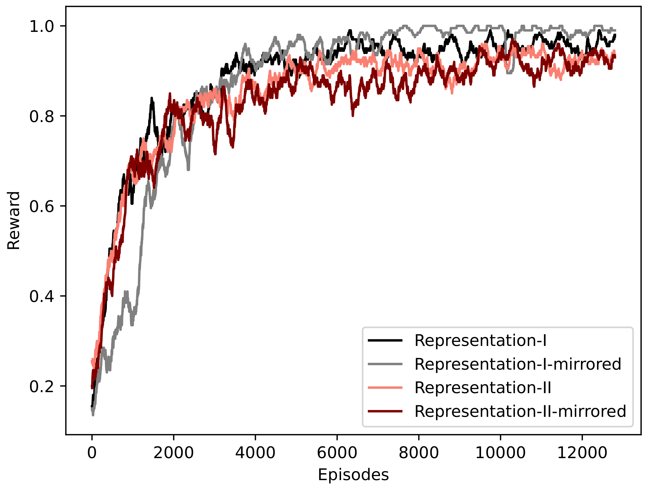
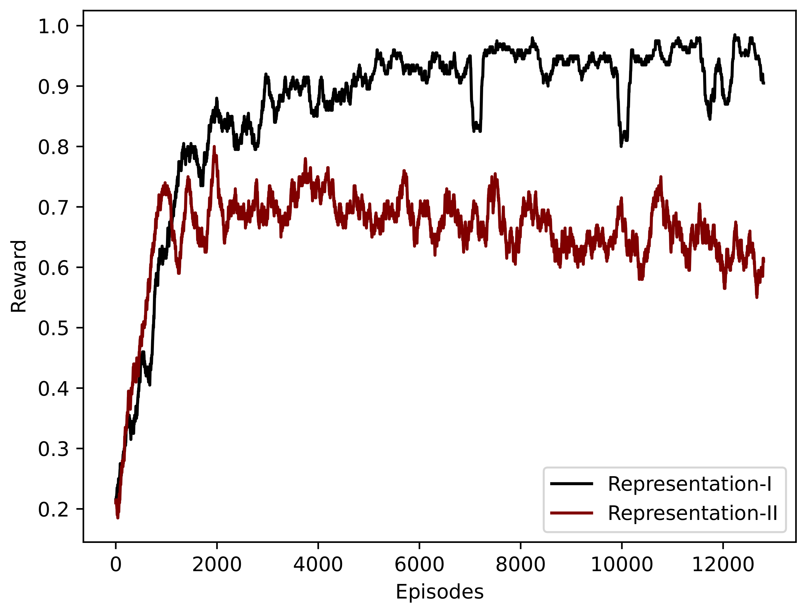
Figure 5 shows the convergence of both representations. Representation-I stands for the state representation proposed by this paper, while Representation-II is the state representation formulated based on the Flatland global observation. The
M letter determines whether the mirrored or the original network is utilized exclusively during training.
All the convergence graphs in
Figure 5 suggest that despite a small difference in stability and presumed final performance for the benefit of the proposed state representation, the different approaches can learn how to solve a single network.
However, training is conducted when the agents have to learn to solve the control problem in both the original and the mirrored network. In this training process, not just the initial positions of the trains are randomized, but the network layout itself.
Figure 6 shows the convergence of the two image-like representations for the case where the control problem has to be solved in both network layouts. In this case, the difference between the proposed and the Flatland representation is significant and predicts a significant discrepancy in the performance. Nevertheless, the proposed state representation sustains the characteristics of the previous case where only one network layout has to be learned, which shows the generalization potential in advance.
4.2. Comparison of MCTS and Vector-Based MADRL
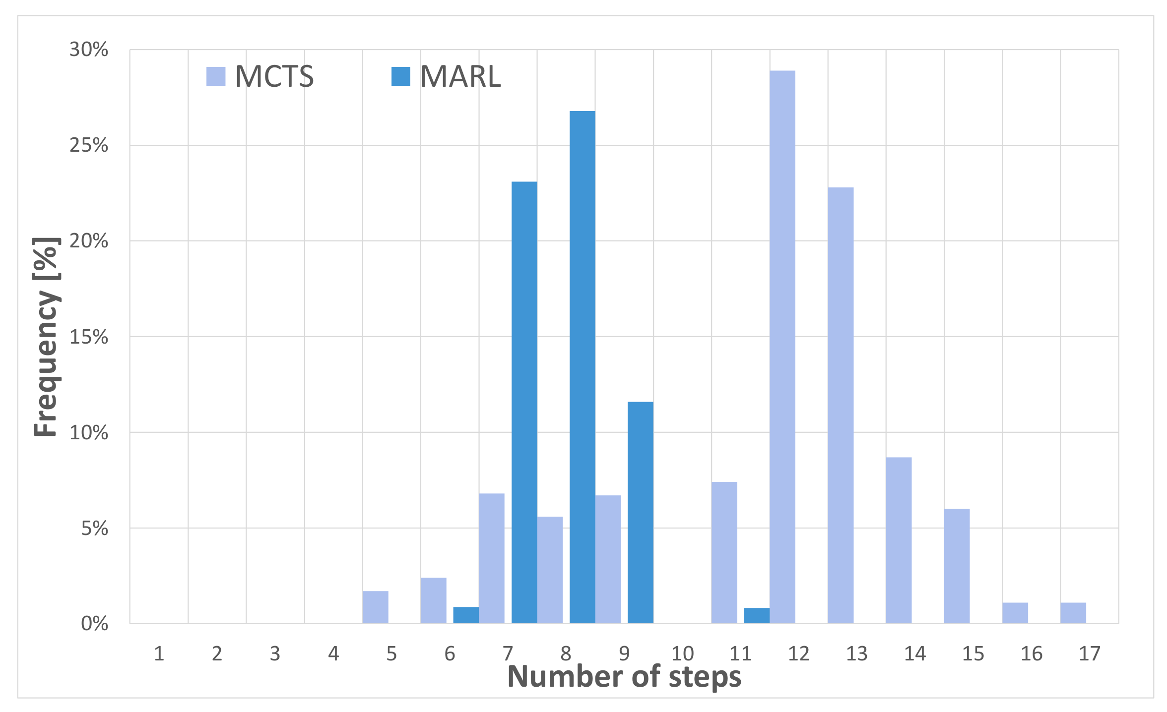
In the first part of the evaluation process, both the vector-based MADRL and the MCTS approaches are compared since these solutions share the same topology, which is the pledge of representativeness. The trains’ initial positions are randomly generated during evaluation. Of course, the random seeds are fixed for all one thousand episodes for both solutions to ensure comparability. The performance of the different solutions is measured based on the number of steps required for solving the test episodes.
Figure 7 shows the results of the comparison. Both the MADRL and MCTS algorithms solve all the episodes without any deadlocks, but the MADRL approach requires fewer steps, which is demonstrated by the higher frequencies in the left and middle portions of
Figure 7. Hence it provides better performance compared to MCTS. The reason for that is that the quality of the MCTS results is crucially affected by provided planning time. In that regard, a trade-off has to be made to mitigate the necessary computation time for making a single decision. Consequently, the core performance difference between the two solutions is the MCTS algorithm’s tremendous need for computational resources, which cannot be provided while real-time applicability is required. Furthermore, a straightforward formulation enables the absolute exploitation of the MADRL method’s potential.
4.3. Comparison of the Image-like Representations
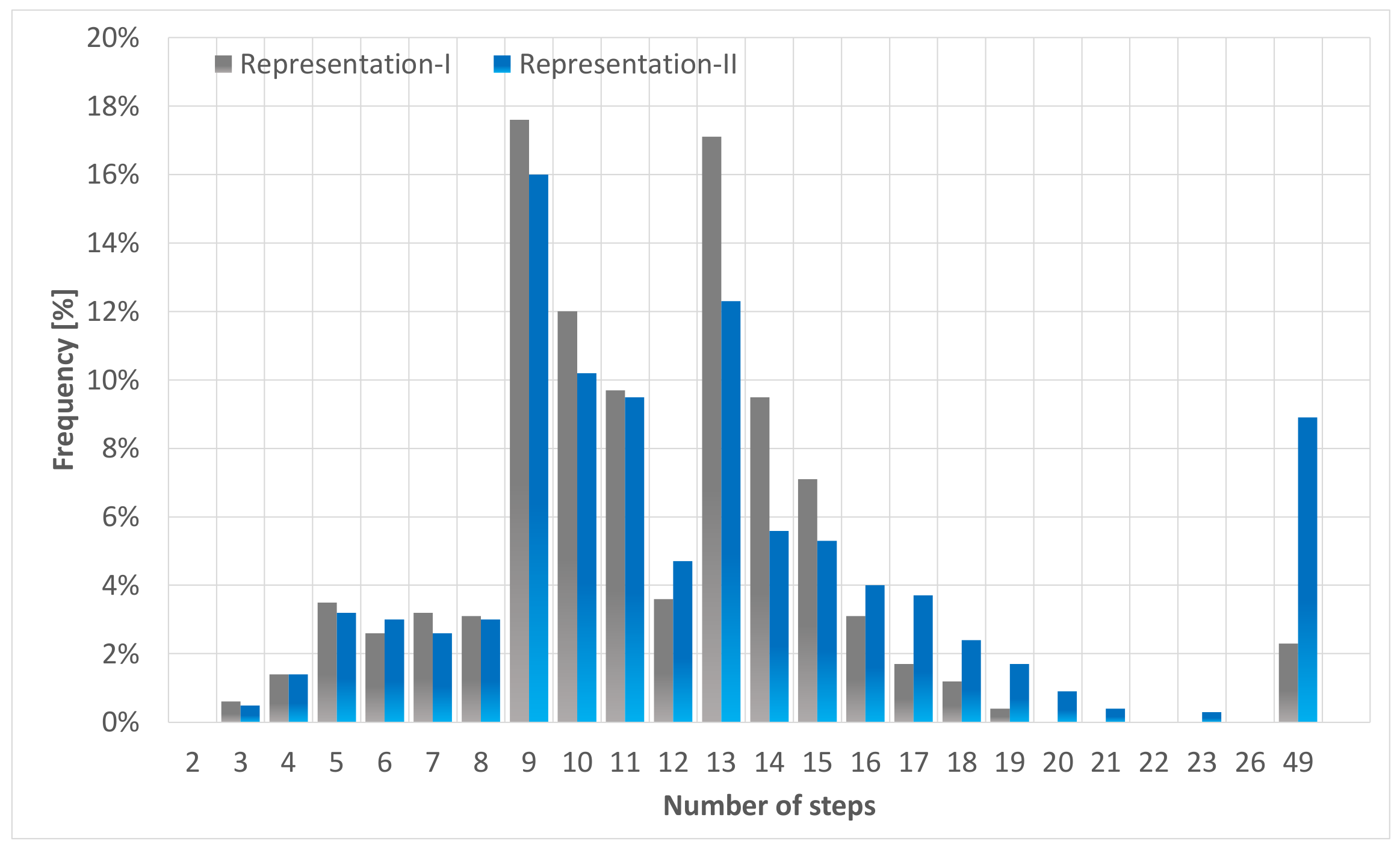
The image-like representations are compared in the same manner as mentioned above. Hence on the same one thousand episodes with the same random seeds, consequently on the same test episodes. However, the evaluation is divided into three parts. In the first part, the versions trained for only the original network are evaluated. The performance in terms of the number of steps used for solving the test episodes is shown in
Figure 8. The proposed representation and the Flatland global observation reach a success rate higher than 90%. Still, our approach, trained with the same parameters, solves 6% more test episodes without deadlock than the Flatland global observation. Furthermore, by checking the left and middle areas of
Figure 8, it can be seen that our approach utilizes fever steps on average, hence providing a better solution for the control problem overall.
The second part compares the versions trained for the mirrored network layout. The characteristics of the results are nearly the same as the previous one. The comparison is shown in
Figure 9. Both solutions provide success rates above 90%, but our approach outperforms the Flatland global observation with approximately 2%, thus utilizing fewer steps for solving the test episodes. In the case of the image-like representation, the performance difference is not that significant when the agents only have to learn one network during the entire training process. However, the source definitely, through the additional channels in the proposed state representation that enable a better understanding of the control problem for the agents, has an improved performance.
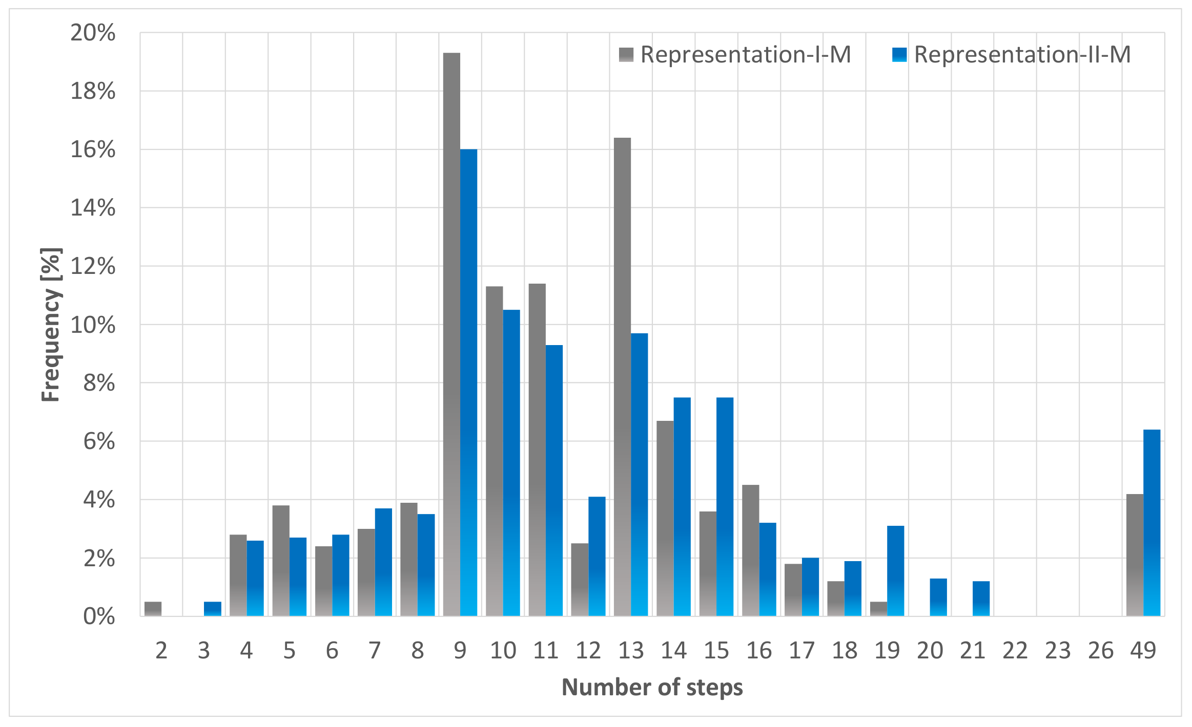
In the third part, the algorithms trained simultaneously for both network layouts are compared. The evaluation procedure is the same as in the previous cases. The performance discrepancy should be significant based on the convergence plot introduced above. The result is shown in
Figure 10. Comparing the characteristics of the proposed method that trained for both network layouts, it can be seen that it nearly reaches the same performance as in the case when exclusively trained for only one network type, which clearly demonstrates the potential for generalization. In the meantime, the Flatland global observation suffers a remarkable performance discrepancy compared to the cases when only trained for a sole network type. Compared to each other, the proposed representation maintains the success rate above 90%, while the other solutions struggle at approximately 60%. Moreover, when it solves the given test episodes, it utilizes a greater number of steps, thus providing an inferior performance compared to the proposed representation’s results. When the agents are trained for both the mirrored and the original network, the performance improvement of the proposed representation arises from the additional channel that clearly defines the network architecture. With this channel, the agent can understand the concept of the free path, and thanks to that, it can generalize through different layouts.
4.4. Understanding of the Results
The vector-based state representation shows excellent results; however, a trained model with this approach cannot be used for solving any other networks since it does not know anything about the network layout. It just learns the given one correctly, hence does not carry the potential for generalization. Still, the network infrastructure in the real world does not change too often. Consequently, the generalization potential is not the only aspect in the assessment since the safe and efficient control always carries significant value. Furthermore, if the particular network has changed, it can be easily retrained with the new layout. In the meantime, the MCTS algorithm is considered a general solution for such a problem. Still, more extensive network architectures will clearly lack the required computational needs, which prevents the algorithm from the real-time operation. On the contrary, the image-like representations significantly support generalization. The first component comes from the action space. Still, as the results showed, the Flatland global observation is not sufficient when learning more networks at once, not to mention further generalization tests, such as operating on a totally unknown network. In the meantime, the proposed method successfully solved the control problem on both network layouts simultaneously. The sole and most important reason for that is the layout channel in the representation, whose existence enables the agent to understand the concept of the free path. Through that, it does not overfit a single network but learns which paths can be used or not. Furthermore, the goal channel also allows learning how to navigate the network flexibly. With all these advances, the proposed network architecture, in theory, can be capable of solving any network layout. However, this approach also has limitations that arise from the fact that the image’s height and width predetermine the size of the network that can be represented in the given grid-world.
5. Conclusions
This paper presents three environment representation methods and three different solutions for solving the real-time railway rescheduling problem. The first is a MADRL-based approach with a vector-based stat representation compared with the MCTS algorithm utilized as a model-based planner. The comparison shows that both methods can solve all the test episodes without deadlock. However, the MCTS algorithm, thanks to its computational requirements, reaches weaker performance compared to MADRL. Unfortunately, the vector-based state representation does not carry significant generalization potential, mainly because it lacks understanding of the network layout concept. The action space that can be utilized in such a formulation of the control problem also brings difficulty in reaching suitable generalization. It requires learning the meaning of the actions in the different positions individually.
Consequently, an image-like representation is proposed that enables the agent to navigate on a layout to tackle these issues, not just to learn a particular network architecture, but to understand which paths can or cannot be used while driving a train from a given position to its desired exit point. A comparison is made between the interpretation of the Flatland global observation and the proposed state representation to demonstrate this potential. The results show that a channel that carries information about the network layout is necessary for acceptable generalization. However, this concept also has its limitations, notably that the network architectures size that can be used for learning and testing also is bounded by the frame size of the image used for training. We would like to focus on other limitations of the proposed representation in our future endeavors. Firstly, it cannot handle a sequence of connected networks, which would be an essential virtue. There are many lines where elementary networks are connected and have to be handled simultaneously to consider the neighboring networks. One can wonder that representing them in one picture is not advisable since the information density of the image would be more than worse. Secondly, it is also vital to further improve the complexity of the environment in terms of the dynamics of the trains to compare the results in measures, such as delays energy efficiency, that is meaningful for the railway industry. Thanks to the enormous safety concerns, testing and validating the performance of methods applied in the railway industry is crucial. Consequently, we are currently gathering data through a partnership with the Hungarian State Railways to further test and validate our solution in real-world networks and scenarios. In the following, we detail the possible workflow of our system that we would like to test in our further endeavors. The MADRL solution determines the exact route of each train. The new rescheduled/rerouted solution is available at the end of the algorithm. It determines the new conflict-free solution with the new route orders of each train. The first step to realizing the decision is to modify the planned timetable of each train in the time–distance diagram. In this case, the newly planned timetable contains the modified routes and the delays caused by the disturbance. The ARS system can perform the route setting orders in the next step. The transformation into the scheduling system is fast due to the advanced information systems (which means seconds). The transformation into the scheduling system is fast due to the advanced information systems (which means seconds). The exact route setting order from an OCC realizes the switching process and controls the signals. The average time of the realization of each route setting order is between 5 s and 30 s, depending on the number of points operated.
Author Contributions
Conceptualization, T.B. and S.A.; methodology, I.L. and B.K.; software, I.L. and B.K.; validation, T.B.; resources, S.A.; writing—original draft preparation, I.L. and B.K.; writing—review and editing, T.B. and S.A.; visualization, B.K. and T.B.; supervision, S.A. All authors have read and agreed to the published version of the manuscript.
Funding
The research reported in this paper is part of project no. BME-NVA-02, implemented with the support provided by the Ministry of Innovation and Technology of Hungary from the National Research, Development and Innovation Fund, financed under the TKP2021 funding scheme. The research was also supported by the Hungarian Government and co-financed by the European Social Fund through the project “Talent management in autonomous vehicle control technologies” (EFOP-3.6.3-VEKOP-16-2017-00001). This paper was also supported by the János Bolyai Research Scholarship of the Hungarian Academy of Sciences.
Institutional Review Board Statement
Not applicable.
Informed Consent Statement
Not applicable.
Data Availability Statement
Not applicable.
Conflicts of Interest
The authors declare no conflict of interest.
Abbreviations
The following abbreviations are used in this manuscript:
| ATC | Automatic Train Control |
| ATO | Automatic Train Operation |
| OCC | Operation Control Centers |
| ETCS | European Train Controlling System |
| RBC | Radio Block Center |
| ARS | Automated Route Setting System |
| ATP | Automatic Train Protection |
| ROMA | Railway Traffic Optimization by Means of Alternative Graphs |
| DIZ | Dynamic Impact Zone |
| CPS | Conflict Prevent Strategy |
| DQN | Deep Q-Network |
| DRL | Deep Reinforcement Learning |
| MADRL | Multi-Agent Deep Reinforcement Learning |
| MDP | Markov Decision Process |
| MG | Markov Games |
| MCTS | Monte Carlo Tree Search |
| GVGP | General Video Game Playing |
| RTS | Real-Time Strategy |
| UCT | Upper Confidence Bound for Trees |
| OD | Origin Destination |
| CNN | Convolutional Neural Network |
References
- European Commission. Sustainable and Smart Mobility Strategy—Putting European Transport on Track for the Future. 2021. Available online: https://transport.ec.europa.eu/system/files/2021-04/2021-mobility-strategy-and-action-plan.pdf (accessed on 7 January 2022).
- De Martinis, V.; Corman, F. Data-driven perspectives for energy efficient operations in railway systems: Current practices and future opportunities. Transp. Res. Part C Emerg. Technol. 2018, 95, 679–697. [Google Scholar] [CrossRef]
- Parvez Farazi, N.; Zou, B.; Ahamed, T.; Barua, L. Deep reinforcement learning in transportation research: A review. Transp. Res. Interdiscip. Perspect. 2021, 11, 100425. [Google Scholar] [CrossRef]
- Hansen, I.A.; Pachl, J. Railway Timetabling and Operations; Eurailpress, DVV Media Group GmbH: Hamburg, Germany, 2008; pp. 155–173. [Google Scholar]
- D’Ariano, A.; Albrecht, T. Running time re-optimization during real-time timetable perturbations. WIT Trans. State Art Sci. Eng. 2010, 40, 147–156. [Google Scholar] [CrossRef]
- Tan, Y.; Xu, W.; Jiang, Z.; Wang, Z.; Sun, B. Inserting extra train services on high-speed railway. Period. Polytech. Transp. Eng. 2021, 49, 16–24. [Google Scholar] [CrossRef] [Green Version]
- Mascis, A.; Pacciarelli, D. Job-shop scheduling with blocking and no-wait constraints. Eur. J. Oper. Res. 2002, 143, 498–517. [Google Scholar] [CrossRef]
- D’Ariano, A.; Corman, F.; Pacciarelli, D.; Pranzo, M. Reordering and local rerouting strategies to manage train traffic in real time. Transp. Sci. 2008, 42, 405–419. [Google Scholar] [CrossRef]
- Corman, F.; D’Ariano, A.; Pacciarelli, D.; Pranzo, M. A tabu search algorithm for rerouting trains during rail operations. Transp. Res. Part B Methodol. 2010, 44, 175–192. [Google Scholar] [CrossRef]
- Van Thielen, S.; Corman, F.; Vansteenwegen, P. Towards a conflict prevention strategy applicable for real-time railway traffic management. J. Rail Transp. Plan. Manag. 2019, 11, 100139. [Google Scholar] [CrossRef]
- Krasemann, J.T. Computational decision-support for railway traffic management and associated configuration challenges: An experimental study. J. Rail Transp. Plan. Manag. 2015, 5, 95–109. [Google Scholar] [CrossRef] [Green Version]
- Pellegrini, P.; Marlière, G.; Pesenti, R.; Rodriguez, J. RECIFE-MILP: An Effective MILP-Based Heuristic for the Real-Time Railway Traffic Management Problem. IEEE Trans. Intell. Transp. Syst. 2015, 16, 2609–2619. [Google Scholar] [CrossRef] [Green Version]
- Zhu, Y.; Goverde, R.M. Railway timetable rescheduling with flexible stopping and flexible short-turning during disruptions. Transp. Res. Part B Methodol. 2019, 123, 149–181. [Google Scholar] [CrossRef]
- Lindenmaier, L.; Lövétei, I.F.; Lukács, G.; Aradi, S. Infrastructure Modeling and Optimization to Solve Real-time Railway Traffic Management Problems. Period. Polytech. Transp. Eng. 2021, 49, 270–282. [Google Scholar] [CrossRef]
- Pellegrini, P.; Marlière, G.; Rodriguez, J. A detailed analysis of the actual impact of real-time railway traffic management optimization. J. Rail Transp. Plan. Manag. 2016, 6, 13–31. [Google Scholar] [CrossRef]
- Medeossi, G.; Nash, A. Reducing Delays on High-Density Railway Lines: London–Shenfield Case Study. Transp. Res. Rec. 2020, 2674, 193–205. [Google Scholar] [CrossRef]
- Luan, X.; Wang, Y.; De Schutter, B.; Meng, L.; Lodewijks, G.; Corman, F. Integration of real-time traffic management and train control for rail networks—Part 1: Optimization problems and solution approaches. Transp. Res. Part B Methodol. 2018, 115, 41–71. [Google Scholar] [CrossRef]
- D’Acierno, L.; Placido, A.; Botte, M.; Gallo, M.; Montella, B. Defining robust recovery solutions for preserving service quality during rail/metro systems failure. Int. J. Supply Oper. Manag. 2016, 3, 1351–1372. [Google Scholar]
- Botte, M.; Di Salvo, C.; Placido, A.; Montella, B.; D’Acierno, L. A Neighbourhood Search Algorithm for determining optimal intervention strategies in the case of metro system failures. Int. J. Transp. Dev. Integr. 2016, 1, 63–73. [Google Scholar] [CrossRef] [Green Version]
- Botte, M.; D’Acierno, L. Dispatching and rescheduling tasks and their interactions with travel demand and the energy domain: Models and algorithms. Urban Rail Transit 2018, 4, 163–197. [Google Scholar] [CrossRef]
- Lövétei, I.F.; Kővári, B.; Bécsi, T. MCTS Based Approach for Solvong Real-time Railway Rescheduling Problem. Period. Polytech. Transp. Eng. 2021, 49, 283–291. [Google Scholar] [CrossRef]
- Mohanty, S.; Nygren, E.; Laurent, F.; Schneider, M.; Scheller, C.; Bhattacharya, N.; Watson, J.; Egli, A.; Eichenberger, C.; Baumberger, C.; et al. Flatland-RL : Multi-Agent Reinforcement Learning on Trains. arXiv 2020, arXiv:2012.05893. [Google Scholar]
- Ning, L.; Li, Y.; Zhou, M.; Song, H.; Dong, H. A Deep Reinforcement Learning Approach to High-speed Train Timetable Rescheduling under Disturbances. In Proceedings of the 2019 IEEE Intelligent Transportation Systems Conference (ITSC), Auckland, New Zealand, 27–30 October 2019; pp. 3469–3474. [Google Scholar] [CrossRef]
- Obara, M.; Kashiyama, T.; Sekimoto, Y. Deep Reinforcement Learning Approach for Train Rescheduling Utilizing Graph Theory. In Proceedings of the 2018 IEEE International Conference on Big Data (Big Data), Seattle, WA, USA, 10–13 December 2018; pp. 4525–4533. [Google Scholar] [CrossRef]
- Yang, G.; Zhang, F.; Gong, C.; Zhang, S. Application of a Deep Deterministic Policy Gradient Algorithm for Energy-Aimed Timetable Rescheduling Problem. Energies 2019, 12, 3461. [Google Scholar] [CrossRef] [Green Version]
- Mnih, V.; Kavukcuoglu, K.; Silver, D.; Rusu, A.A.; Veness, J.; Bellemare, M.G.; Graves, A.; Riedmiller, M.; Fidjeland, A.K.; Ostrovski, G.; et al. Human-level control through deep reinforcement learning. Nature 2015, 518, 529–533. [Google Scholar] [CrossRef] [PubMed]
- Silver, D.; Schrittwieser, J.; Simonyan, K.; Antonoglou, I.; Huang, A.; Guez, A.; Hubert, T.; Baker, L.; Lai, M.; Bolton, A.; et al. Mastering the game of go without human knowledge. Nature 2017, 550, 354–359. [Google Scholar] [CrossRef] [PubMed]
- Farooq, S.S.; Oh, I.S.; Kim, M.J.; Kim, K.J. StarCraft AI competition report. AI Mag. 2016, 37, 102–107. [Google Scholar] [CrossRef] [Green Version]
- Perez, D.; Samothrakis, S.; Lucas, S. Knowledge-based fast evolutionary MCTS for general video game playing. In Proceedings of the 2014 IEEE Conference on Computational Intelligence and Games, Dortmund, Germany, 26–29 August 2014; pp. 1–8. [Google Scholar]
- Kovári, B.; Hegedüs, F.; Bécsi, T. Design of a Reinforcement Learning-Based Lane Keeping Planning Agent for Automated Vehicles. Appl. Sci. 2020, 10, 7171. [Google Scholar] [CrossRef]
- Kocsis, L.; Szepesvári, C. Bandit based monte-carlo planning. In European Conference on Machine Learning; Springer: Berlin/Heidelberg, Germany, 2006; pp. 282–293. [Google Scholar]
- Browne, C.B.; Powley, E.; Whitehouse, D.; Lucas, S.M.; Cowling, P.I.; Rohlfshagen, P.; Tavener, S.; Perez, D.; Samothrakis, S.; Colton, S. A survey of monte carlo tree search methods. IEEE Trans. Comput. Intell. AI Games 2012, 4, 1–43. [Google Scholar] [CrossRef] [Green Version]
| Publisher’s Note: MDPI stays neutral with regard to jurisdictional claims in published maps and institutional affiliations. |
© 2022 by the authors. Licensee MDPI, Basel, Switzerland. This article is an open access article distributed under the terms and conditions of the Creative Commons Attribution (CC BY) license (https://creativecommons.org/licenses/by/4.0/).


