Meteorological Conditions That Promote Persistent Contrails

Abstract

Climate-impacting contrails need ice (super-)saturation to persist longer than a few minutes. However, this simple criterion cannot be easily applied for the prediction of persistent contrails. The current weather forecast models, which lack humidity data for assimilation in the upper troposphere, have difficulties coping with the enormous variability and sharp gradients in the relative humidity field. Thus, ice supersaturation, which is an extremal state of relative humidity, is hard to forecast at a precise location and time to allow contrail-avoiding flight routing. In this paper, we investigate the possibility of using dynamical proxy variables for improved contrail prediction. This idea is guided by the fact that the probability of ice supersaturation differs in different dynamical regimes. Therefore, we determine probability distributions of temperature, water vapour concentration, vertical velocity, divergence, relative and potential vorticity, geopotential height, and lapse rate conditioned on three situations: (a) contrail persistence not possible; (b) contrail persistence possible; and (c) strongly warming persistent contrails possible. While the atmospheric variables are taken from reanalysis data, the conditions (a–c) are based on airborne measurement data and radiation quantities from the reanalysis. It turns out that the vorticity variables, and in particular geopotential and lapse rate, show quite distinct conditional probabilities, suggesting a possibility to base an improved forecast of persistent contrails not only on the traditional quantities of temperature and relative humidity, but on these dynamical proxies as well. Furthermore, we show the existence of long flight tracks with the formation of strongly warming contrails, which are probably embedded in larger ice-supersaturated regions with conditions that foster such contrails. For forecasting purposes, this is a beneficial property since the humidity forecast is easier on large, rather than small, spatial scales.

1. Introduction

Aviation contributes to climate change not only by its emission of CO${}_2$ but also by a number of non-CO${}_2$ effects, of which contrails and contrail cirrus are the only visible effect and also the most important one [1]. As aviation, despite the current depression caused by the pandemic, is a strongly growing sector, measures are needed to reduce its climate impact. One such measure is the avoidance of warming persistent contrails. In theory, forecasting persistent contrails is an easy task: predict where contrails form (Schmidt-Appleman criterion, see [2]) and where the relative humidity exceeds ice saturation (ice-supersaturated regions, ISSRs, see [3]). Unfortunately, in practice, it turns out that while the first step, the prediction of contrail formation, is moderately successful, the second, the prediction of persistence, is not good enough for a flight routing purpose that intends to avoid persistent contrails [4]. Even in cases where the whole sky is filled with persistent contrails, as on 21 September 2011 over the Gulf of Lion, numerical weather models indicate high but insufficient relative humidity below ice saturation [5].

The feature that makes forecasts of ice supersaturation difficult is the immense variability of the humidity field, temporally and spatially, with sharp gradients, as a glance to an arbitrary satellite image taken with the infrared water-vapour channel proves. Water vapour is involved in aerosol and chemical processes. It undergoes phase transformations, which depend on local dynamics (vertical motions causing adiabatic cooling and heating). Relative humidity is affected by changes of vapour concentration and temperature. All these processes, acting on many scales, contribute to the vast variability of the relative humidity field. Moreover, supersaturation is an extremal state that is more sensitive to synoptic, regional, and local conditions than mean humidity states. However, the situation is not hopeless since ice supersaturation does occur with different frequency or probability in different dynamic circumstances, see e.g., [6,7]. Thus, exploiting dynamical variables and the fact that ISSRs prefer certain regimes over others, can help to improve the forecast of contrail persistence.

This paper describes a study that is similar to [7], in that it shows probability distributions for situations where persistent contrails are possible or not (conditional distributions). However, we go further than [7] in several respects: (1) in addition to vertical velocity, divergence, and relative vorticity, we consider more dynamical fields; (2) instead of 4 months, we use 10 years of data, from 2000–2009, for a large fraction of the northern mid-latitudes; and (3) we use two independent data sets, being temperature and humidity, from airborne measurements as an independent truth (i.e., to determine whether persistent contrails are possible or not), and we use ERA-5 dynamical data at the same locations and times to study the dynamical variables. In contrast, ref. [7] used all data from the reanalysis.

In this paper, we not only consider whether a persistent contrail is possible or not, but we distinguish persistent contrails with a particularly large value of instantaneous radiative forcing, iRF. For this purpose, we use iRF data from [8], in the following abbreviated as WGR21]. The idea is to see whether an additional condition, namely “particularly large iRF”, may affect the derived probability distributions in a way that makes it possible to mainly concentrate the aspiration of contrail avoidance to these strong cases. Such a mitigation strategy, if it can be successfully implemented, would yield a considerable climate benefit at very low additional fuel burn and costs, and it would be more reliable and robust to deal with strong contrails instead of contrails with a small and perhaps uncertain radiative effect.

In the present paper, we first introduce our data sources and the methods that we apply (Section 2). Next, we present the statistical results (Section 3.1 and Section 3.2), that is, conditional distributions. Furthermore, we analyse how coherently in space strong values of iRF appear (Section 3.3) because avoidance of warming contrails will probably be facilitated if large iRF values occur in longer series and not intermittently. A discussion of the relation of iRF and the proper measure for the climate impact of an individual contrail follows in Section 3.4. A summary of the results is given in the final Section, together with conclusions and an outlook on further possibilities for contrail prediction.

2. Data and Methods

Essentially, the same sample of data is used in the present paper as in the former paper by the same authors (WGR21). Therefore, it suffices to simply mention these data without giving much detail. We will provide more detail only where we use additional data.

2.1. IAGOS/MOZAIC Data

The same temperature and relative humidity data are used as in WGR21, namely ten years (2000–2009) of data from the Measurement of Ozone and Water Vapour on Airbus In-service Aircraft (MOZAIC) program [9], which was, in 2011, transferred into the new European Research Infrastructure In-service Aircraft for a Global Observing System [IAGOS] [10]. The selected data from 16,588 flights refer to the northern midlatitude band from 30${}^{°}$ to 70${}^{°}$ latitude and $-{125}^{°}$ to 145${}^{°}$ longitude and to cruise levels between 310 and 190 hPa. These data are used to establish an independent “truth”; they are used to determine whether the formation of a persistent contrail was possible or not at the time and position of the respective measuring aircraft. Furthermore, they are used together with radiation quantities from the reanalysis data set to estimate instantaneous radiative forcing (iRF) values at those positions where persistent contrails are possible, see below.

2.2. ERA-5 Data

For each selected aircraft position and time in the IAGOS/MOZAIC data set, the corresponding weather data from ECMWF’s (European Centre for Medium-Range Weather Forecast) ERA-5 reanalysis [11,12,13] is retrieved and interpolated to the exact position and time. These data have been obtained in hourly resolution from the Copernicus Data Service [14]. Apart from the three radiation quantities and specific cloud ice-water content as in WGR21, to determine the iRF values, we retrieve the following thermodynamic and dynamic variables for pressure levels of 200, 225, 250, and 300 hPa: temperature, relative and absolute humidity, vertical velocity, divergence, relative vorticity, potential vorticity, and geopotential. Using pressure and temperatures on two adjacent levels, we later estimate a local lapse rate at the aircraft positions. The pressure range of 300 to 200 hPa covers approximately the flight levels of 300 to 390 hft.

2.3. Instantaneous Radiative Forcing

The instantaneous radiative forcing (iRF) is the difference in radiation flux at the top of the atmosphere in two situations, one with a contrail and the other without the contrail, but otherwise equal. To calculate this quantity, we assume that all contrails are 500 m high and that their ice crystals have an effective radius of 30 µm. Furthermore, we assume that all humidity in excess of ice saturation is converted to ice. For nearby and overlying cirrus, we assume a thickness of 1500 m and an effective radius of 60 µm. With these assumptions, we estimate the optical thickness of contrails and cirrus and then use the parameterization by [15] to compute iRF. For more details, we refer to WGR21. Here, we define contrails with an iRF exceeding 19 W m${}^{-2}$ as particularly strong cases. The value 19 W m${}^{-2}$ has no special significance. It is just about the mean iRF plus one standard deviation from WGR21.

2.4. Normalised Geopotential and Estimation of Lapse Rates

In this section, we explain the normalisation procedure for geopotential. The geopotential height increases with decreasing pressure. If one wants to determine conditional distributions of geopotential height under different conditions, either this has to be done for each pressure level separately or one finds a way to normalize its value by a prescribed standard geopotential height for each pressure level. Such a standardisation is possible as follows: Using a mean tropospheric temperature, $\overline{T}=255$ K, we determine a corresponding mean pressure scale height, $\overline{H}=R_d\overline{T}/g=7452$ m, with the gas constant for dry air, $R_d$, and the gravitational acceleration, g, (which we simply assume constant). We then define standard geopotential heights:

$$Z^{*}\left(p\right)=\overline{H}ln(p_s/p).$$

(1)

Here, the reference pressure $p_s=1000$ hPa, and p is one of the selected pressure levels. The resulting values are $Z^{*}(300,250,225,200\mathrm{hPa})$ = (8972, 10,331, 11,116, 11,994) m. Normalisation of Z with the appropriate $Z^{*}\left(p\right)$ results in unified ranges of about $0.9$ to $1.1$ for each level. Obviously, pressure levels vary quite considerably in altitude; the isobar at a nominal height of 10 km may actually vary between 9 and 11 km.

Furthermore, we analyse conditional distributions for the lapse rate, i.e., $\gamma =-\mathrm{d}T/\mathrm{d}z$. The procedure to estimate the lapse rate at the position of an aircraft is provided in a recent paper [16]. Hence, it suffices to give the final formula:

$$\gamma =\frac{g}{R_d}\frac{ln(T_0/T_1)}{ln(p_0/p_1)},$$

(2)

where the $(T_0,p_0)$ are the temperature and pressure of the nearest pressure level below the flight position, respectively, and $(T_1,p_1)$ are the corresponding values on the closest level above that point. Note that the lapse rate cannot be estimated for flight positions at 300 hPa or below, nor at 200 hPa and above, since only the data at the four pressure levels from 300 to 200 hPa are used in the analysis.

2.5. Determination of Probability Density Functions

For each quantity, we collect all data and sort them numerically. From this sorted list, we determine the cumulative distributions. The corresponding probability density functions, which are the derivatives of the cumulative distributions, are determined by employing a kernel density estimator (Epanechnikov kernel, see e.g., [17]). The optimal bin sizes were calculated by the program itself.

3. Results and Discussion

3.1. Temperature and Humidity Fields

This chapter will compare distributions of thermodynamic variables for conditions where persistent contrails, persistent contrails with particularly large iRF, and non-persistent contrails (or no contrails) occur. “Particularly large iRF” means that iRF exceeds the ten-years average plus one standard deviation, which gives iRF $\ge 19$ W m${}^{-2}$. Contrails were distinguished according to MOZAIC data, such that the Schmidt-Appleman quantities $R{H}_{\max }$ and $R{H}_i$ from the individual flight points decided whether a persistent contrail was possible. Here, $R{H}_{\max }$ is the relative humidity (with respect to liquid water) that the mixture of exhaust gases with ambient air transiently attains at the moment when its temperature reaches the threshold for contrail formation. $R{H}_{\max }$ must exceed unity for contrail formation to be possible (for the definition, see [4]). $R{H}_i$, the ambient relative humidity with respect to ice must exceed unity to allow contrail persistence. The distributions are given as probability density functions (pdf) that were produced with a kernel density estimator.

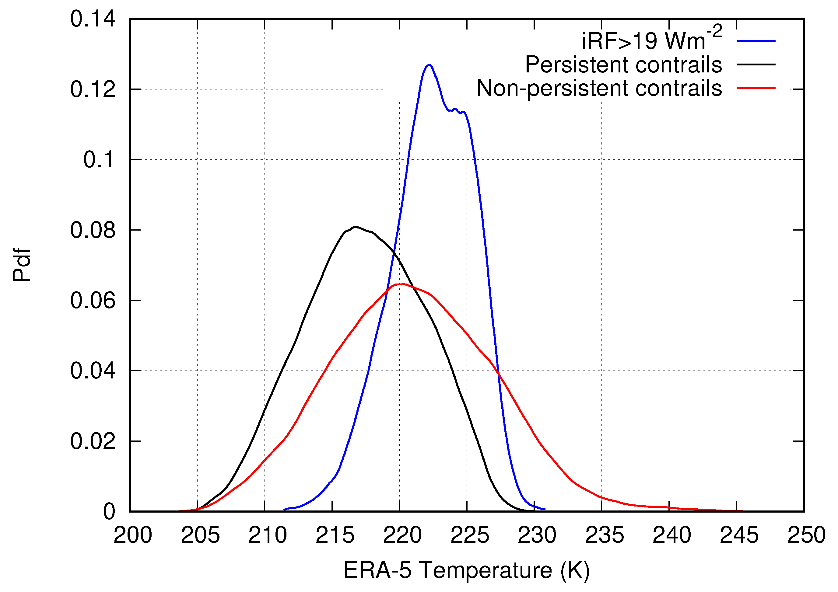
Figure 1 shows temperature distributions for the general situation (red, 390,486 cases), in situations that allow persistent contrails (black, 47032 cases), and in situations with large iRF (blue, 4052 cases). The pdfs show the temperatures from the ERA-5 reanalysis interpolated to the respective flight points from MOZAIC; however, the deciding factor for persistence (for all plots) are MOZAIC’s thermodynamic quantities. Only minimal differences between the temperature distributions of MOZAIC and ERA-5 are observed (not shown), indicating that ERA-5 predicts temperatures for the flight points from MOZAIC well. MOZAIC aircraft fly at temperatures between 200 and 250 K. Persistent contrails occur at the lower end of the distribution, and the Schmidt-Appleman threshold sets an upper limit for situations with contrails at about 230 K. Contrails with large iRF occur predominantly at temperatures a few degrees (say, 3 to 8 K) below the threshold, but not at the lowest temperatures that persistent contrails in our data attain. This is explained by the fact that absolute humidity generally increases with temperature, such that more ice can form and higher contrail optical thickness can be reached at higher temperatures, not too far below the contrail formation threshold. 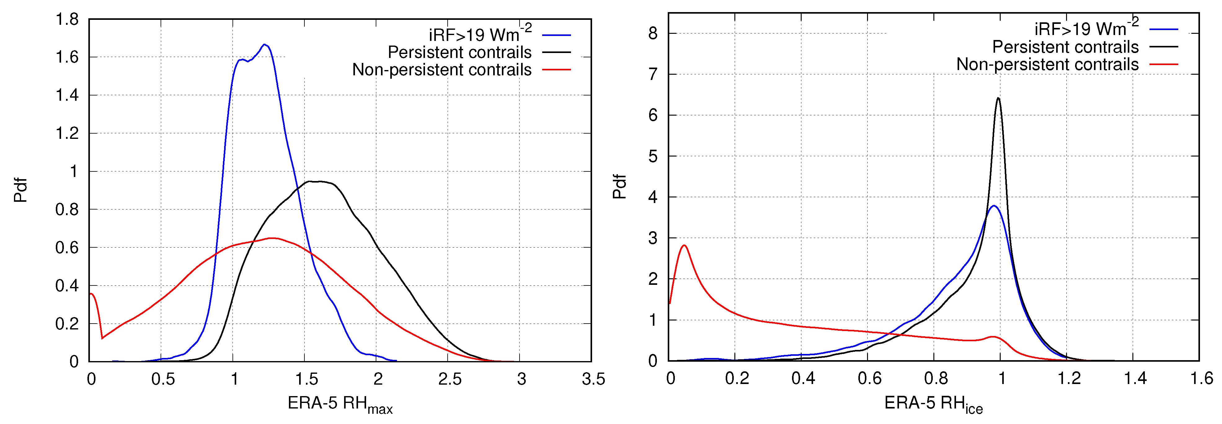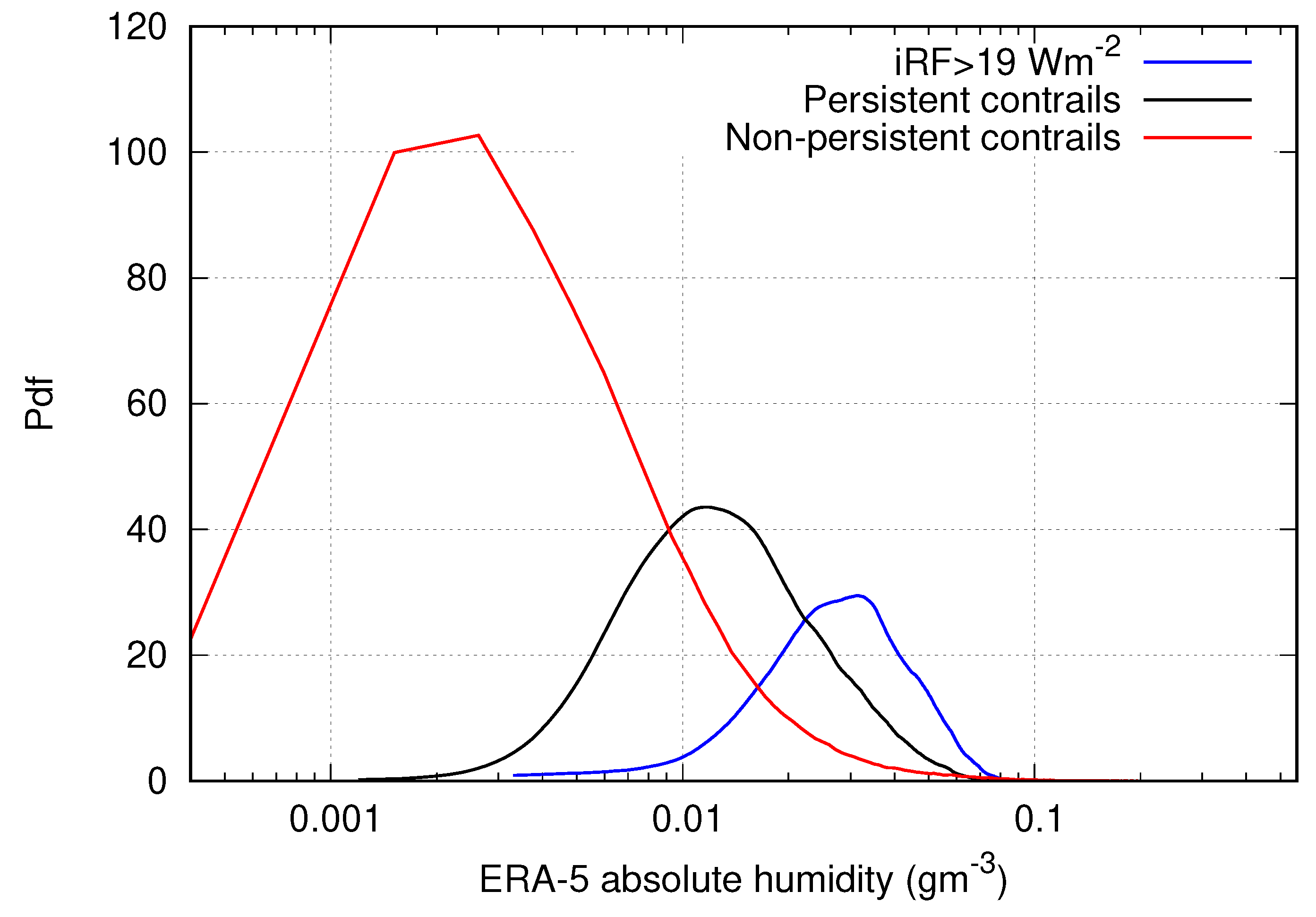Figure 2 confirms that contrails with large iRF particularly develop at the highest absolute humidities, as the pdf for this condition (blue line) is shifted relative to that for persistent contrails in general (black line) towards higher values.

In Figure 3, pdfs for $R{H}_{\max }$ and $R{H}_i$ are depicted. Remember that contrail formation and persistence is only possible when $R{H}_{\max }\ge 1$ and $R{H}_i\ge 1$. ERA-5 reanalysis can predict $R{H}_{\max }$ quite well (see Figure 1 of [4]), which is not surprising, as it depends predominantly on temperature. This, however, is not the case for relative humidity with respect to ice. Where MOZAIC diagnoses a persistent contrail with high $R{H}_i$ values above 1, ERA-5 has sometimes almost zero relative humidity (black and blue line). Such a misrepresentation of the local relative humidity is easily possible since the humidity field sometimes has quite strong gradients such that small shifts (spatial and/or temporal) of the modelled relative to the actual humidity field can cause such gross deviations. Large iRF values are generally facilitated by high supersaturation values, as that leads to higher optical thicknesses and, consequently, higher iRF. This fact is not represented in the distribution from ERA-5. The unreliable prediction of relative humidities in the upper troposphere and lower stratosphere is one of the reasons why contrail prediction is, so far, only possible at a regional scale and not for flight routing. An accurate prediction of the local conditions along a potential flight path would be necessary for this, which is not yet possible.

3.2. Dynamical Fields

Using dynamical variables for the prediction of persistent contrails and persistent contrails with large iRF could allow for an improvement. Not every variable is suited for this. Variables that have similar distributions for different conditions, e.g., ‘persistent contrail impossible’ and ‘persistent contrail possible’ are obviously not useful to distinguish between these conditions; they cannot be used as proxies. However, if a variable has distinct distributions for different conditions, then it can help to use this variable as a proxy for the prediction of persistent contrails. For instance, if a variable has values in a certain range only if there are no persistent contrails, then it is clear that a value in that range indicates that contrails need not be expected, and vice versa. Thus, we are looking for dynamical variables with distinctively different conditional distributions at least for the conditions ‘persistent contrail impossible’ and ‘persistent contrail possible’.

This subsection will therefore analyze distributions for vertical velocity, divergence, relative vorticity, potential vorticity, geopotential height, and the lapse rate. The dynamical quantities, except the lapse rate, were determined by interpolation from ERA-5 for each flight point from MOZAIC. The pdfs in Figure 4, Figure 5 and Figure 6 are again given for persistent contrails, persistent contrails with large iRF, and for the general case where no persistent contrails appear.

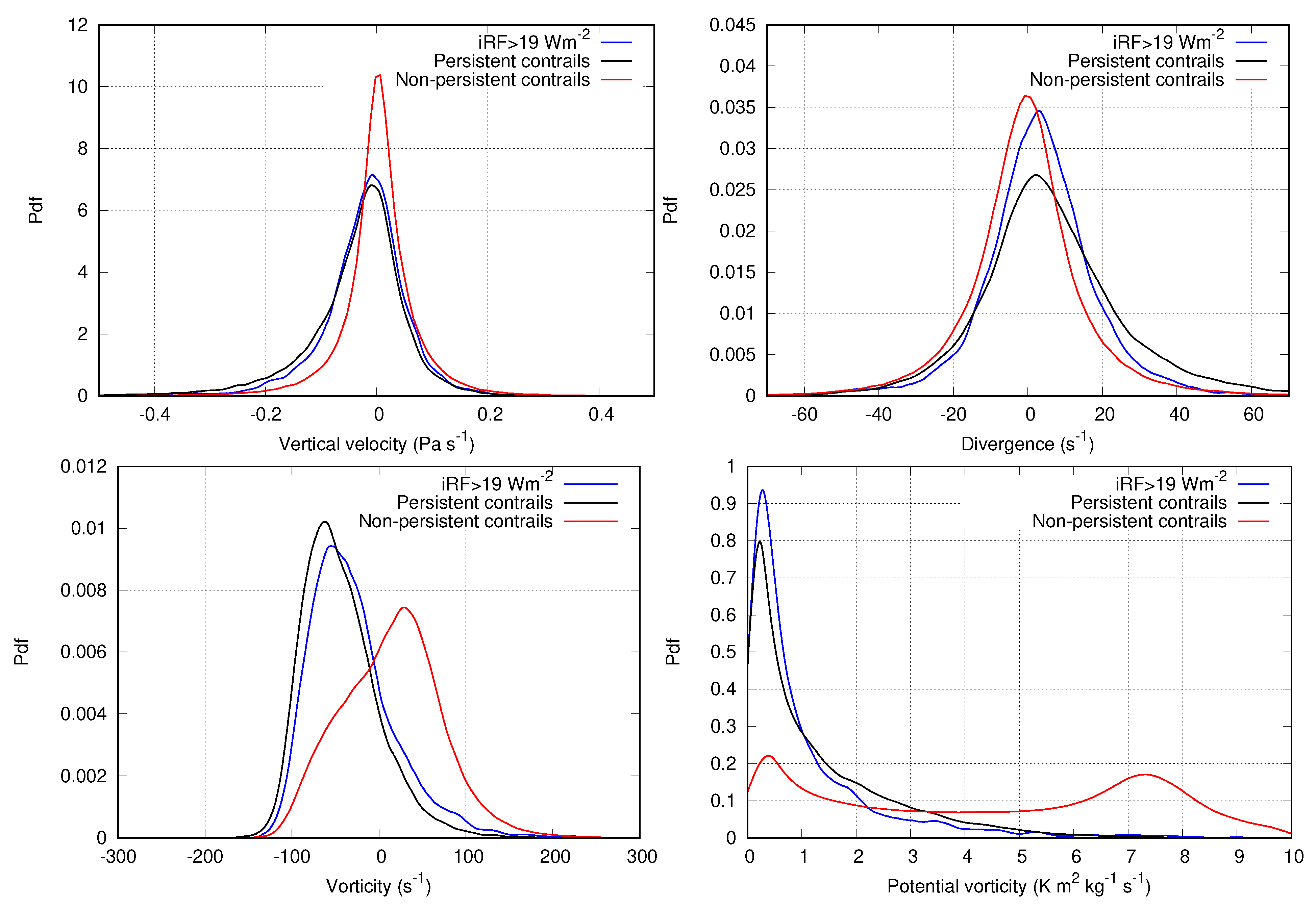
The pdfs for vertical velocity (shown in pressure coordinates, that is, negative values indicate upward motion) are centred around zero (Figure 4, top left). The range was restricted for a better distinction of the curves, excluding values with too low probability densities at the upper and lower end of the distribution. For persistent contrails, the distributions are slightly shifted towards the left, such that the mode values are negative. This favouring of ascending motion can be explained by the formation mechanism of ice-supersaturated regions (ISSRs), which are typically formed when air masses move upwards, where adiabatic cooling leads to an increase of relative humidity.

Similar to the vertical velocity, the pdfs of the divergence (Figure 4, top right) are centred around zero as well, with the blue and back lines for persistent contrails and persistent contrails with large iRF slightly shifted towards positive values. Positive values indicate a divergence, and negative values a convergence, of air masses. As most ISSRs occur in a 200 hPa thick layer below the tropopause [18], this shift is probably caused by the outwards spreading of air masses below the tropopause, which acts as a vertical boundary. The large $R{H}_i$ values in this layer promote the development of persistent contrails with high iRF. This is connected to the potential vorticity (Figure 4, bottom right). The extratropical dynamical tropopause is typically found at the 2 PVU potential vorticity surface [19] (1 PVU $={10}^{-6}$ K m${}^2$ kg${}^{-1}$ s${}^{-1}$), which is why the pdfs for persistent contrails have their peaks below that level. Contrails also develop in the lower stratosphere, but only rarely. The low probability densities at higher PV values of the blue and black function confirm this. Potential vorticity strongly increases in the stratosphere, which explains the difference in the pdf distribution for the general case.

The distributions for the relative vorticity (Figure 4, bottom right) show a large separation between the pdf for the general case (red) and the other two functions. The pdfs for large-iRF (blue) and persistent contrails (black) are narrower and strongly concentrated on the negative side (anticyclonal, clockwise motion) compared to the general case, where the mode value of the distribution is clearly positive (anticlockwise motion). The results agree with [7], since ISSRs also prefer divergent, anticyclonic flow. This variable may help to predict the persistence of contrails, but not to distinguish between persistent contrails of any iRF and those with large iRF, as their density functions still overlap substantially. The overlap in the distributions of the dynamical variables demonstrates that persistent contrails do not only develop during their favoured flow patterns. Only the relative frequency of the patterns is different within and outside of a situation where persistent contrails develop. Therefore, the dynamical fields vertical velocity, divergence, vorticity, and potential vorticity alone are not sufficient to improve the prediction of persistent contrails.

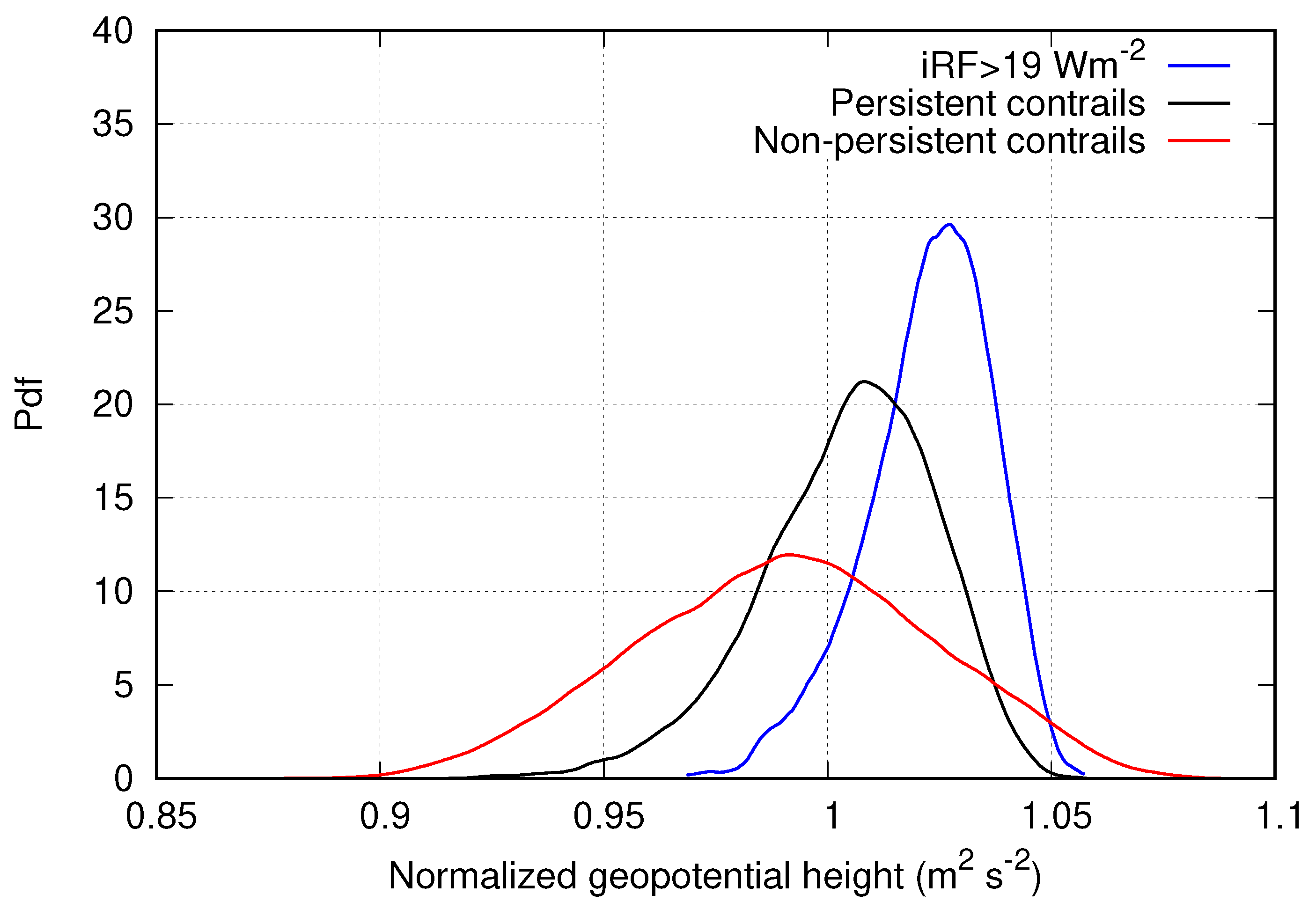
The distributions for the normalised geopotential height (Z) (Figure 5) display the largest separation so far. Persistent contrails are centred around higher Z values (mode values exceeding 1) than cases without persistent contrails (mode value below 1). Persistent contrails with high iRF are more concentrated to the high values of Z than persistent contrails in general; they are specifically found on the top altitudes of the pressure levels.

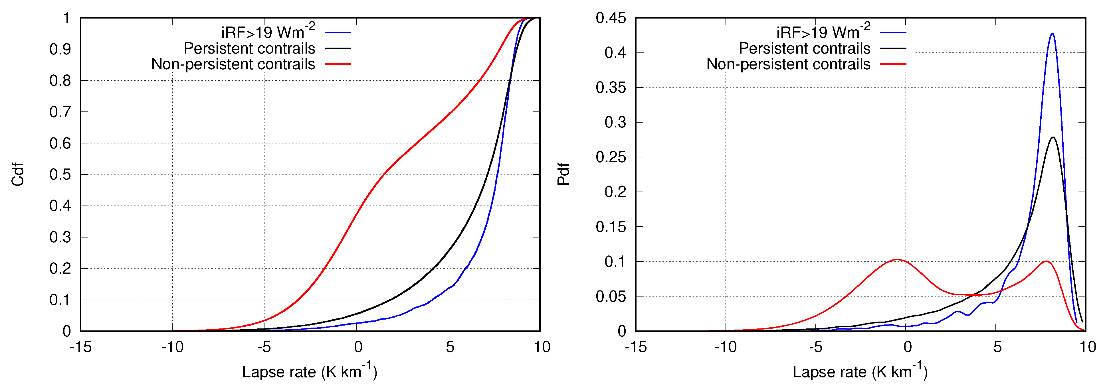
The variable that seems best suited for an improved prediction of the persistence of contrails is the local lapse rate. It describes the vertical temperature gradient and is a measure for the stability of the atmosphere (stratification). The difference between the three scenarios (persistence with large iRF, persistence, and non-persistence) is best visible when looking at the cumulative distribution functions (cdfs) in Figure 6, left. The lapse rates range from about $-15$ to nearly 10 K km${}^{-1}$. While roughly 70% of the cases that don’t allow persistent contrails or no contrails at all have a lapse rate below 5 K km${}^{-1}$, such low values occur only in about 25% of situations that allow persistent contrails and even less (about 15%) so if the latter have a large iRF. However, 20% of persistent contrails occur in air masses with lapse rates exceeding about 8 K km${}^{-1}$, and such high values do hardly occur in situations that do not allow contrail formation or persistence. Hence, persistent contrails and, in particular, persistent contrails with high iRF develop under rather high lapse rates with a weak stratification. Negative lapse rates occur with temperature inversions, which happen when the tropopause is close to the flight level. For physical explanations of the relation between ice supersaturation (i.e., contrail persistence) and high local lapse rates, see [16].

Using the dynamical variables that showed the strongest separation (lapse rate, geopotential height, vorticity, and potential vorticity) and combining them with the Schmidt-Appleman quantities temperature and relative humidity could enable an improved prediction for contrail persistence based on atmospheric conditions along a flight. For the lapse rate and the geopotential height, the pdf of persistent contrails with large iRF is separated from the pdf of general persistent contrails. This could additionally allow a prediction of particularly strong warming contrails. Specifically avoiding those could reduce the overall radiative effect of contrail cirrus significantly [8].

3.3. Path-Length Statistics for High Instantaneous Radiative Forcings and Big Hits

“Big Hits” are contrails with a very high individual energy forcing (EF), which is the integral of iRF over a contrail’s area and lifetime. Of course, these contrails are primary candidates for avoidance. Although we cannot determine EF-integrals from the single iRF values in our data set, we can get closer to EF by considering consecutive iRF values as they occur along a flight; that is, instead of probing a small sample of records as before, we now take all measured values into account. We use all data in order to find consecutive points along the flight tracks with an iRF value above the 19 W m${}^{-2}$ threshold mentioned before (i.e., the iRF long term mean plus one standard deviation). A long track with high iRF values more likely forms a Big Hit than single scattered high-iRF records and avoidance of Big Hits by flight diversion is only feasible if they have a certain spatial extension.

To analyze this, a second dataset was produced from the ten years of MOZAIC’s flights with all data. Consecutive records with an iRF in excess of 19 W m${}^{-2}$ are stored each in its own data file. If the threshold is undercut for a short distance of less than 10 data records (corresponding to 40 s of flight or about ten kilometres), we consider this a small fluctuation that does not interrupt a Big Hit; only if the gap is larger, we close the current file and proceed to the next record with an iRF in excess of the threshold. In this way, we find 13,955 Big Hits.

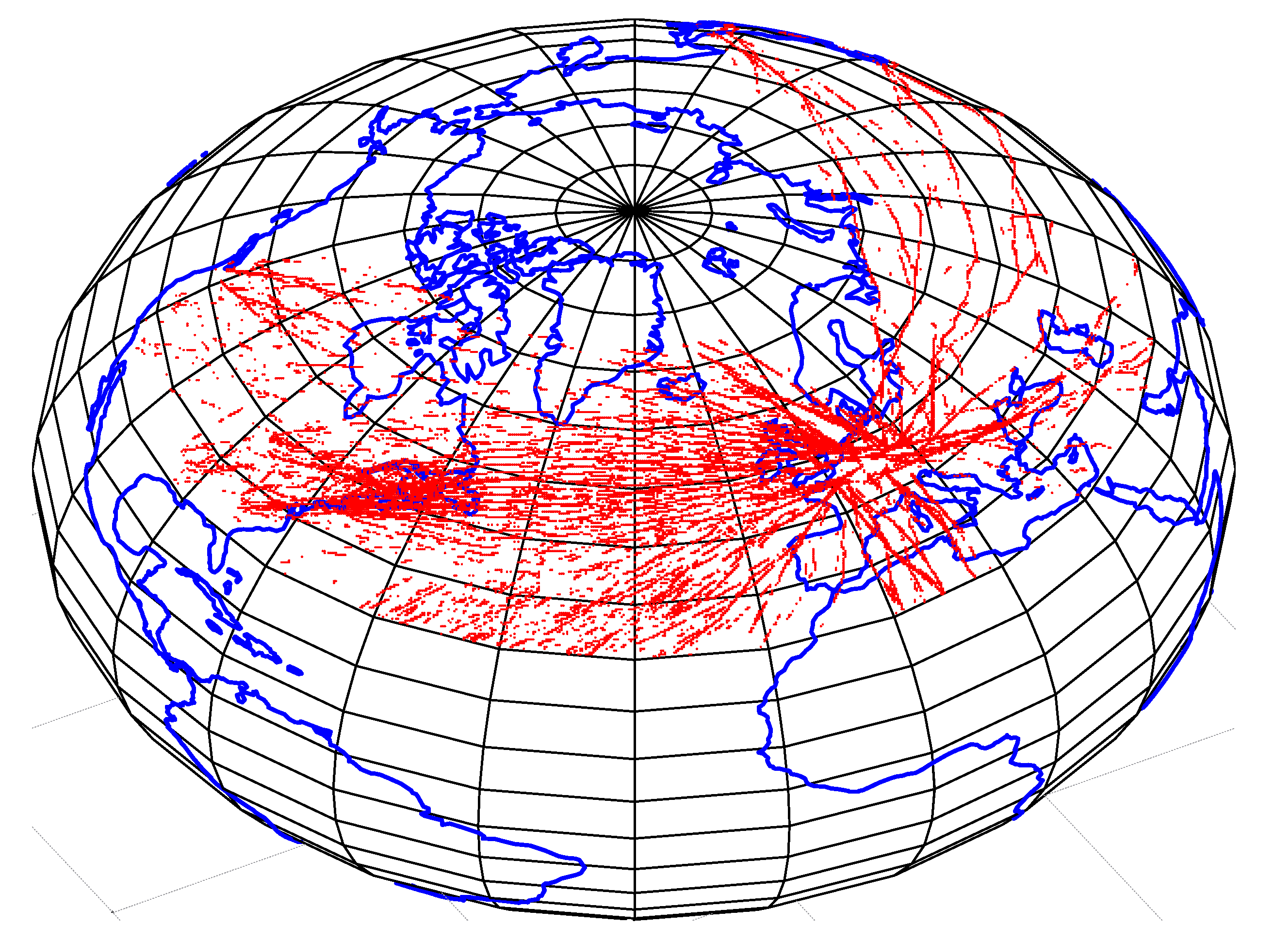
First, we check whether the so-defined Big Hits occur everywhere or perhaps only in special regions. For this, their coordinates are plotted on a world map (see Figure 7) centred on the North-Atlantic flight corridor. This map gives only a weak indication of regions where Big Hits do not occur, where they are perhaps less probable over Greenland. Otherwise, the distribution of the red dots resembles the general distribution of MOZAIC flights within the considered mid-latitude belt. The distribution of red dots is more homogeneous in the main traffic regions than in less-frequented ones, probably because there are simply more data. In regions with fewer flights, the Big Hit locations seem to be a bit scattered or patchy along the track. This is likely caused by the strong variations in the atmospheric relative humidity field. When Big Hits do not always form as coherent tracks along the flight path, the question arises, whether, when, and where their avoidance by flight diversion makes sense. Preventing Big Hits is only effective if they do not appear pointwise and have more than a few kilometres in length. This length should be a not too small fraction of the mean path length of aircraft within ISSRs, that is, 150 km [20].

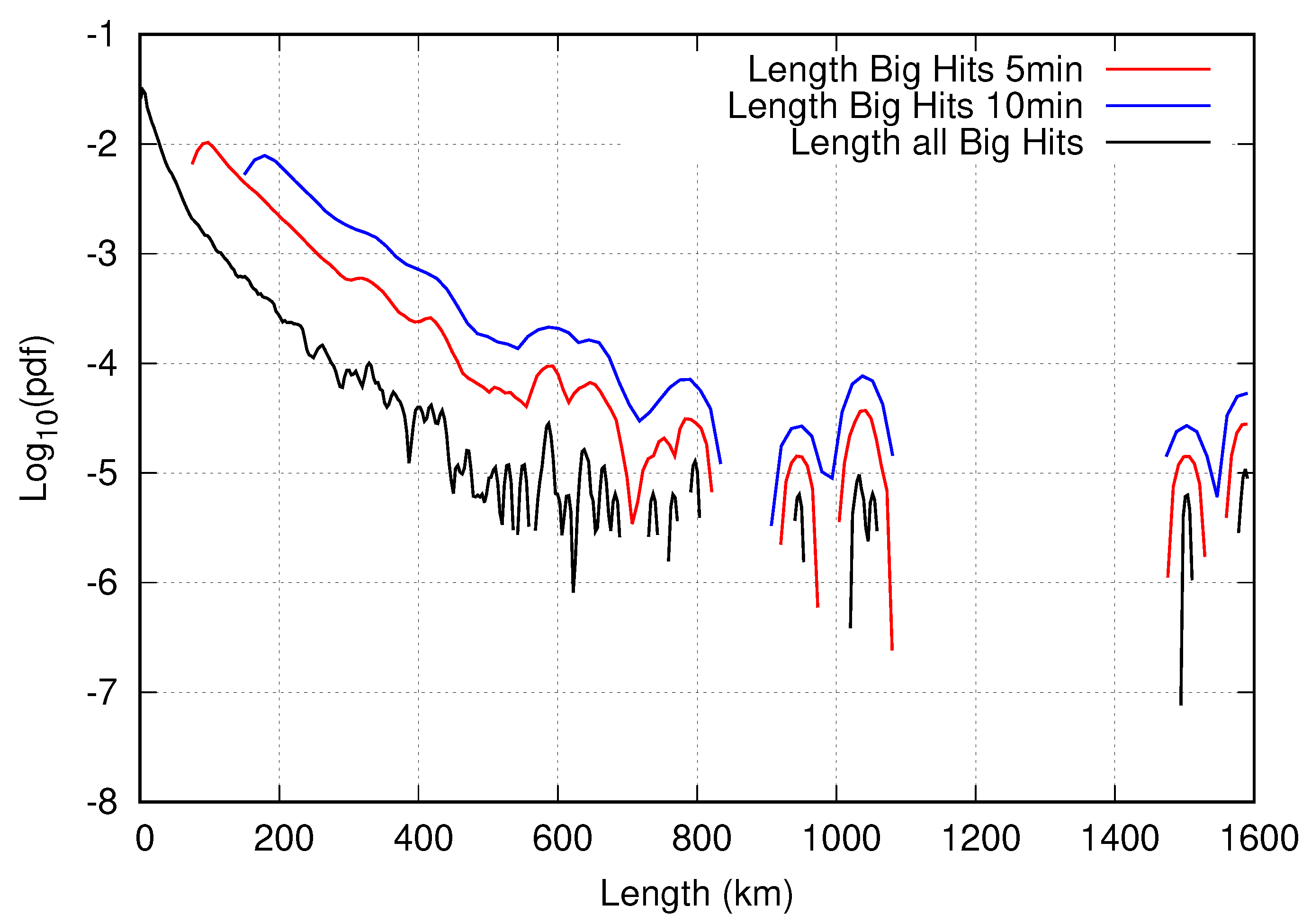
To examine this, the path lengths of each of the 13,955 Big Hits were calculated, see Figure 8. The majority (12,131) have a length less than 75 km (which translates to a flight duration of 5 minutes). Only 13% (1864) of Big Hits have an extension above 75 km and only 5% (660) have path lengths above 150 km. (Of course, these fractions depend on the chosen threshold iRF $\ge 19$ W m${}^{-2}$ and the assumptions mentioned above). The path length distributions of Big Hits exceeding 75 km (red) and 150 km (blue) follow roughly an exponential decline for the first 600 to 800 km. The dataset contains one Big Hit exceeding 1500 km in length. Although those occur very rarely, their climate effect is above average (WGR21). Preventing the development of such contrails could make a huge difference. Ref. [21] is a good example for that. In their data, about 2% of the flights in the Japanese airspace contributed to 80% of the energy forcing in the region (over a study period of six weeks in total).

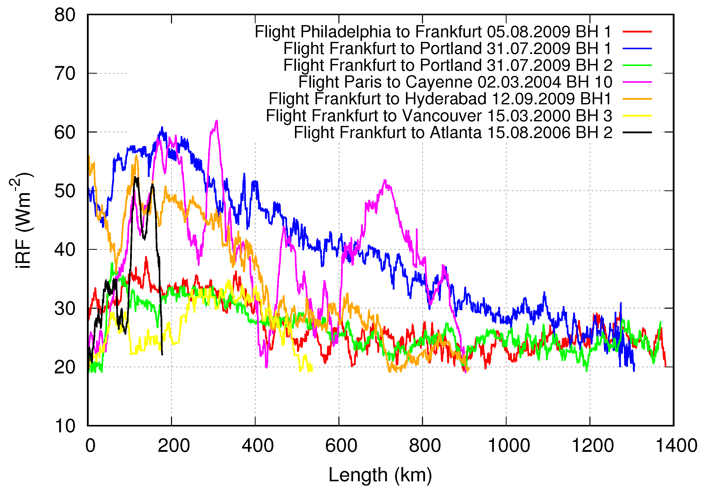
However, it is also important to look at the coherence of the iRF itself. If the iRF changes strongly in a matter of seconds, it would not be possible to adjust the flight level accordingly. Figure 9 shows the iRF along randomly chosen flights of different lengths. The coloured curves illustrate that the iRF jumps only weakly up and down from one flight point to another (4 s or 1 km apart) with an amplitude of approximately 5 W m${}^{-2}$ (blue, red, and green curves). Some of the curves (pink and orange) reveal strong fluctuations. This could be caused by a change in the surroundings along the flight path, e.g., by the presence of a natural cirrus or another contrail, or changing surface characteristics, e.g., when flying above a coast vs. above a dark ocean. Passing the terminator line, which separates day and night on the globe, could also induce such variations of iRF. In total, the results are encouraging, as the iRF does not constantly vary from a very high to a low value from one flight point to the next. Furthermore, for actual avoidance, one would consider integral values (e.g., EF) which are smoother than the underlying iRF time series. This is beneficial for flight diversion strategies.

3.4. Discussion

The iRF values necessary to distinguish Big Hits from weaker contrails are computed from the temperature and humidity measured by MOZAIC aircraft in cruise and ERA-5 radiation quantities interpolated to the aircraft positions (see WGR21). Thus, they refer to contrails at the very moment of their formation. It is, however, not obvious that a large iRF of this kind implies a strongly warming contrail, that is, a contrail with a large energy forcing [22]. If there is a correlation between iRF and EF, it is probably, at most, a weak one. A test calculation using a small data set by U. Schumann (private communication, 2021) did not yield a correlation, while a weak correlation between the initial contrail volume and ice mass to the integrated shortwave impact is indicated in [23]. In any case, a large EF needs more than just a high iRF at the moment of contrail formation. EF includes the area a contrail spans in the sky and, in particular, the contrail life-time as well as the distribution of optical thickness over this area (both together can be combined into the so called total extinction, see [24]). These factors cannot be captured by a single data record. Contrail lateral growth depends on the local vertical wind shear component perpendicular to the flight direction. While this quantity could be obtained from forecast or reanalysis data, it still does not suffice to determine the effective width for the EF calculation since the optical properties (from ice mass and ice number concentration) and the radiation background (e.g., other clouds and contrails, surface albedo) change during the expansion of the contrail in ways that are virtually unpredictable for a weather forecast model. The lifetime of a contrail depends on synoptic conditions and the growth rate and sedimentation of the ice crystals [25].

Thus, the only connection of high local iRF values and actually strongly warming contrails, those with high EF values, can be seen in our cases with many consecutive high iRF values. It is probable that a >75 km track of high iRF values will coincide with a contrail of higher-than-average EF. Probably such a track crosses a larger area that allows a cluster of strong contrails if air traffic density there is sufficient e.g., [26]. If Big Hits, in the EF sense, would predominantly occur in clusters, it should be easier to predict them as if they would occur in isolation. It is not required to know the air traffic in advance; likely it suffices to mark regions on the weather charts as regions of potential Big Hits, and the demarcation of such regions would involve the conditional distributions determined in this paper combined with the radiation parameterisation of [15]. Only the estimation of contrail optical thicknesses (which needs the actual supersaturation value) is not straightforward since, for the prediction purpose, one is restricted to the forecasted humidity field. Thus, it is not sufficient to predict ice supersaturation per se but also to estimate a mean or maximum degree of ice supersaturation in a predicted ISSR. This is still an open issue for future work.

4. Summary and Conclusions

This paper is concerned with improving the capabilities of predicting persistent contrails for the purpose of contrail avoiding flight routing, a necessary step on the way to green flight aspirations. Recognising the principal difficulties to forecast relative humidity in general and ice supersaturation in particular, it resorts to proxy variables that may have characteristic signatures in situations that allow persistent contrails or even strong endothermic persistent contrails. Therefore, it presents conditional probability distributions for a variety of thermodynamic and dynamic quantities characterizing the upper troposphere at northern midlatitudes: temperature, water vapour concentration and relative humidity, vertical wind speed and divergence, relative and potential vorticity, normalised geopotential, and lapse rate. The three conditions under which these distributions are determined are: (a) contrail formation impossible or contrails not persistent; (b) contrails possible and persistent; and (c) contrails possible, persistent, and strongly endothermic. These conditions are determined from airborne data from the MOZAIC measurement program, while the atmospheric quantities are taken from ERA-5 reanalyses, interpolated to the position of the respective MOZAIC aircraft. The conditional distributions are determined from 10 years of data, 2000–2009.

It turns out that some quantities have strongly overlapping distributions for contrail and non-contrail situations. Vertical wind speed and divergence are not appropriate proxy variables. Relative vorticity and potential vorticity are more apt, since their conditional distributions are distinct. For instance, contrails prefer anticyclonic airmasses while the pdf for situations without persistent contrails peaks in cyclonic rotation. Persistent contrails are very rare in the stratosphere; therefore, a potential vorticity exceeding 2 to 3 PVU has a low probability under such a condition, while there is no such constraint in the general case without contrails.

Perhaps a bit surprisingly, the variables with the strongest signatures for persistent contrails are the normalised geopotential height and the lapse rate. Even the two contrail classes (any iRF value and large iRF value) show distinct probability distributions. Thus, we hope that these fields can not only be exploited as very good proxies for improved contrail prediction, but perhaps even as indicators of the warming potential of the predicted contrails. Combining these proxies into a probabilistic prediction method for contrail persistence is ongoing work.

In a further investigation, we showed that often high values of iRF occur in isolation, but sometimes there are quite long tracks where each value of iRF exceeds the selected threshold (19 W m${}^{-2}$). We deem that such situations point to true Big Hits, namely contrails that not only display a large iRF value at the time of their formation, but over a large fraction of their length and lifetime. Perhaps such regions also have a large horizontal extension such that clusters of strong contrails would form in the case of heavy air traffic in this region. It is surely easier to predict extended supersaturated areas than small patches with high RHi. Thus, the quest for a reliable prediction method for Big Hits seems to have a real chance, which will profit from the exploitation of dynamical proxies. Making this method work is on our research agenda for the near future.

References

1. Lee, D.; Fahey, D.; Skowron, A.; Allen, M.; Burkhardt, U.; Chen, Q.; Doherty, S.; Freeman, S.; Forster, P.; Fuglestvedt, J.; et al. The contribution of global aviation to anthropogenic climate forcing for 2000 to 2018. Atmos. Environ. 2021, 244, 117834. [Google Scholar] [CrossRef] [PubMed]
2. Schumann, U. On conditions for contrail formation from aircraft exhausts. Meteorol. Z. 1996, 5, 4–23. [Google Scholar] [CrossRef]
3. Gierens, K.; Spichtinger, P.; Schumann, U. Ice supersaturation. In Atmospheric Physics. Background—Methods—Trends; Schumann, U., Ed.; Springer: Berlin/Heidelberg, Germany, 2012; Chapter 9; pp. 135–150. [Google Scholar]
4. Gierens, K.; Matthes, S.; Rohs, S. How well can persistent contrails be predicted? Aerospace 2020, 7, 169. [Google Scholar] [CrossRef]
5. Mazon, J.; Pino, D. A WRF simulation of an episode of contrails covering the entire sky. Atmosphere 2016, 7, 95. [Google Scholar] [CrossRef] [Green Version]
6. Immler, F.; Treffeisen, R.; Engelbart, D.; Krüger, K.; Schrems, O. Cirrus, contrails, and ice supersaturated regions in high pressure systems at northern mid latitudes. Atmos. Chem. Phys. 2008, 8, 1689–1699. [Google Scholar] [CrossRef] [Green Version]
7. Gierens, K.; Brinkop, S. Dynamical characteristics of ice supersaturated regions. Atmos. Chem. Phys. 2012, 12, 11933–11942. [Google Scholar] [CrossRef] [Green Version]
8. Wilhelm, L.; Gierens, K.; Rohs, S. Weather variability induced uncertainty of contrail radiative forcing. Aerospace 2021, 8, 332. [Google Scholar] [CrossRef]
9. Marenco, A.; Thouret, V.; Nedelec, P.; Smit, H.; Helten, M.; Kley, D.; Karcher, F.; Simon, P.; Law, K.; Pyle, J.; et al. Measurement of ozone and water vapor by Airbus in-service aircraft: The MOZAIC airborne program, An overview. J. Geophys. Res. 1998, 103, 25631–25642. [Google Scholar] [CrossRef]
10. Petzold, A.; Thouret, V.; Gerbig, C.; Zahn, A.; Brenninkmeijer, C.; Gallagher, M.; Hermann, M.; Pontaud, M.; Ziereis, H.; Boulanger, D.; et al. Global-scale atmosphere monitoring by in-service aircraft - current achievements and future prospects of the European Research Infrastructure IAGOS. Tellus B 2015, 67, 28452. [Google Scholar] [CrossRef] [Green Version]
11. Hersbach, H.; Bell, B.; Berrisford, P.; Biavati, G.; Horányi, A.; Muñoz Sabater, J.; Nicolas, J.; Peubey, C.; Radu, R.; Rozum, I.; et al. ERA5 hourly data on single levels from 1979 to present. In Copernicus Climate Change Service (C3S) Climate Data Store (CDS); Technical Report; ECMWF: Reading, UK, 2018. [Google Scholar] [CrossRef]
12. Hersbach, H.; Bell, B.; Berrisford, P.; Biavati, G.; Horányi, A.; Muñoz Sabater, J.; Nicolas, J.; Peubey, C.; Radu, R.; Rozum, I.; et al. ERA5 hourly data on pressure levels from 1979 to present. In Copernicus Climate Change Service (C3S) Climate Data Store (CDS); Technical Report; ECMWF: Reading, UK, 2018. [Google Scholar] [CrossRef]
13. Hersbach, H.; Bell, B.; Berrisford, P.; Hirahara, S.; Horányi, A.; Muñoz Sabater, J.; Nicolas, J.; Peubey, C.; Radu, R.; Schepers, D.; et al. The ERA5 global reanalysis. Quart. J. Roy. Met. Soc. 2020, 146, 1999–2049. [Google Scholar] [CrossRef]
14. Copernicus Climate Change Service (C3S). ERA5: Fifth generation of ECMWF atmospheric reanalyses of the global climate. Copernic. Clim. Chang. Serv. Clim. Data Store (CDS) 2017, 15, 2020. [Google Scholar]
15. Schumann, U.; Mayer, B.; Graf, K.; Mannstein, H. A parametric radiative forcing model for contrail cirrus. J. Appl. Meteorol. Climatol. 2012, 51, 1391–1406. [Google Scholar] [CrossRef] [Green Version]
16. Gierens, K.; Wilhelm, L.; Hofer, S.; Rohs, S. The effect of ice supersaturation and thin cirrus on lapse rates in the upper troposphere. Atmos. Chem. Phys. Discuss. 2022, 22, 1–18. [Google Scholar] [CrossRef]
17. Silverman, B.W. Density Estimation for Statistics and Data Analysis; Number 26 in Monographs on Statistics and Applied Probability; Chapman and Hall/CRC: Boca Raton, FL, USA, 1998. [Google Scholar]
18. Spichtinger, P.; Gierens, K.; Leiterer, U.; Dier, H. Ice supersaturation in the tropopause region over Lindenberg, Germany. Meteorol. Z. 2003, 12, 143–156. [Google Scholar] [CrossRef]
19. Holton, J.; Haynes, P.; McIntyre, M.; Douglass, A.; Rood, R.; Pfister, L. Stratosphere-troposphere exchange. Rev. Geophys. 1995, 33, 403. [Google Scholar] [CrossRef]
20. Gierens, K.; Spichtinger, P. On the size distribution of ice–supersaturated regions in the upper troposphere and lowermost stratosphere. Ann. Geophys. 2000, 18, 499–504. [Google Scholar] [CrossRef]
21. Teoh, R.; Schumann, U.; Majumdar, A.; Stettler, M. Mitigating the climate forcing of aircraft contrails by small-scale diversions and technology adoption. Environ. Sci. Technol. 2020, 54, 2941–2950. [Google Scholar] [CrossRef]
22. Schumann, U.; Graf, K.; Mannstein, H. Potential to reduce climate impact of aviation by flight level changes. In Proceedings of the 3rd AIAA Atmospheric Space Environments Conference, Honolulu, HI, USA, 27–30 June 2011; p. 3376. [Google Scholar] [CrossRef] [Green Version]
23. Burkhardt, U.; Bock, L.; Bier, A. Mitigating the contrail cirrus climate impact by reducing aircraft soot number emissions. NPJ Clim. Atmos. Sci. 2018, 37, 1–7. [Google Scholar] [CrossRef] [Green Version]
24. Unterstrasser, S.; Gierens, K. Numerical simulations of contrail-to-cirrus transition—Part 1: An extensive parametric study. Atmos. Chem. Phys. 2010, 10, 2017–2036. [Google Scholar] [CrossRef] [Green Version]
25. Bier, A.; Burkhardt, U.; Bock, L. Synoptic control of contrail cirrus lifecycles and their modification due to reduced soot number emissions. J. Geophys. Res. 2017, 122, 11584–11603. [Google Scholar] [CrossRef] [Green Version]
26. Bock, L.; Burkhardt, U. Reassessing properties and radiative forcing of contrail cirrus using a climate model. J. Geophys. Res. 2016, 121, 97179736. [Google Scholar] [CrossRef] [Green Version]
Figure 1. Temperature probability density functions (pdfs) in general situations without persistent contrails (red), in situations that allow persistent contrails (black), and in situations for persistent contrails that have a particularly large iRF (blue). The pdfs comprise the temperatures that ERA-5 reanalysis data show for the respective flight points from MOZAIC. Note that the deciding factors for persistence are MOZAIC’s thermodynamic quantities.
Applsci 12 04450 g001
Figure 2. As Figure 1, but for absolute humidity in terms of water vapour mass concentration (in logarithmic scale).
Applsci 12 04450 g002
Figure 3. As Figure 1, but for R H max (left panel) and R H i (right panel).
Applsci 12 04450 g003
Figure 4. As Figure 1, but for vertical velocity (in pressure coordinates, upper left panel), divergence (upper right), relative vorticity (lower left panel), and potential vorticity (lower right panel).
Applsci 12 04450 g004
Figure 5. As Figure 1, but for normalised geopotential height.
Applsci 12 04450 g005
Figure 6. Left panel: cumulative distribution functions (cdfs) of lapse rates found in situations without persistent contrails (red), with persistent contrails (black), and with persistent contrails with large iRF (blue). Right panel: The probability density functions corresponding to the cdfs in the right panel.
Applsci 12 04450 g006
Figure 7. Map of the world centred on the north-Atlantic flight corridor. Every red dot marks a location where the combination of MOZAIC and ERA-5 data indicated a quite large instantaneous radiative forcing value for a persistent contrail at its formation, iRF > 19 W m 2 . Note that only flights in the northern midlatitude band 30 ° to 70 ° are analysed. The figure indicates that a large iRF can occur almost everywhere.
Applsci 12 04450 g007
Figure 8. Path length distribution (pdf) for flight tracks with consecutive iRF 19 W m 2 . The black curve shows the unconditioned distribution, which includes a lot of such strong events that are too short for rerouting an aircraft. The red and blue curves show the pdfs conditioned on a minimum path length or duration that an aircraft is flying under such conditions. Note the strong noise at large path lengths; the events that contribute there are essentially single cases.
Applsci 12 04450 g008
Figure 9. Time series of iRF values in a number of situations with consecutive iRF 19 W m 2 that occurred on the flights indicated in the figure.
Applsci 12 04450 g009
Publisher’s Note: MDPI stays neutral with regard to jurisdictional claims in published maps and institutional affiliations.