Outlier Reconstruction of NDVI for Vegetation-Cover Dynamic Analyses

Abstract

The normalized difference vegetation index (NDVI) contains important data for providing vegetation-cover information and supporting environmental analyses. However, understanding long-term vegetation cover dynamics remains challenging due to data outliers that are found in cloudy regions. In this article, we propose a sliding-window-based tensor stream analysis algorithm (SWTSA) for reconstructing outliers in NDVI from multitemporal optical remote-sensing images. First, we constructed a tensor stream of NDVI that was calculated from clear-sky optical remote-sensing images corresponding to seasons on the basis of the acquired date. Second, we conducted tensor decomposition and reconstruction by SWTSA. Landsat series remote-sensing images were used in experiments to demonstrate the applicability of the SWTSA. Experiments were carried out successfully on the basis of data from the estuary area of Salween River in Southeast Asia. Compared with random forest regression (RFR), SWTSA has higher accuracy and better reconstruction capabilities. Results show that SWTSA is reliable and suitable for reconstructing outliers of NDVI from multitemporal optical remote-sensing images.

1. Introduction

Global climate change has led to sea-level rise, desertification, and biodiversity losses [1,2]. Vegetation cover is a sensitive indicator of climate change that feeds back to it by influencing energy, water, and carbon cycles [1,3,4]. Variability in vegetation cover represents one of the main sources of systematic changes over Earth’s surface at different spatial scales [5,6]. Such changes are especially evident in areas of concentrated terrestrial, oceanic, and atmospheric interactions, such as in estuarine coastal zones. The identification of patterns in vegetation-cover dynamics is paramount for a greater understanding of ecological responses of natural ecosystems to global climate change [3,7]. The normalized difference vegetation index (NDVI), a near real-time vegetation index that is derived from optical remote-sensing images is often used as a proxy for vegetation-cover variance. Fine NDVI relies on clear-sky pixels in high-resolution optical remote-sensing images [8,9].

Remote-sensing techniques with temporal continuity and large spatial coverage provide effective and comprehensive means for the accurate estimation of vegetation-cover conditions [3,9]. The number of remote sensors capable of acquiring appropriate temporal data has increased considerably within the last few years [9,10,11]. With routine time-series observations, satellite remote sensing provides an unprecedented capability for estimating vegetation cover and its spatiotemporal variability at different spatial scales [3,11,12]. However, clouds cover roughly half of Earth [13,14]. Persistent cloud cover poses significant challenges for the acquisition of clear terrestrial optical remotely sensed imagery [14,15,16]. This occlusion produces a large number of outliers that are a persistent barrier to the operational monitoring of vegetation for many regions of the world, especially in Southeast Asia during the summer months [14,17,18]. Reconstructing the values of cloud-covered pixels in optical remote-sensing imagery is crucial because outliers in images can produce misleading results in environmental analyses [19,20,21].

Numerous algorithms were developed to reconstruct NDVI outliers for vegetation estimation over the past few years. Spatial-information-based methods are typically proposed on the basis of the spatial correlation between target pixels and neighboring clear-sky pixels [22,23]. Other approaches are multisatellite data-fusion algorithms that combine information from multiple sensors with different spatial, spectral, and temporal resolutions to generate merged products with high spatiotemporal resolution [16,24,25]. Lastly, state-of-the-art machine-learning algorithms are used to reconstruct NDVI [26,27]. Tensor stream analysis is a fundamental model in machine learning, especially in the field of computer vision and image processing [21,28]. In recent years, tensor decomposition was verified to be effective in capturing global low-rank correlation for tensor recovery tasks. A fast low-rank tensor completion method was proposed for reducing dimensions of color images, MRI, and videos [29]. The tensor decomposition model is being paid much attention in outlier reconstruction for remote-sensing images. Low-rank tensor completion methods based on tensor singular-value decomposition and core tensor minimization were proposed [30]. However, accurately reconstructing NDVI for cloud-covered pixels is an urgent issue in widening NDVI-based applications [31,32,33].

To improve the accuracy of vegetation cover analyses, we explored a novel reconstruction algorithm for outliers on the basis of the Tucker decomposition method and sliding-window-based tensor stream analysis. Landsat series remote-sensing images are used in experiments to demonstrate the applicability of the proposed approach. As a case study, we successfully reconstructed NDVI in an estuary of Salween River in Southeast Asia. The proposed method is reliable and suitable for reconstructing outliers in cloud-covered pixels. This is one of only a few studies that used tensor stream analysis to reconstructive NDVI in the Salween River Basin.

2. Materials and Methods

2.1. Datasets

Experimental analysis was performed on datasets for the estuary of Salween River (Figure 1a). Salween River is one of only a few long free-flowing rivers in Southeast Asia, originating in the Tibet Plateau and emptying into the Andaman Sea in the Indian Ocean [34]. On the basis of Shuttle Radar Topography Mission (SRTM) data, Figure 1a,b show the location and digital elevation model (DEM) of the study area, an area of about $3.6\times {10}^3{\mathrm{km}}^2$. We used optical remote-sensing images acquired by Landsat series satellite from the summer of 1973 to the summer of 2020. Unfortunately, the majority of summer images included a large number of outliers in cloud-covered pixels. Clear-sky images that could be used for deriving NDVI are from winter.

Table 1. Optical remote-sensing images of study area from 1973 to 2020.

Datasets	Acquired Date	Platform	Spatial Resolution
Training	4 March 1973	Landsat 1	60 m × 60 m
	22 January 1974	Landsat 1	60 m × 60 m
	27 December 1978	Landsat 3	60 m × 60 m
	19 February 1979	Landsat 3	60 m × 60 m
	25 February 1988	Landsat 5	30 m × 30 m
	19 January 1989	Landsat 4	30 m × 30 m
	18 March 1990	Landsat 5	30 m × 30 m
	16 January 1991	Landsat 5	30 m × 30 m
	4 February 1992	Landsat 5	30 m × 30 m
	6 February 1993	Landsat 5	30 m × 30 m
	14 April 1994	Landsat 5	30 m × 30 m
	12 February 1995	Landsat 5	30 m × 30 m
	30 January 1996	Landsat 5	30 m × 30 m
	1 February 1997	Landsat 5	30 m × 30 m
	4 February 1998	Landsat 5	30 m × 30 m
	7 February 1999	Landsat 5	30 m × 30 m
	10 February 2000	Landsat 5	30 m × 30 m
	12 February 2001	Landsat 5	30 m × 30 m
	23 February 2002	Landsat 7	30 m × 30 m
	25 January 2003	Landsat 7	30 m × 30 m
	8 March 2004	Landsat 5	30 m × 30 m
	7 February 2005	Landsat 5	30 m × 30 m
	14 March 2006	Landsat 5	30 m × 30 m
	2 April 2007	Landsat 5	30 m × 30 m
	16 December 2008	Landsat 5	30 m × 30 m
	2 February 2009	Landsat 5	30 m × 30 m
	21 February 2010	Landsat 5	30 m × 30 m
	8 February 2011	Landsat 5	30 m × 30 m
	14 December 2013	Landsat 8	30 m × 30 m
	4 March 2014	Landsat 8	30 m × 30 m
	20 December 2015	Landsat 8	30 m × 30 m
	6 February 2016	Landsat 8	30 m × 30 m
	9 December 2017	Landsat 8	30 m × 30 m
	16 November 2018	Landsat 8	30 m × 30 m
Testing	2 March 2019	Landsat 8	30 m × 30 m
	5 April 2020	Landsat 8	30 m × 30 m

shows the temporal and spatial extent of the experimental dataset. Data were divided into training and testing sets; the former was used to determine the values of algorithm parameters, while the latter was used to evaluate the performance of the proposed algorithm. In this article, we reconstruct outliers of summer NDVI on the basis of the above datasets.

The atmosphere correction method [35,36] was used for remote-sensing images downloaded from the USGS Earth explorer system (https://earthexplorer.usgs.gov, accessed on 19 September 2020). The spatial resolution of all optical remote-sensing images was resampled at 30 × 30 m, and the study area was divided into $2160\times 1866$ pixels (4,030,560 pixels). NDVI image series (Figure 1) were computed on ENVI 5.3 software. We stored all NDVI data in multidimensional arrays to construct the tensor.

2.2. Methods

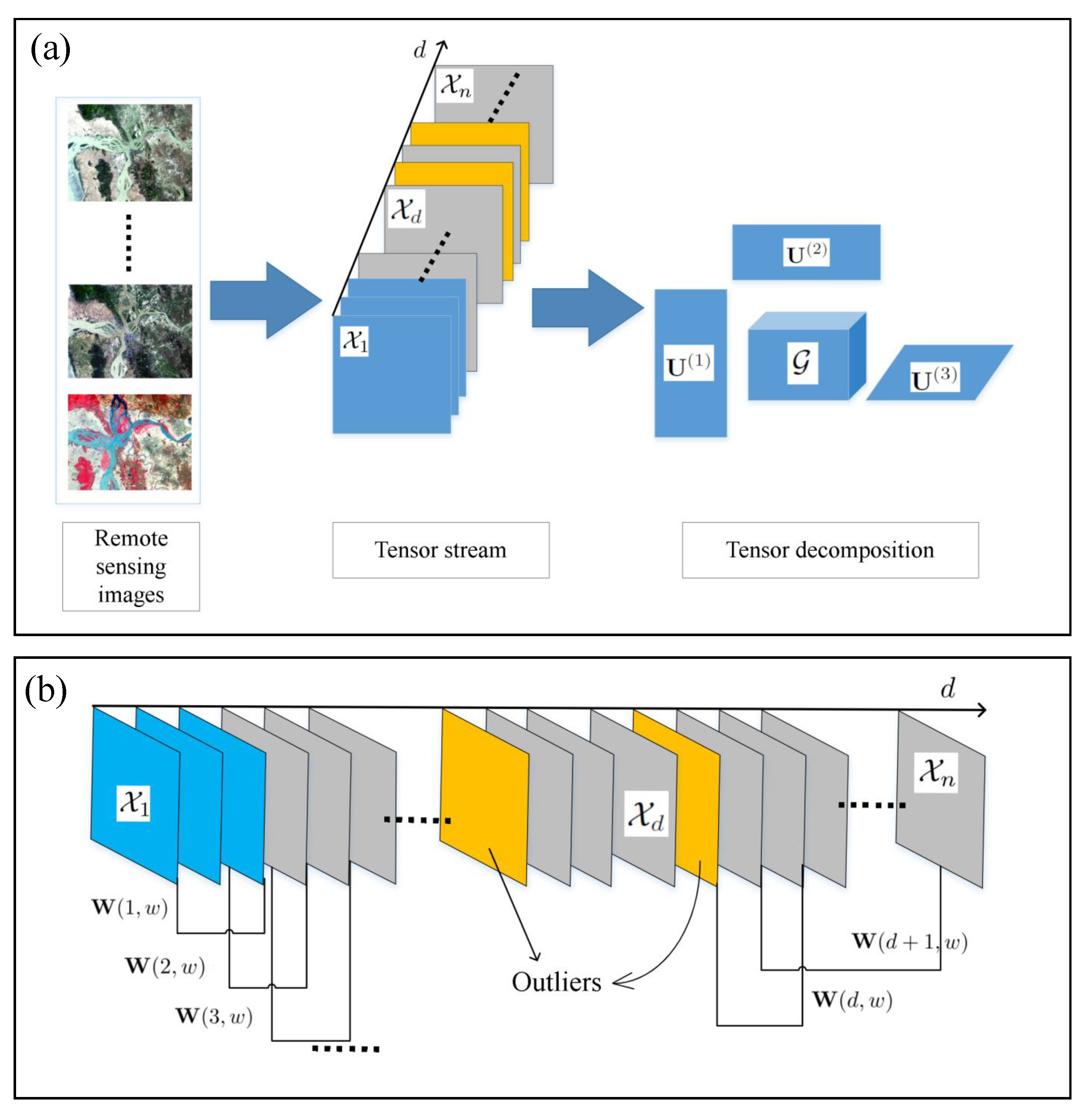
2.2.1. Data Representation

Optical remote-sensing images contain spatial and temporal information about the surface of Earth [37], and are composed of pixels marked with row and column numbers. NDVI is a widely used vegetation index to monitor and project conditions of vegetation cover [38] that can be calculated from optical remote-sensing images as follows [39]

$$\mathrm{NDVI}=\frac{{\rho }_{\mathrm{Nir}}-{\rho }_{\mathrm{Red}}}{{\rho }_{\mathrm{Nir}}+{\rho }_{\mathrm{Red}}},$$

(1)

where ${\rho }_{\mathrm{Nir}}$ and ${\rho }_{\mathrm{Red}}$ represent the near-infrared and red bands of optical remote-sensing images, respectively.

The value of NDVI is between $-1$ and 1; a negative value indicates that the ground is covered with water, snow, etc.; 0 indicates that the ground has rocks or bare ground etc.; and a positive value indicates ground with vegetation. The higher the value is, the greater the vegetation cover. The NDVI of a vegetated area tends toward positive values, whereas water and urban areas are represented by near-zero or negative values [3]. Thus, optical remote-sensing images can be represented as a multidimensional array with NDVI.

2.2.2. Tensor Construction

A tensor is a multidimensional array, and the number of dimensions is called the order of the tensor, also named as ways and modes [40]. In tensor terminology, the order of a tensor $\mathcal{X}\in {\mathbb{R}}^{I_1\times I_2\times \dots \times I_N}$ is N, and the elements of $\mathcal{X}$ are denoted as $a_{i_1{i}_2\dots i_N}$. To model vegetation-cover conditions in different years and the same geographical area under the same spatial resolution, a tensor $\mathcal{X}\in {\mathbb{R}}^{I\times J\times K}$ can be constructed on the basis of NDVI pixels, with the three dimensions standing for row number, column number, and acquired date of pixel, respectively, as shown in Figure 2a. An entry $\mathcal{X}(i,j,k)=c$ denotes that the value of pixel in the i-th row, j-th column and in the k-th year is c.

In tensor terminology, an n-order tensor can be formulated as a matrix by unfolding, and the elements of the tensor are mapped to the matrix.

$$unfol{d}_n\left(\mathcal{X}\right):={\mathbf{X}}_{\left(n\right)}\in {\mathbb{R}}^{I_n\times (I_1\dots I_N)},$$

(2)

and the elements of the tensor are mapped to matrix the element$(i_n,j)$, where

$$j=1+\sum _{\genfrac{}{}{0pt}{}{k=1}{k\ne n}}^N(i_k-1)J_k,\mathrm{with}{J}_k=\prod _{\genfrac{}{}{0pt}{}{N=1}{N\ne n}}^{k-1}{I}_N,$$

(3)

The n-mode product of a tensor $\mathcal{X}\in {\mathbb{R}}^{I_1\times I_2\times \dots \times I_N}$ with a matrix $\mathbf{U}\in {\mathbb{R}}^{J_n\times I_N}$, denoted as $\mathcal{X}{\times }_n\mathbf{U}$, is given by

$${\left(\mathcal{X}{\times }_n\mathbf{U}\right)}_{i_1\dots i_{n-1}j{i}_{n+1}\dots i_N}=\sum _{i_n=1}^{I_m}{x}_{i_1{i}_2\dots i_N}{u}_{j{i}_n},$$

(4)

In general, the size of tensor is represented by a norm, and the Forbenius norm of a tensor $\mathcal{X}\in {\mathbb{R}}^{I\times J\times K}$ is denoted by [40,41]

$${\left|\right|\mathcal{X}\left|\right|}_{\mathrm{F}}=\sqrt{\sum _{i=1}^I\sum _{j=1}^J\sum _{k=1}^K{x}_{ijk}^2},$$

(5)

2.2.3. Tensor Stream

Tensor stream is a sequence of 3-order tensors ${\mathcal{X}}_1\dots$${\mathcal{X}}_d\dots {\mathcal{X}}_n$, where each ${\mathcal{X}}_d\in {\mathbb{R}}^{I\times J\times K}$, d is an integer increasing with time [42]. According to this notation, a tensor stream was constructed from multitemporal optical remote-sensing image series. As shown in Figure 2, tensor ${\mathcal{X}}_1$ corresponds to the image in the starting position of tensor stream, and tensor ${\mathcal{X}}_n$ corresponds to the ending position. Thus, a tensor stream is formed by

$$\left\{{\mathcal{X}}_d\right|d=1,2,3,\dots n\},$$

(6)

2.2.4. Tensor Decomposition

Tensor decomposition and tensor stream analysis are powerful and efficient methods for modeling a wide variety of heterogeneous multidimensional data, and mining spatial and temporal patterns [43]. In this article, we formulated the pattern extraction process as tensor decomposition on the basis of Tucker decomposition [44] (Figure 2a). In terms of 3-mode products, tensor $\mathcal{X}\in {\mathbb{R}}^{I\times J\times K}$ can be rewritten as

$$\begin{array}{ccc}\hfill {\mathcal{X}}_{\mathrm{w}}& \approx & \mathcal{G}{\times }_1{\mathbf{U}}_1{\times }_2{\mathbf{U}}_2{\times }_3{\mathbf{U}}_3\hfill \\ & =& \sum _{r_1=1}^{R_1}\sum _{r_2=1}^{R_2}\sum _{r_3=1}^{R_3}{g}_{r_1{r}_2{r}_3}{\mathbf{a}}_{r_1}\circ {\mathbf{a}}_{r_2}\circ {\mathbf{a}}_{r_3}\hfill \\ & =& \left[[\mathcal{G},{\mathbf{U}}_1,{\mathbf{U}}_2,{\mathbf{U}}_3]\right],\hfill \end{array}$$

(7)

The core tensor $\mathcal{G}$ should satisfy

$$\mathcal{G}={\mathcal{X}}_{\mathrm{w}}\prod _{i=1}^3{\times }_i{\mathbf{U}}_i^{\mathrm{T}},$$

(8)

where ${\mathbf{U}}_i(i=1,2,3)$ is the factor matrix, core tensor $\mathcal{G}$ represents the correlation between factor matrices, and ∘ stands for the vector outer product. Ranks $R_1,R_2$ and $R_3$ represent the number of ${\mathcal{X}}_d$, columns, and rows in the core tensor, respectively. For three vectors, ${\mathbf{a}}_{r1}\in {\mathbb{R}}^{I\times 1},{\mathbf{a}}_{r2}\in {\mathbb{R}}^{J\times 1},{\mathbf{a}}_{r3}\in {\mathbb{R}}^{K\times 1}$, ${\mathbf{a}}_{r1}\circ {\mathbf{a}}_{r2}\circ {\mathbf{a}}_{r3}$ is an $I\times J\times K$ rank-one three-way array with the $(i,j,k)$-th element $a_{{r1}_i}{a}_{{r2}_j}{a}_{{r3}_k}$.

Further, Tucker decomposition can be element-wise rewritten:

$$x_{ijk}\approx \sum _{r_1=1}^{R_1}\sum _{r_2=1}^{R_2}\sum _{r_3=1}^{R_3}{g}_{r_1{r}_2{r}_3}{a}_{i{r}_1}{a}_{j{r}_2}{a}_{k{r}_3},$$

(9)

2.2.5. Sliding-Window-Based Tensor Stream Analysis Algorithm (SWTSA)

To determine dynamic patterns of NDVI from optical remote-sensing image series, we propose a sliding-window-based tensor stream analysis approach. A window $\mathbf{W}(d,w)$ consists of a subset of a tensor stream beginning ${\mathcal{X}}_d$ with size w [45]. The window was formally denoted as

$$\mathbf{W}(d,w)=\{{\mathcal{X}}_d,{\mathcal{X}}_{d+1},{\mathcal{X}}_{d+2}\},$$

(10)

where $d=1,2,\dots ,n$, indicates the position of the sliding window, ${\mathcal{X}}_d\in {\mathbb{R}}^{I\times J\times K}$.

Given a window $\mathbf{W}(d,w)$, a tensor ${\mathcal{X}}_{\mathrm{w}}\in {\mathbb{R}}^{I\times J\times K}$ was extracted from tensor stream for Tucker decomposition upon the window. An approximate tensor ${\widehat{\mathcal{X}}}_{\mathrm{w}}$ could be reconstructed according to $\mathcal{G}$ and $\left\{{\mathbf{U}}_i\right|i=1,2,3\}$ on the new window $\mathbf{W}(d+1,w)$. The parameter d represents the current position of the sliding window. If the outlier appears at position d, the tensor will be filled with the approximate reconstruction result on the basis of window $\mathbf{W}(d,w)$, when the window slides from position d to $(d+1)$, as illustrated in Figure 2.

Tensor stream analysis was conducted to find the set of orthogonal factor matrices ${\mathbf{U}}_i(i=1,2,3)$ to minimize the reconstruction error which is less than given threshold $\epsilon$. This optimization problem can be solved by using the gradient-based optimization method [46], where the reconstruction error is defined as

$$e\left({\widehat{\mathcal{X}}}_{\mathrm{w}}\right)=\frac{{\left||{\mathcal{X}}_{\mathrm{w}}-{\widehat{\mathcal{X}}}_{\mathrm{w}}|\right|}_{\mathrm{F}}^2}{{\left|\left|{\mathcal{X}}_{\mathrm{w}}\right|\right|}_{\mathrm{F}}^2},$$

(11)

Thus, we assume that ${\mathcal{X}}_{\mathrm{w}}\in {\mathbb{R}}^{I\times J\times K}$, and the problem can be formulated as

$$\underset{\mathcal{G},{\mathbf{U}}_1,{\mathbf{U}}_2,{\mathbf{U}}_3}{\min }\parallel {\mathcal{X}}_{\mathrm{w}}-\left[[\mathcal{G},{\mathbf{U}}_1,{\mathbf{U}}_2,{\mathbf{U}}_3]\right]\parallel ,$$

(12)

In order to obtain the factor matrices, we use the following Forbenius norm to define the objective function for tensor stream analysis on window $\mathbf{W}(d,w)\in {\mathbb{R}}^{I\times J\times K}$.

$$\begin{array}{ccc}& \mathcal{L}& ({\mathcal{X}}_{\mathrm{w}},{\mathbf{U}}_1,{\mathbf{U}}_2,{\mathbf{U}}_3)\hfill \\ & =& \frac{1}{2}{\parallel {\mathcal{X}}_{\mathrm{w}}-\mathcal{G}{\times }_1{\mathbf{U}}_1{\times }_2{\mathbf{U}}_2{\times }_3{\mathbf{U}}_3\parallel }_{\mathrm{F}}^2\hfill \\ & +& {\lambda }_{\mathrm{w}}\left({\left|\right|\mathcal{G}\left|\right|}_{\mathrm{F}}^2+{\left|\left|{\mathbf{U}}_1\right|\right|}_{\mathrm{F}}^2+{\left|\left|{\mathbf{U}}_2\right|\right|}_{\mathrm{F}}^2+{\left|\left|{\mathbf{U}}_3\right|\right|}_{\mathrm{F}}^2\right),\hfill \end{array}$$

(13)

Parameter ${\lambda }_{\mathrm{w}}$ controlling the contribution of different dimensions can be chosen according to the Bayesian information criterion (BIC) [43,47]. During the experiment, parameter tuning is embedded into the whole iteration, i.e., ${\lambda }_{\mathrm{w}}$ is modified after each update of ${\mathbf{U}}_i$. An iterative meta-algorithm is presented in Algorithm 1.

Given a window size w and core tensor $\mathcal{G}$ ranks $R_1,R_2,R_3$, SWTSA can be interpreted via the two following steps.

• Step 1: Decomposition. Tensor is decomposed on the basis of a given window. This step can be implemented with the following operations:

  (i)

  Extract a tensor ${\mathcal{X}}_{\mathrm{w}}\in {\mathbb{R}}^{I\times J\times K}$ from tensor stream at the position $d(d=1,2,\dots ,n)$ on the window size.

  (ii)

  Tensor ${\mathcal{X}}_{\mathrm{w}}$ is decomposed with the methods in Section 2.2.4.

• Step 2: Reconstrution. An approximate tensor ${\widehat{\mathcal{X}}}_{\mathrm{w}}$ could be reconstructed on the basis of $\mathcal{G}$ and $\left\{{\mathbf{U}}_i\right|i=1,2,3\}$ at a new window $\mathbf{W}(d+1,w)$. This step involves the following steps:

  (i)

  Reconstruction of ${\widehat{\mathcal{X}}}_{\mathrm{w}}$ according to ${\widehat{\mathcal{X}}}_{\mathrm{w}}\approx \left[[\mathcal{G},{\mathbf{U}}_1,{\mathbf{U}}_2,{\mathbf{U}}_3]\right]$.

  (ii)

  Calculation of a reconstruction error $e\left({\widehat{\mathcal{X}}}_{\mathrm{w}}\right)$.

  (iii)

  If $e\left({\widehat{\mathcal{X}}}_{\mathrm{w}}\right)$ is unsatisfied, Step 1 is repeated with reassigned $R_1,R_2,R_3$, otherwise, window position slides from d to $(d+1)$. Parameter d represents the current position of the sliding window.

Algorithm 1 Sliding-window-based tensor stream analysis algorithm (SWTSA)

Input: Tensor stream $\left\{{\mathcal{X}}_d\right|d=1,2,\dots ,n\}$, window size w, core tensor ranks $R_1,R_2,R_3$, $\epsilon ={10}^{-5}$, ${\lambda }_{\mathrm{w}}=0.5$, $e=0$.

Output:$\mathcal{G}$, $\left\{{\mathbf{U}}_i\right\}$, and ${\widehat{\mathcal{X}}}_{\mathrm{w}}$.

1: for$d=1$ to n do 2:    ${\mathcal{X}}_{\mathrm{w}}=\mathbf{W}(d,w)$ //By Equation $\left(10\right)$ 3:    for $i=1$ to 3 do 4:      ${\mathbf{U}}_i\leftarrow \mathbf{U}(:,1:R_i)$ //By Equation $\left(9\right)$ 5:      ${\lambda }_{\mathrm{w}}={\lambda }_{\mathrm{w}}\left({\mathbf{U}}_i\right)$ 6:    end for 7: end for 8: $\mathcal{G}\leftarrow {\mathcal{X}}_{\mathrm{w}}{\times }_1{\mathbf{U}}_1^{\mathrm{T}}{\times }_2{\mathbf{U}}_2^{\mathrm{T}}{\times }_3{\mathbf{U}}_3^{\mathrm{T}}$ //By Equation $\left(8\right)$ 9: ${\widehat{\mathcal{X}}}_{\mathrm{w}}\leftarrow \left[[\mathcal{G},{\mathbf{U}}_1,{\mathbf{U}}_2,{\mathbf{U}}_3]\right]$ //By Equation $\left(4\right)$ and Equation $\left(13\right)$ 10: $e\leftarrow e\left({\widehat{\mathcal{X}}}_{\mathrm{w}}\right)$ //By Equation $\left(5\right)$ and Equation $\left(11\right)$ 11: if$e>\epsilon$then 12:    Reassign  $R_1,R_2,R_3$ 13:    Go to  line 1 14: end if 15: Return$\mathcal{G}$, $\left\{{\mathbf{U}}_i\right\}$, and ${\widehat{\mathcal{X}}}_{\mathrm{w}}.$

2.2.6. Performance Evaluation Metrics

Accuracy, precision, recall, ${\mathrm{F}}_1$ score, and kappa concordance coefficient were obtained and used as evaluation metrics for reconstruction results, which were defined as [48]

$$\begin{array}{c}\hfill \mathrm{Recall}={\displaystyle \frac{TP}{TP+FN}}\end{array}$$

(14)

$$\begin{array}{c}\hfill \mathrm{Precision}={\displaystyle \frac{TP}{TP+FP}}\end{array}$$

(15)

$$\begin{array}{c}\hfill {\mathrm{F}}_1\mathrm{score}={\displaystyle \frac{2\times Precision\times Recall}{Precision+Recall}}\end{array}$$

(16)

$$\begin{array}{c}\hfill \mathrm{Accuracy}={\displaystyle \frac{TP+TN}{TP+TN+FP+FN}}\end{array}$$

(17)

$$\begin{array}{c}\hfill \mathrm{Kappa}={\displaystyle \frac{n{\sum }_{i=1}^n{X}_{ii}-{\sum }_{i=1}^n{X}_{i+}{X}_{+i}}{n^2-{\sum }_{i=1}^n{X}_{i+}{X}_{+i}}}\end{array}$$

(18)

where TP, TN, FP and FN corresponds to true-positive, ,true-negative, false-positive, and false-negative pixels, respectively. $X_{ii}$ represents the actual value, $X_{i+}{X}_{+i}$ represents the reconstructed value, n is the sample size.

In order to evaluate the performance of the proposed algorithm, we fulfilled the SWTSA and the general Tucker decomposition algorithm on the same real datasets. As evaluation metrics, we used execution time of algorithms and root-mean-square error (RMSE) between reconstructed value ${\widehat{\mathcal{X}}}_{\mathrm{w}}$ and the actual value ${\mathcal{X}}_{\mathrm{w}}$. The RMSE was defined as

$$\begin{array}{c}\hfill \mathrm{RMSE}=\sqrt{\frac{{\left||{\mathcal{X}}_{\mathrm{w}}-{\widehat{\mathcal{X}}}_{\mathrm{w}}|\right|}_{\mathrm{F}}^2}{\left|w\right|}}\end{array}$$

(19)

To explore the influence of core tensor size on accuracy of the reconstructed results, we performed SWTSA on the basis of different rank sizes. To obtain as small a core tensor as possible while ensuring accuracy of reconstruction, threshold $\epsilon$ and window size w were set to ${10}^{-5}$ and $3\times 2160\times 1866$, respectively.

Multiple linear regression (MLR) and random forest regression (RFR) are effective methods for outlier reconstruction that have been widely used in recent years [20,26,49,50]. We adopted SWTSA, MLR and RFR on the basis of the same datasets as those for evaluating the performance of proposed algorithm.

In particular, this process was implemented with Python 3.6 using the Alternating Least Squares (ALS) algorithm [51]. The final results were mapped with ArcGIS 10.2 software. All programs and software were run on two PCs with Intel(R) core(TM) i7-10750H CPU @$2.6$ GHz, and 16G main memory.

3. Results

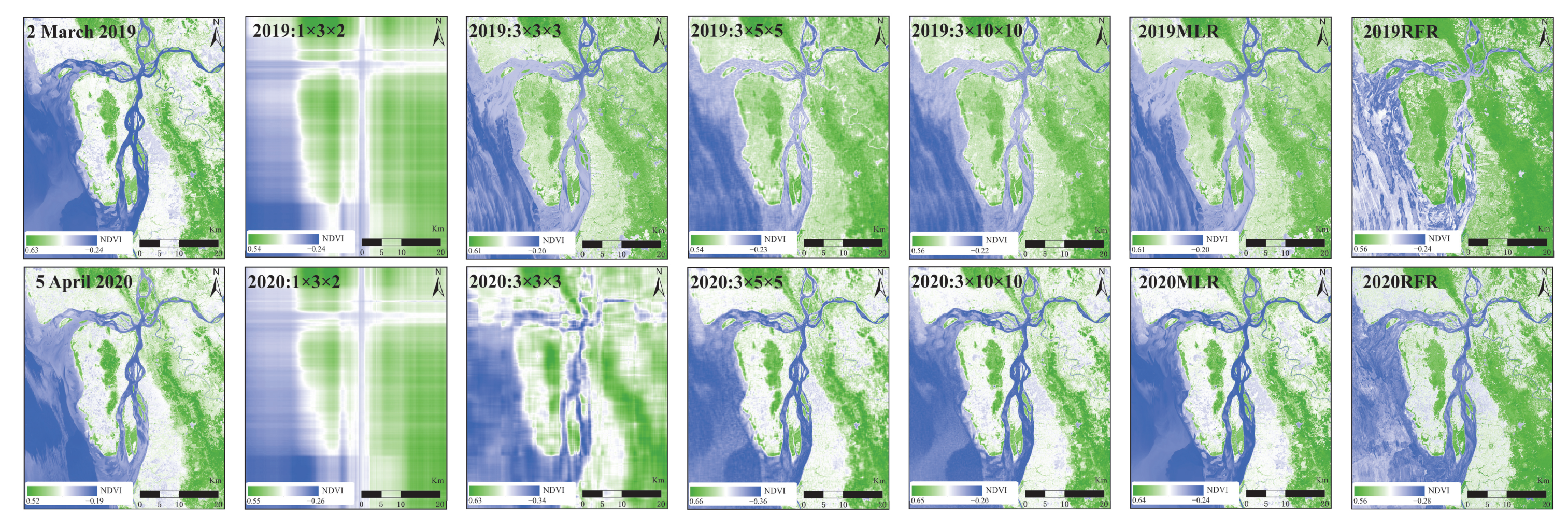
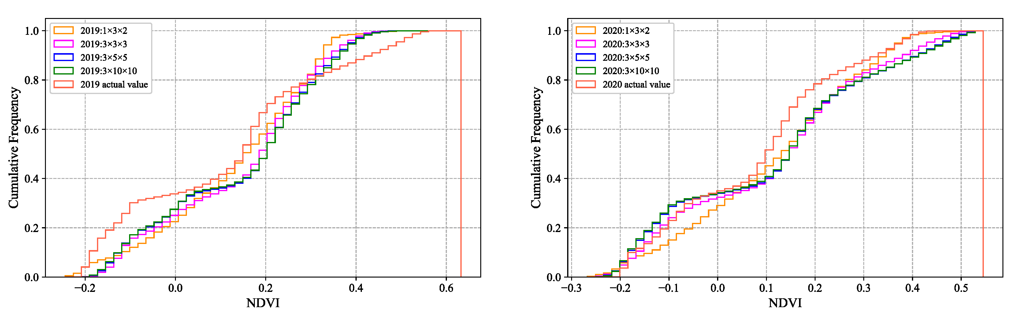
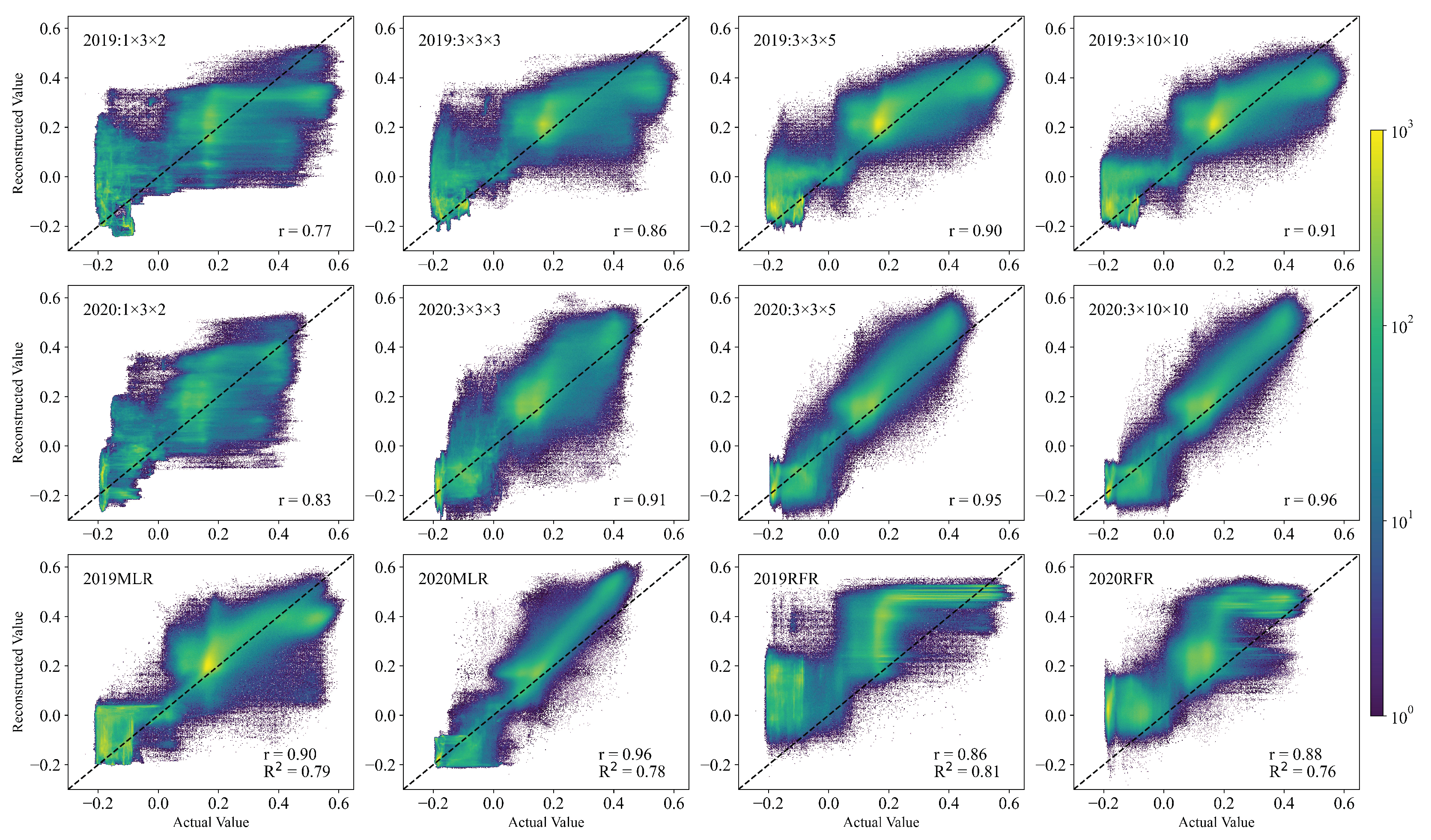
3.1. Analysis of Reconstructed Results

Reconstruction results based on different rank sizes using the proposed approach are shown in Figure 3. First, when ranks were $1\times 3\times 2$, the approximate tensor reconstructed basic topography of the study area. Second, when ranks were upgraded to $3\times 3\times 3$, topographic features were more clearly portrayed, and the trends and the detailed features of vegetation cover were clearly distinguished. For example, the darker the green areas, the higher the NDVI values, indicating that the vegetation cover was higher in these areas. Third, when ranks were increased to $3\times 5\times 5$, most vegetation-cover information in 2019 and 2020 was reconstructed and fully predicted, with RMSEs of $0.110$ for 2019 and $0.098$ for 2020, especially for the vegetation-cover characterization of offshore islands and complex water systems at the estuary. Moreover, Figure 3 demonstrates that the reconstruction results of SWTSA with rank size of $3\times 10\times 10$ were better than those of RFR, and almost the same as those of MLR. Furthermore, to explore the precision of reconstruction results, we constructed larger ranks.

Actual and reconstructed values had a similar accumulation curve (Figure 4), and more than $85\%$ of actual and reconstructed areas overlapped. Meanwhile, cumulative curves with different rank sizes implied that the larger ranks of core tensor may not mean significant improvement in accuracy for reconstruction results. According to the evaluation metrics shown in

Table 2. Performance evaluation of reconstruction.

Method	Year/Ranks	Accuracy	Precision	Recall	${\mathbf{F}}_1$ Score	Kappa
SWTSA	2019/$1\times 3\times 2$	$0.848$	$0.876$	$0.786$	$0.829$	$0.627$
	2019/$3\times 3\times 3$	$0.900$	$0.931$	$0.852$	$0.890$	$0.758$
	2019/$3\times 5\times 5$	$0.916$	$0.936$	$0.879$	$0.906$	$0.800$
	2019/$3\times 10\times 10$	$0.918$	$0.937$	$0.881$	$0.908$	$0.805$
	2020/$1\times 3\times 2$	$0.907$	$0.920$	$0.873$	$0.896$	$0.783$
	2020/$3\times 3\times 3$	$0.957$	$0.960$	$0.944$	$0.952$	$0.903$
	2020/$3\times 5\times 5$	$0.978$	$0.979$	$0.973$	$0.976$	$0.952$
	2020/$3\times 10\times 10$	$0.980$	$0.980$	$0.975$	$0.978$	$0.955$
MLR	2019/-	$0.917$	$0.930$	$0.884$	$0.906$	$0.804$
	2020/-	$0.981$	$0.981$	$0.977$	$0.979$	$0.957$
RFR	2019/-	$0.711$	$0.832$	$0.571$	$0.677$	$0.179$
	2020/-	$0.751$	$0.851$	$0.636$	$0.728$	$0.330$

, for most of the reconstruction results, values of accuracy, precision, recall, and ${\mathrm{F}}_1$ score exceeded $0.85$, which was considered to be acceptable. When rank sizes increased to $3\times 5\times 5$, the values of kappa concordance coefficient corresponding to 2019 and 2020 exceeded $0.80$ and $0.95$, respectively. In comparison with RFR, SWTSA has better accuracy and reconstruction capabilities. Moreover, Table 2 demonstrates that SWTSA and MLR had almost the same reconstruction effect corresponding to rank size of $3\times 10\times 10$.

A plot of reconstructed against actual values shows that reconstructed values were closer to actual values with an increase in the number of ranks (Figure 5). Meanwhile, for most reconstruction results, the values of Pearson’s correlation coefficient (r) exceeded $0.85$. The coefficient of determination ($R^2$) of MLR and RFR was around $0.8$, which was considered unacceptable. Further, reconstruction results for 2020 were better than those for 2019 (Figure 3, Figure 4 and Figure 5), indicating that optical remote-sensing images from the same platform (Landsat-8) may obtain different results.

Lastly, considering the execution time of the proposed algorithm and the accuracy requirements of the reconstructed results, we chose the approximate reconstruction result with ranks of $3\times 10\times 10$ for 2019, and the approximate reconstruction result with ranks of $3\times 5\times 5$ for 2020. Both RMSE values for the chosen ranks were below $0.15$ (Figure 6). All statistical indicators were consistent across results (

Table 3. Statistical characteristics of actual and reconstructed values.

Datasets	Samples	Mean	Variance	Minimum	Maximum
2019 actual value	4,030,560	$0.1203$	$0.0476$	$-0.2433$	$0.6322$
2019 SWTSA	4,030,560	$0.1349$	$0.0326$	$-0.2203$	$0.5651$
2019 MLR	4,030,560	$0.1546$	$0.0300$	$-0.2083$	$0.6020$
2019 RFR	4,030,560	$0.2925$	$0.0290$	$-0.2489$	$0.5651$
2020 actual value	4,030,560	$0.1052$	$0.0395$	$-0.1974$	$0.5109$
2020 SWTSA value	4,030,560	$0.1203$	$0.0462$	$-0.2307$	$0.5387$
2020 MLR	4,030,560	$0.1228$	$0.0480$	$-0.2401$	$0.6353$
2020 RFR	4,030,560	$0.2179$	$0.0281$	$-0.2830$	$0.5690$

).

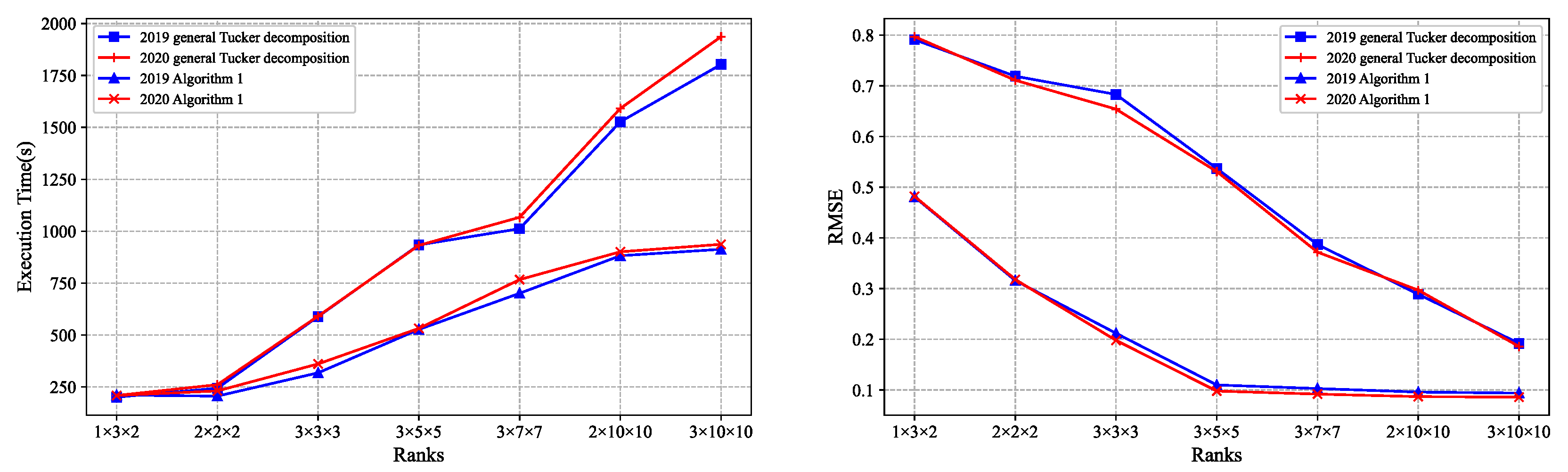
3.2. Evaluation the Performance of SWTSA

Figure 6 shows a quantitative evaluation of execution time and RMSE metrics of the proposed algorithm and the general Tucker decomposition method. First, our results showed that the proposed algorithm required less execution time and had a lower RMSE than that of the general Tucker decomposition method. Second, execution time increased with the increase in rank size. Meanwhile, the increase in execution time with Algorithm 1 was lower than that with the general Tucker decomposition method. Third, our proposed algorithm converged faster than the general Tucker decomposition method did in terms of RMSE. Additionally, the size of the core tensor influenced reconstructive results significantly. When the ranks of the core tensor increased to $3\times 5\times 5$, RMSE exhibited a trend toward convergence. Generally, RMSE values obtained with Algorithm 1 in all experiments were less than $0.5$, with the best RMSE was less than $0.1$.

The receiver operating characteristic (ROC) curves of MLR, RFR, and different rank sizes of core tensor are shown in Figure 7. The area under the curve (AUC) was also calculated to estimate the performance of SWTSA; for all reconstruction results, the values of AUC exceeded $0.9$, which showed SWTSA to be able to achieve robust performance for reconstruction.

4. Discussion

The NDVI contains important data for providing vegetation cover information and supporting environmental analyses. This article highlighted that accurately reconstructing NDVI value for cloud-covered pixels in optical remote-sensing imagery is an urgent issue in widening NDVI-based applications. The proposed approach is reliable and suitable for reconstructing outliers of NDVI from multitemporal optical remote-sensing images. This facilitates vegetation dynamic change detection and environmental analyses in cloudy areas. However, there are some limitations in this study that need to be further improved and optimized.

First, optical images used in experiments were all acquired by the Landsat series satellites. The influence of data acquired by sensors of other Earth observation plans, such as MODIS, Sentinel, and SPOT on reconstruction results needs further experimental research and analysis. Moreover, wavelengths of infrared and near-infrared bands of sensors from different periods of the Landsat series were slightly different. In this experiment, we did not consider the possible impact of this difference on results due to the inability to perform in situ spectral measurements.

There are few valid data for analysis from summer because of the majority cloudy weather in summer. Our proposed method can effectively reconstruct outliers in summer on the basis of acquired winter data. However, the impact of increasing valid data from summer on the reconstruction results remains to be assessed.

The spatial resolution of all optical images was resampled to 30 × 30 m according to the spatial resolution of the majority of images being 30 × 30 m in the dataset (Table 1). On the one hand, optical remote-sensing images with resolution higher than 30 m were difficult to obtain in the early stage. On the other hand, field measurements could not be carried out due to the impact of COVID-19. Therefore, different resolutions and coregistration errors had an unclear effect on the experimental results.

Lastly, this paper focused on exploring NDVI reconstruction methods for cloud-covered pixels on the basis of the data structure of NDVI from clear skies and their changing characteristics; therefore, reasons for long-term NDVI changes were not analyzed and discussed. In future work, we aim to quantitatively discuss the possible effects on NDVI changes that land use changes, deforestation, and riverbed evolution. Meanwhile, in order to enhance the data fusion capability of the algorithm, we aim to implement the proposed algorithm on the basis of Google Earth Engine (GEE) [52,53], a cloud computing platform, in further work.

5. Conclusions

This article presented a tensor framework for reconstructing the NDVI on the basis of tensor decomposition and a sliding-window-based reconstruction algorithm from multitemporal optical remote-sensing images. We proposed a generic algorithm and used it successfully with NDVI that was extracted from Landsat series optical remote-sensing images for an estuary of Salween River in Southeast Asia. Our results showed that the proposed algorithm was able to reconstruct NDVI with small ranks and less execution time than the general Tucker decomposition method can. Compared with RFR, SWTSA achieved better accuracy and reconstruction capabilities. Moreover, experimental results demonstrated that SWTSA and MLR had almost the same reconstruction effect corresponding to rank size $3\times 10\times 10$. Lastly, this approach was capable of describing spatial distribution patterns and temporal evolution at different levels (rank sizes). In addition, we determined that large core tensors may not mean significant improvement in accuracy for reconstruction of NDVI, but a significant increase in the execution time of the algorithm.

References

1. Forkel, M.; Carvalhais, N.; Rödenbeck, C.; Keeling, R.; Heimann, M.; Thonicke, K.; Zaehle, S.; Reichstein, M. Enhanced seasonal CO2 exchange caused by amplified plant productivity in northern ecosystems. Science 2016, 12, 696–699. [Google Scholar] [CrossRef] [PubMed] [Green Version]
2. Jia, K.; Yang, L.; Liang, S.; Xiao, Z.; Zhao, X.; Yao, Y.; Zhang, X.; Jiang, B.; Liu, D. Long-Term Global Land Surface Satellite (GLASS) Fractional Vegetation Cover Product Derived From MODIS and AVHRR Data. IEEE J. Sel. Top. Appl. Earth Observ. Remote Sens. 2019, 12, 508–518. [Google Scholar] [CrossRef]
3. Cornejo, D.; Jose, R.; Hartfield, K.; Willem, L.; Ponce, E.; Castellanos, A. Landscape Dynamics in an Iconic Watershed of Northwestern Mexico: Vegetation Condition Insights Using Landsat and PlanetScope Data. Remote Sens. 2020, 12, 2519. [Google Scholar] [CrossRef]
4. Hantson, S.; Huxman, T.E.; Kimball, S.; Randerson, J.T.; Gould E, M.L. Warming as a Driver of Vegetation Loss in the Sonoran Desert of California. J. Geophys. Res. 2021, 126, e2020JG005942. [Google Scholar] [CrossRef]
5. Lasaponara, R. Estimating Interannual Variations in Vegetated Areas of Sardinia Island Using SPOT/VEGETATION NDVI Temporal Series. IEEE Geosci. Remote Sens. Lett. 2006, 3, 481–483. [Google Scholar] [CrossRef]
6. Revuelta-Acosta, J.D.; Guerrero-Luis, E.S.; Terrazas-Rodriguez, J.E.; Gomez-Rodriguez, C.; Alcalá Perea, G. Application of Remote Sensing Tools to Assess the Land Use and Land Cover Change in Coatzacoalcos, Veracruz, Mexico. Appl. Sci. 2022, 12, 1882. [Google Scholar] [CrossRef]
7. Chiang, Y.; Chen, K. Multi-scale analysis of vegetation dynamics from satellite images. In Proceedings of the 2013 IEEE International Geoscience and Remote Sensing Symposium—IGARSS, Melbourne, Australia, 21–26 July 2013; pp. 3923–3926. [Google Scholar]
8. Bashir, B.; Cao, C.; Naeem, S.; Zamani, J.; Bo, X.; Afzal, H.; Jamal, K.; Mumtaz, F. Spatio-Temporal Vegetation Dynamic and Persistence under Climatic and Anthropogenic Factors. Remote Sens. 2020, 16, 2612. [Google Scholar] [CrossRef]
9. Ma, L.; Zhou, Y.; Chen, J. Estimation of Fractional Vegetation Cover in Semiarid Areas by Integrating Endmember Reflectance Purification Into Nonlinear Spectral Mixture Analysis. IEEE Geosci. Remote Sens. Lett. 2015, 12, 1175–1179. [Google Scholar]
10. Rodrigues, A.; Marcal, A.; Cunha, M. Monitoring Vegetation Dynamics Inferred by Satellite Data Using the PhenoSat Tool. IEEE Trans. Geosci. Remote Sens. 2013, 51, 2096–2104. [Google Scholar] [CrossRef]
11. Bignami, C.; Chini, M.; Amici, S.; Trasatti, E. Synergic Use of Multi-Sensor Satellite Data for Volcanic Hazards Monitoring: The Fogo (Cape Verde) 2014–2015 Effusive Eruption. Front. Earth Sci. 2020, 8, 22. [Google Scholar] [CrossRef] [Green Version]
12. Holmlund, K.; Grandell, J.; Schmetz, J.; Stuhlmann, R.; Bojkov, B.; Munro, R.; Lekouara, M.; Coppens, D.; Viticchie, B.; August, T.; et al. Meteosat Third Generation (MTG): Continuation and Innovation of Observations from Geostationary Orbit. Bull. Am. Meteorol. Soc. 2021, 102, 990–1015. [Google Scholar] [CrossRef]
13. Ghosh, A.; Pal N., R.; Das, J. A fuzzy rule based approach to cloud cover estimation. Remote Sens. Environ. 2006, 100, 531–549. [Google Scholar] [CrossRef]
14. Wang, Y.; Li, R.; Hu, J.; Wang, X.; Wang, Y. Evaluations of MODIS and microwave-based satellite evapotranspiration products under varied cloud conditions over east Asia forests. Remote Sens. Environ. 2021, 264, 112606. [Google Scholar] [CrossRef]
15. Domnich, M.; Sünter, I.; Trofimov, H.; Wold, O.; Harun, F.; Kostiukhin, A.; Järveoja, M.; Veske, M.; Tamm, T.; Voormansik, K.; et al. KappaMask: AI-Based Cloudmask Processor for Sentinel-2. Remote Sens. 2021, 13, 4100. [Google Scholar] [CrossRef]
16. Pablo Arroyo-Mora, J.; Kalacska, M.; Trond Løke, D.; Nicholas, C.; Coops, L.; George, L. Assessing the impact of illumination on UAV push broom hyperspectral imagery collected under various cloud cover conditions. Remote Sens. Environ. 2021, 258, 112396. [Google Scholar] [CrossRef]
17. Whitcraft, A.K.; Vermote, E.F.; Becker-Reshef, I.; Justice, C.O. Cloud cover throughout the agricultural growing season: Impacts on passive optical earth observations. Remote Sens. Environ. 2015, 156, 438–447. [Google Scholar] [CrossRef]
18. Stathopoulos, S.; Tsonis, A.; Kourtidis, K. On the cause-and-effect relations between aerosols, water vapor, and clouds over East Asia. Theor. Appl. Climatol. 2021, 144, 711–722. [Google Scholar] [CrossRef]
19. Dirk, T.; Martin, S.; Hannah, A.; Andrea, B. Investigating ESA Sentinel-2 products’ systematic cloud cover overestimation in very high-altitude areas. Remote Sens. Environ. 2021, 252, 112163. [Google Scholar]
20. Mo, Y.; Xu, Y.; Chen, H.; Zhu, S. A Review of Reconstructing Remotely Sensed Land Surface Temperature under Cloudy Conditions. Remote Sens. 2021, 13, 2838. [Google Scholar] [CrossRef]
21. Zhou, Y.; Wang, S.; Wu, T.; Feng, L.; Wu, W.; Luo, J.; Zhang, X.; Yan, N. For-backward LSTM-based missing data reconstruction for time-series Landsat images. GIsci. Remote Sens. 2022, 59, 410–430. [Google Scholar] [CrossRef]
22. Wu, P.; Yin, Z.; Yang, H.; Wu, Y.; Ma, X. Reconstructing Geostationary Satellite Land Surface Temperature Imagery Based on a Multiscale Feature Connected Convolutional Neural Network. Remote Sens. 2019, 11, 300. [Google Scholar] [CrossRef] [Green Version]
23. Zhao, W.; Duan, S. Reconstruction of daytime land surface temperatures under cloud-covered conditions using integrated MODIS/Terra land products and MSG geostationary satellite data. Remote Sens. Environ. 2020, 247, 111931. [Google Scholar] [CrossRef]
24. Zhu, Z.; Woodcock, C.E.; Holden, C.; Yang, Z.Q. Generating synthetic Landsat images based on all available Landsat data: Predicting Landsat surface reflectance at any given time. Remote Sens. Environ. 2015, 162, 67–83. [Google Scholar] [CrossRef]
25. Zhu, X.; Chen, J.; Gao, F.; Chen, X.; Masek, J.G. An enhanced spatial and temporal adaptive reflectance fusion model for complex heterogeneous regions. Remote Sens. Environ. 2010, 114, 2610–2623. [Google Scholar] [CrossRef]
26. Mutanga, O.; Adam, E.; Cho, M.A. High density biomass estimation for wetland vegetation using WorldView-2 imagery and random forest regression algorithm. Int. J. Appl. Earth Obs. Geoinf. 2012, 18, 399–406. [Google Scholar] [CrossRef]
27. Ghamisi, P.; Rasti, B.; Yokoya, N.; Wang, Q.; Hofle, B.; Bruzzone, L.; Bovolo, F.; Chi, M.; Anders, K.; Gloaguen, R.; et al. Multisource and multitemporal data fusion in remote sensing: A comprehensive review of the state-of-the-art. IEEE Geosci. Remote Sens. Mag. 2019, 7, 6–39. [Google Scholar] [CrossRef] [Green Version]
28. Qiu, Y.; Zhou, G.; Huang, Z.; Zhao, Q.; Xie, S. Efficient Tensor Robust PCA Under Hybrid Model of Tucker and Tensor Train. IEEE Signal Process Lett. 2022, 29, 627–631. [Google Scholar] [CrossRef]
29. Wu, F.; Li, Y.; Li, C.; Wu, Y. A Fast Tensor Completion Method Based on Tensor QR Decomposition and Tensor Nuclear Norm Minimization. IEEE Trans. Comput. Imaging 2021, 7, 1267–1277. [Google Scholar] [CrossRef]
30. Du, A.; Cheng, S.; Wang, L. Low-Rank Semantic Feature Reconstruction Hashing for Remote Sensing Retrieval,IEEE Geosci. Remote Sens. Lett. 2022, 19, 1–5. [Google Scholar]
31. Ludwig, M.; Morgenthal, T.; Detsch, F. Machine learning and multi-sensor based modelling of woody vegetation in the Molopo Area, South Africa. Remote Sens. Environ. 2019, 22, 195–203. [Google Scholar] [CrossRef]
32. Rouse, W.; Haas, R.; Schell, A. Monitoring Vegetation Systems in the Great Plains with ERTS. In Proceedings of the Third ERTS Symposium, Washington, DC, USA, 10–14 December 1973; pp. 309–317. [Google Scholar]
33. Yunus, A.; Fan, X.; Tang, X. Decadal vegetation succession from MODIS reveals the spatio-temporal evolution of post-seismic landsliding after the 2008 Wenchuan earthquake. Remote Sens. Environ. 2020, 236, 111476. [Google Scholar] [CrossRef]
34. Grill, G.; Lehner, B.; Thieme, M.; Geenen, B.; Tickner, D.; Antonelli, F.; Babu, S.; Borrelli, P.; Cheng, L.; Crochetiere, H.; et al. Mapping the world’s free-flowing rivers. Nature 2019, 569, 215–221. [Google Scholar] [CrossRef] [PubMed]
35. Vermote, E.; Justice, C.; Claverie, M. Preliminary analysis of the performance of the Landsat 8/OLI land surface reflectance product. Remote Sens. Environ. 2016, 185, 46–56. [Google Scholar] [CrossRef] [PubMed]
36. USGS. Available online: https://www.usgs.gov/landsat-missions/using-usgs-landsat-level-1-data-product (accessed on 8 March 2022).
37. Méger, N.; Rigotti, C.; Pothier, C. Ranking evolution maps for Satellite Image Time Series exploration: Application to crustal deformation and environmental monitoring. Data Min. Knowl. Discov. 2019, 33, 131–167. [Google Scholar] [CrossRef] [Green Version]
38. Cui, L.; Zhao, Y.; Liu, J.; Wang, H.; Han, L.; Li, J.; Sun, Z. Vegetation Coverage Prediction for the Qinling Mountains Using the CA–Markov Model. ISPRS Int. J. Geo-Inf. 2021, 10, 679. [Google Scholar] [CrossRef]
39. Geng, L.; Ma, M.; Yu, W. Validation of the MODIS NDVI Products in Different Land-Use Types Using In Situ Measurements in the Heihe River Basin. IEEE Geosci. Remote Sens. Lett. 2014, 11, 1649–1653. [Google Scholar] [CrossRef]
40. Kolda, T.; Bader, B. Tensor Decompositions and Applications. SIAM Rev. 2009, 51, 455–500. [Google Scholar] [CrossRef]
41. Hached, M.; Jbilou, K.; Koukouvinos, C.; Mitrouli, M. A Multidimensional Principal Component Analysis via the C-Product Golub–Kahan–SVD for Classification and Face Recognition. Mathematics 2021, 9, 1249. [Google Scholar] [CrossRef]
42. Sun, J.; Papadimitriou, S.; Yu, P. Window-based Tensor Analysis on High-dimensional and Multi-aspect Streams. In Proceedings of the Sixth International Conference on Data Mining, Hong Kong, China, 18–26 December 2006, ICDM’06; pp. 1076–1080.
43. Papalexakis, E.; Faloutsos, C.; Sidiropoulos, N. Tensors for Data Mining and Data Fusion: Models, Applications, and Scalable Algorithms. ACM Trans. Intell. Syst. Technol. 2016, 8, 1–44. [Google Scholar] [CrossRef] [Green Version]
44. Tucker, L. Some mathematical notes on three-mode factor analysis. Psychometrika 1966, 31, 279–311. [Google Scholar] [CrossRef]
45. Sun, J.; Tao, D.; Papadimitriou, S. Incremental tensor analysis: Theory and applications. ACM Trans. Knowl. Discov. Data 2008, 2, 1–37. [Google Scholar] [CrossRef]
46. Zhou, L.; Du, G.; Wang, R.; Tao, D.; Wang, L.; Cheng, J.; Wang, J. A tensor framework for geosensor data forecasting of significant societal events. Pattern Recognit. 2019, 88, 27–37. [Google Scholar] [CrossRef]
47. Papalexakis, E.; Sidiropoulos, N.; Bro, R. From K-Means to Higher-Way Co-Clustering: Multilinear Decomposition with Sparse Latent Factors. IEEE Trans. Signal Process. 2013, 6, 493–506. [Google Scholar] [CrossRef]
48. Ramos-Bernal, R.N.; Vázquez-Jiménez, R.; Cantú-Ramírez, C.A.; Alarcón-Paredes, A.; Alonso-Silverio, G.A.; Bruzón, A.G.; Arrogante-Funes, F.; Martín-González, F.; Novillo, C.J.; Arrogante-Funes, P. Evaluation of Conditioning Factors of Slope Instability and Continuous Change Maps in the Generation of Landslide Inventory Maps Using Machine Learning (ML) Algorithms. Remote Sens. 2021, 13, 4515. [Google Scholar] [CrossRef]
49. Jung, C.; Lee, Y.; Cho, Y.; Kim, S. A Study of Spatial Soil Moisture Estimation Using a Multiple Linear Regression Model and MODIS Land Surface Temperature Data Corrected by Conditional Merging. Remote Sens. 2017, 9, 870. [Google Scholar] [CrossRef] [Green Version]
50. Wu, Q.; Li, Z.; Yang, C.; Li, H.; Gong, L.; Guo, F. On the Scale Effect of Relationship Identification between Land Surface Temperature and 3D Landscape Pattern: The Application of Random Forest. Remote Sens. 2022, 14, 279. [Google Scholar] [CrossRef]
51. Uschmajew, A. Local convergence of the alternating least squares algorithm for canonical tensor approximation. SIAM J. Matrix Anal. Appl. 2012, 33, 639–652. [Google Scholar] [CrossRef] [Green Version]
52. Zhou, B.; Gregory S; Zhang J. Leveraging Google Earth Engine (GEE) and machine learning algorithms to incorporate in situ measurement from different times for rangelands monitoring. Remote Sens. Environ. 2020, 236, 111521. [Google Scholar] [CrossRef]
53. Qi, S.; Song, B.; Liu, C.; Gong, P.; Luo, J.; Zhang, M.; Xiong, T. Bamboo Forest Mapping in China Using the Dense Landsat 8 Image Archive and Google Earth Engine. Remote Sens. 2022, 14, 762. [Google Scholar] [CrossRef]
Figure 1. Study area location (a) DEM (b) and NDVI image series (Terrain data based on SRTM downloaded from USGS).
Applsci 12 04412 g001
Figure 2. Tensor and sliding-window-based tensor stream analysis (The process of tensor stream construction and tensor decomposition are presented in (a), and (b) shows the process of reconstructing outlier based on SWTSA. X d , W ( d , w ) and U ( i ) represent the tensor, sliding window and the factor matrix, respectively).
Applsci 12 04412 g002
Figure 3. NDVI reconstructed results for different rank sizes.
Applsci 12 04412 g003
Figure 4. Cumulative frequency distributions of NDVI for actual and reconstructed values.
Applsci 12 04412 g004
Figure 5. Scatter plots between actual and reconstructed values for different rank sizes (r: Pearson correlation coefficient, R 2 : coefficient of determination).
Applsci 12 04412 g005
Figure 6. Execution time and the RMSE values with different rank sizes of core tensor.
Applsci 12 04412 g006
Figure 7. ROC curves of SWTSA for different rank sizes (AUC: Area Under Curve).
Applsci 12 04412 g007