Article

Modeling of Geophysical Flows through GPUFLOW

Istituto Nazionale di Geofisica e Vulcanologia, Osservatorio Etneo, 95025 Catania, Italy
*
Author to whom correspondence should be addressed.
Appl. Sci. 2022, 12(9), 4395; https://doi.org/10.3390/app12094395
Submission received: 16 March 2022 / Revised: 20 April 2022 / Accepted: 25 April 2022 / Published: 27 April 2022
(This article belongs to the Section Earth Sciences)

Abstract

:
We present a new model called GPUFLOW for the modeling and simulation of geophysical flows. GPUFLOW, which is based on the cellular automaton paradigm, features a physical model for the thermal and rheological evolution of lava flows (including temperature-dependent emissivity and cooling by radiation and air convection), support for debris flows without thermal dependency, a parallel implementation on graphic processing units (GPUs), and a simpler and computationally more efficient solution to the grid bias problem. Here, we describe the physical–mathematical model implemented in GPUFLOW and estimate the influence of input data on the flow emplacement through different synthetic test cases. We also perform a validation using two real applications: a debris flow that occurred in July 2006 in the Dolomites (Italy) and the December 2018 lava flow from the Etna volcano. GPUFLOW’s reliability prediction is accomplished by fitting the simulation with the actual flow fields, obtaining average values between ~55% and 75%.

1. Introduction

Computational fluid dynamics (CFD), the art of modeling fluid flows by numerically solving the differential equations that describe their behavior, is a powerful method in the field of scientific research to expand our understanding of the physical laws of nature and how they apply to the world that surrounds us (for example, to better understand which rheological model best describes the behavior of lava flows and how this affects their emplacement), and in practical applications (e.g., for the forecasting of lava flow paths).
Land use planning and natural risk mitigation, for example, benefit from hazard maps and scenario forecasting, and CFD provides an important tool in their production: from lava flow inundation (e.g., [1]) to tsunami inundation (e.g., [2]), from river overflow flooding (e.g., [3]) to sea ice dynamics (e.g., [4]), from landslides (e.g., [5]) to lahars (e.g., [6]); the range of phenomena that can be modeled is vast; and the tools can be employed both “offline”, to determine preventative measures or to plan for short-term phenomena (e.g., [7]), as well as “online”, to adapt intervention to the evolution of the phenomenon during a long-term event (e.g., [8]).
A landslide is a mass movement that is generally triggered by intense rainfall, an earthquake, or slope cutting. One of the most hazardous types of landslide is a rapidly moving landslide (e.g., debris flow, debris avalanche, mudflow, flow slide and rock avalanche) due to its very short duration with potentially long run-out distance and massive damage to infrastructure and the population. In recent years, great advances have been made in the simulation of rapidly moving landslides using numerical models in order to forecast the flow direction, run-out distance, and velocity and to map the expected depths and area [9,10]. Numerical models for fast-moving landslides are based on various assumptions and approaches. For example, the so-called depth-integrated models assume that a landslide behaves as a liquid mixture of interacting fluids and solids (e.g., [11,12,13,14,15,16,17,18,19]). Other numerical models use the Navier–Stokes equation for motion equations [20], while others are based on the Savage–Hutter equation with different rheologies [16] or on smoothed particle hydrodynamics (SPH) to include rheologies describing the basal friction of Bingham, frictional, Voellmy, and cohesive-frictional viscous models [18]. Recently, a quasi-three-dimensional model was developed [21] that uses the Navier–Stokes equations and assumes that the sliding mass is an incompressible Newtonian fluid. In general, numerical modeling is strictly dependent on the knowledge of the rheological characteristics of the debris flow (e.g., the concentration of solid material, evolution of the mass movement, mixture density, viscosity, etc.), as well as on the properties of the soil [22,23,24,25].
Numerical modeling of lava flows has always been of great interest both for researchers contributing to the study of lava emplacement dynamics, as well as for stakeholders involved in environmental planning and the management of volcanic emergencies. Due to the high complexity of lava flow emplacement processes, numerical models necessarily adopt different simplifications and assumptions of the governing physical equations. Two kinds of lava flow models can be identified, mainly depending on the approach used, i.e., probabilistic/stochastic or deterministic. Probabilistic models provide information about the areas most likely affected by a lava flow based on multiple sets of input parameters, neglecting the temporal evolution of the flow and constraints on the thickness (e.g., [1,26,27,28]). Deterministic models can instead simulate the spatiotemporal evolution of the flow, giving detailed information about the lava front advancement velocity and the final emplacement. The aforementioned models are all two-dimensional. However, 1D and 3D models have also been developed. The main model for a 1D channelized lava flow is FLOWGO [29,30], which was recently reimplemented using Python under the name PyFLOWGO [31]. Finally, 3D codes, such as LAVASIM [32] and GPUSPH [33], provide very detailed information about the full structure of the flow dynamics, including vertical thermal structures and the interaction between melt lava and the crust. The higher modeling complexity results in slower computation times, which prevent the use of these models for lava flow hazard forecasting and assessment.
Since 2007, graphics processing units (GPUs) have evolved from video cards dedicated to the rendering of animated 3D scenes to powerful general-purpose parallel computing devices, with a growing interest in the scientific community for the acceleration of computational-intensive algorithms. Geophysical flow modeling is one field where GPUs have seen a growing number of applications [33,34,35,36,37,38].
In this paper, we introduce GPUFLOW, a 2D cellular automaton for the simulation of Bingham fluids with optional temperature-dependent rheology. GPUFLOW is an evolution of the well-established MAGFLOW lava flow model [1,38], with improvements in the completeness and generality of the physical model, optimizations in the numerical and computational aspects, and improved usability. We describe the physical–mathematical model, its parallel implementation optimized for GPU execution, and present some recent results and novel applications using both real and synthetic test cases.

2. Materials and Methods

2.1. The Physical-Mathematical Model

GPUFLOW is a 2D cellular automaton for the modeling of Bingham fluids with or without temperature-dependent rheological parameters. The computational domain is a rectangular grid covering the area of interest, divided into square cells. Each cell holds information about the local topography and the amount of fluid present in the cell; in the case of temperature-dependent rheology with phase transition (i.e., lava), the cell information also includes the temperature and heat for the fluid, as well as the amount of fluid that has solidified. The topographical information is taken from a digital surface model (DSM), with a resolution matching that of the cellular automaton. The initial conditions depend on whether a debris or lava flow is being simulated. For debris flow, it is possible to specify for each cell the amount of flowing material initially present in the cell. For lava flows, one or more cells can be marked as eruptive vents, with an associated mass flux rate (possibly varying in time), such that at the beginning of each time-step the amount of fluid in the cell is increased according to the current flux rate.
GPUFLOW uses a Moore neighborhood, so that each cell has eight neighbors (four in the cardinal direction, and four in the diagonal direction). The evolution function describes the amount of fluid flowing from one cell to a neighbor according to a steady-state solution of the Navier–Stokes equation for the motion of a Bingham fluid on an inclined plane in the case of pressure- and gravity-driven flow. Given the (possibly temperature-dependent) fluid viscosity η and yield strength Sy, the critical thickness hcr can be approximated as
h c r S y Δ z 2 + Δ x 2   ρ g ( Δ z + Δ h )
where ρ is the fluid density, g the gravity force per unit mass, ∆x the cell side length, ∆z the ground height difference (including any contribution from solidified fluid in the case of lava), and ∆h the difference in liquid height. When the difference in fluid height between the cells is higher than hcr, an amount of fluid q computed as
q = S y h c r 2 Δ x 3 η ( a 3 3 / 2 a 2 + 1 / 2 ) ,             a = h / h c r
is exchanged from the cell with a higher amount of fluid to the neighbor. The steady-state approximation is justified by the high effective viscosity of lava flows (derived from the empirical model by Giordano and Dingwell [39]) and can be considered valid for debris flow under appropriate constraints for the timestep.
In the case of temperature-dependent rheology, the heat and temperatures are updated as a weighted average between the incoming fluid and the fluid already present in the cell, and heat loss due to radiation and air convection on the surface is also computed (see Section 2.1.2). If the temperature drops below the phase transition temperature, an appropriate amount of fluid is converted into solid.

2.1.1. The Geometric Bias Resolution

A well-known issue with cellular automata is the emplacement bias due to the cell and neighborhood geometry [17,18], with the flow tending to follow the symmetry axes, leading to unnatural emplacements on a flat surface: where a circular shape would be expected, the final emplacement is a square either parallel to the cell axis when using a Moore neighborhood (i.e., including the diagonal neighbors) or rotated by half a right angle when using a von Neuman neighborhood (i.e., only including adjacent cells in the cardinal directions). Historically, these issues have been solved either by increasing the number of symmetry axes [40] or by computationally expensive and non-deterministic Monte-Carlo methods [41].
Our proposed solution is to introduce a correction factor that scales the diagonal neighbor contributions, calibrated in order to achieve a circular emplacement on a flat DSM. Specifically, the optimal value for the diagonal correction factor α was determined empirically by simulating a pillar collapsing on a flat plane and estimating the fitness between the final emplacement and a circular form, for values in the [0, 1] range, with 0 indicating no mass flux to the diagonal neighbors (thus effectively implementing a von Neumann neighborhood), and 1 indicating equal weight for all neighbors (standard Moore neighborhood). Bisection was used to refine the range, with the optimal results obtained for α = 2−6.

2.1.2. The Thermal Model

The original thermal model implemented in MAGFLOW assumed a constant emissivity value both for the molten lava and for cooled crust (generally equal to 0.9). However, recent laboratory studies have demonstrated that the emissivity increases non-linearly with cooling, revealing considerably lower values than typically assumed. In particular, analysis of ‘aa’ lava samples from the 2001 Mt. Etna eruption, over a wide range of temperatures (773 to 1373 K) and wavelengths (2.17 µm to 21.0 µm) showed that emissivity is temperature-dependent, leading to differences up to 20% in the final emplacement of the simulated lava flows [42]. In light of this study, we found an empirical relationship that links the emissivity and temperature of lava:
ε ( T ) 0.976716 + 0.0000408881   T 1.95062 · 10 7 · T 2
To take this into account, GPUFLOW introduces support for a variable emissivity model. To allow for experimentation, the coefficients can be set by the user, as with most parameters in the model.
Another improvement in the thermal model of GPUFLOW is the inclusion of the so-called “windchill” parameter that controls cooling by atmospheric convection. This introduces a cooling component proportional to the temperature difference between lava and air, with a user-controlled parameter, expressed in W/m2/K. The default value is a null coefficient, which corresponds to the assumption that heat loss due to air convection is negligible compared to radiation. In the absence of wind, a typical value for the coefficient would be ~5 W/m2/K, increasing proportionally to the square root of the wind speed [43].

2.1.3. The Input/Output Parameters

GPUFLOW simulations require a number of input parameters: the DSM of the area of interest (defining the simulation domain and resolution), a description of the physical parameters of the fluid being simulated (density, rheological parameters, thermal parameters if appropriate), and either the initial distribution of moving material (in the case of debris flow) or the location of the vents and their mass flux rates over time (in the case of lava flows). The model produces as output snapshots of the automaton state, providing information about the fluid thickness (and temperature, if appropriate) in each cell of the domain.
Details about the format of the input/output files, as well as all other information regarding the customization of the simulation, are described in Appendix A.

2.2. The GPU Implementation

The cellular automaton paradigm shows a very high degree of parallelism that makes it particularly suitable for implementation in parallel computing hardware. To allow the execution on modern parallel computing accelerators such as GPUs, the implementation is split into a host (CPU) and device (GPU) part. The host part, rewritten in C++11 in GPUFLOW, takes care of initialization, runtime management, and data output when writing the intermediate and final results, while the computational part is entirely delegated to the device code, implemented in CUDA C++ for parallel execution on NVIDIA GPUs.
The original GPU implementation of MAGFLOW already provided speed-ups of two orders of magnitude over its serial CPU counterpart [38], allowing 7-day forecasts for lava flow to be obtained in a few seconds and a month’s forecast in a few minutes. GPUFLOW introduces several optimizations to the device-side of the code, both for performance and for higher numerical robustness. Additionally, we have introduced the possibility to compile the code in a CPU-only environment, using OpenMP to distribute computations across multiple CPU cores. This allows access to the model improvements even on machines where an NVIDIA GPU is not available and allows us to provide better insight into the performance gains that can be obtained by using GPUs over CPUs.
More details about the GPU implementation of GPUFLOW and the most recent optimizations are reported in Appendix B.

3. Sensitivity Analysis

We describe the sensitivity analysis carried out on the new thermal model implemented in GPUFLOW (including the temperature-dependent emissivity and the windchill coefficient) and on the diagonal correction factor.

3.1. Impact of the Thermal Model

We performed a sensitivity analysis of the variable emissivity and the windchill included in the thermal model of GPUFLOW through different synthetic simulations. To avoid the influence due to the real rough topography, GPUFLOW simulations were run on planes with different inclinations (from 5° to 30° with 5° steps) and different constant effusion rates (10, 20, and 30 m3/s for one day), while keeping the same single vent located on the top of the plane. For the rheological properties, we used the typical parameters retrieved from literature for a’a lavas: 1360 K and 1143 K as extrusion and solidification temperatures, respectively, 2600 kg·m−3 as density, and 0.05 wt% as the water content.
The influence of constant and variable emissivity on the maximum length reached by the simulated lava flows is shown in Figure 1. In particular, we plotted the length ratios between the simulations run with a constant emissivity of 0.6 and 0.9, with respect to the simulations run with a temperature-dependent emissivity (Equation (3)), taken as reference.
Figure 2 shows the maximum lengths reached by lava flows simulated on a 20° inclined plane using constant and variable emissivity and a windchill coefficient for the cooling from 0 (heat loss due to air convection is negligible compared to radiation) to 25.

3.2. Impact of the Diagonal Correction

Evaluation of the impact of the diagonal correction factor to reduce the emplacement bias due to the cell geometry was done by simulating a debris column collapse on a flat surface. The choice to model this as a debris flow was motivated by the intent to eliminate perturbing factors, such as the mass flux rate or the temperature-dependent rheology.
The material is assumed to have a density of 2300 kg/m3 and a Bingham rheology with yield strength of 1254 Pa and a consistency index of 30.5 Pa·s. The starting condition for the collapse is with all the debris occupying a single cell, with a 4000-m-high column.
Figure 3 shows the final emplacements for different values of the diagonal correction factor. With factor 0, the flow only happens between cells in the east/west and north/south directions (Von Neumann neighborhood), resulting in the classical diamond shape. With factor 1, the flow also happens in the diagonal direction (Moore neighborhood), and the resulting emplacement preserves a square-like shape even at longer times. By contrast, the ideal coefficient value of 2−6 results in a nearly perfectly circular emplacement.

4. Results

To validate the model and test the GPU performance, we present two application results and a comparison between the runtimes of the CPU and GPU versions of GPUFLOW. The real cases include the emplacements obtained from the simulation of a debris flow that occurred in 2006 in the territory of Cortina d’Ampezzo (Dolomites, Italy) and the lava flow emitted during the December 2018 eruption of Etna volcano.

4.1. Simulation of the 2006 Debris Flow in the Territory of the Dolomites

On 5 July 2006, an intense rainstorm triggered six debris flows in the Boite River Valley, just upstream of the town of Cortina d’Ampezzo (Fiames locality, Belluno, Italy). Immediately after the 2006 event, field surveys were carried out in the study area to measure different features of the deposits [44]. Here, we present the results of the debris flow that originated from catchment 4, which produced a deposit of about 6800 m2, with a length of ~300 m and a mean sediment thickness of 1.5 m, resulting in a total volume of 11000 m3 [44].
The debris flow was simulated using the 10-m Tinitaly DEM [45] with the catchment area and the rheological properties extracted from the literature [44].
The GPUFLOW-simulated flows and the actual flow retrieved from the field survey [44] are reported in Figure 4. The simulation without a bias correction (Figure 4a) had a total length of 328 m and an extension of 28,000 m2, while the one executed with the α = 2−6 bias correction (Figure 4b) had a length of 340 m, covering an area of 24,000 m2. This provided a fitting, estimated as the square root of the ratio between the intersection and union of the simulated and actual flow fields, of 54% and 59%, respectively.

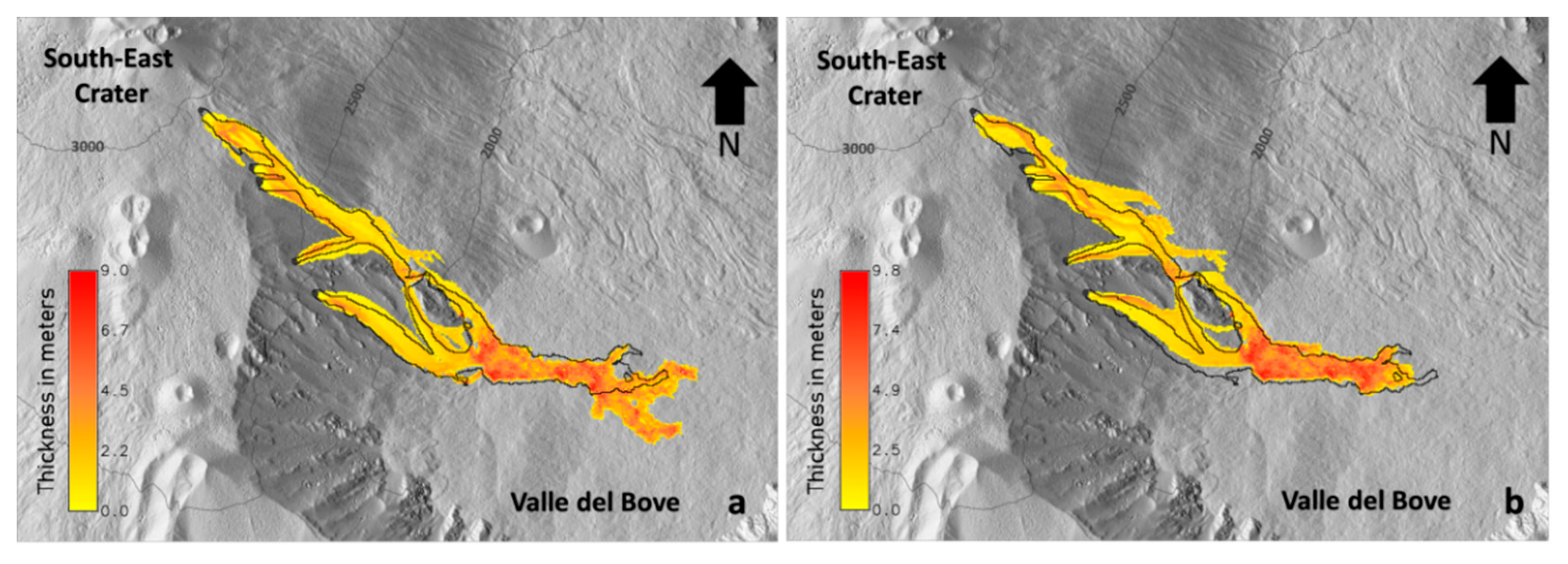
4.2. Simulation of the 2018 Etna Eruption

The December 2018 Etna eruption started from a fissure that opened on the eastern side of Etna’s South-East Crater (SEC) and propagated to the south-east, overcoming the edge of the western wall of the Valle del Bove (VdB), reaching a total length of ~2 km. The lava flow, which lasted only three days, reached a distance of about 4.2 km and covered an area of ~1 km2. The time-averaged discharge rate (TADR) and the volume were estimated by using mid- and thermal infrared data acquired by the Spinning Enhanced Visible and InfraRed Imager (SEVIRI) through the HOTSAT system [46,47].
Lava flow was simulated on a 10-m DSM of Etna that covers the summit craters and a portion of the southeastern flank of the volcano, obtained by processing tri-stereo Pléiades 1A imagery acquired on 18 July 2016 using the MicMac photogrammetric library [48]. The eruptive vents were located along the vast N–S to NW–SE fracture that opened on the upper SE flank [47]. For the rheological properties, we used the typical parameters of the Etnean lava, e.g., 1360 K and 1143 K as extrusion and solidification temperatures, respectively, 2600 kg·m−3 as density, and 0.05 wt% as the water content.
The lava flows simulated by GPUFLOW for the 2018 flank eruption are reported in Figure 5, together with the actual field retrieved from the PlanetScope image acquired at 09:19 GMT on 29 December 2018 (spatial resolution of 3 m). Lava flows were driven by using the maximum effusion rate derived from the SEVIRI data (see Figure 8 in [47]). The simulation run without the bias correction (Figure 5a) had a total length of 4.5 km and an extension of 1.35 km2, while the one executed with the α = 2−6 bias correction (Figure 5b) had a length of 4.1 km, covering an area of 1.23 km2. The fitting obtained was 74% for the simulation without the bias correction and 75% for the one with the bias correction. Refining the DSM resolution to 5 m improved the fit to 77%, at the cost of an order of magnitude longer runtime.

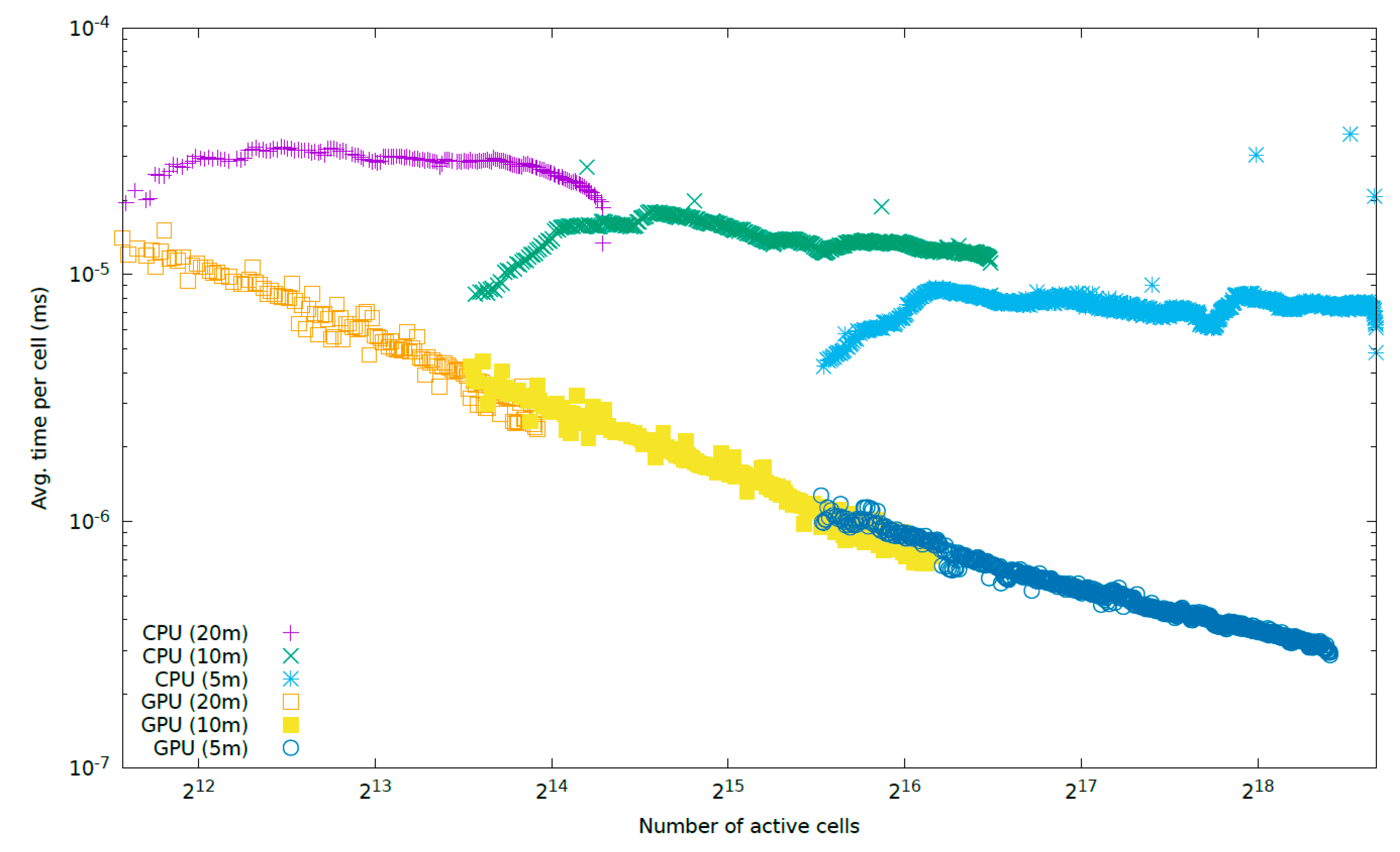
4.3. Computational Performance

To evaluate the computational performance of the model, we ran the 2018 Etna simulation at three different resolutions (5 m, 10 m, 20 m) on two different computational devices: an NVIDIA GeForce RTX 3060 GPU and an AMD Ryzen 9 5950X processor. The NVIDIA GPU features 28 computational units with a total of 3584 streaming processing elements running at 1.3 GHz, resulting in a total of approximately 10TFLOPS of single-precision processing power theoretical maximum. The AMD CPU features 16 cores (32 threads) with AVX2 support, running at 3.4 GHz with the possibility of a 4.9 GHz boost, for a total of approximately 1TFLOPS of single-precision processing power theoretical maximum.
There were minor differences in the numerical results between the CPU and GPU execution due to different degrees of accuracy of the transcendental functions, which result in slightly different numbers of active cells and enveloping region. Therefore, rather than directly comparing the full simulation runtimes, we compared the average time needed for a full iteration for a single cell, by sampling the runtime of a full iteration and dividing by the number of cells in the active region.
The results are shown in Figure 6. The GPU had a performance that was more than an order of magnitude higher than that of the 16-core/32-thread CPU in full use. The observed speed-up was consistent with the one expected from the theoretical peak TFLOPS.

5. Discussion

The physical–mathematical model included in GPFLOW provides a satisfactory description of the behavior of debris and lava flows. The variable emissivity introduced in the thermal model for lavas brings the numerical model closer to the physical phenomenon, improving the accuracy and reliability of the results. The newly introduced windchill factor can be particularly useful in nowcasting scenarios when the associated environmental factors are important. Indeed, simulations performed with a constant emissivity can deviate up to 18% in length from the simulations run with the variable emissivity (Figure 1) and up to 10% if cooling by atmospheric convection is also considered (Figure 2).
The geometric bias correction with the α parameter is fundamental to simulate debris flows, even in synthetic cases, such as a perfectly flat DSM (Figure 3), allowing us to obtain a circular emplacement instead of a square one, using a correction of 0 (i.e., no correction) or 1. This kind of correction has been proven to be particularly important for lava flow simulations, especially when the flows emplace over small slopes. Indeed, the bias correction allowed us to obtain the best fit between the simulated and real lava flow fields when it emplaced in the upper part of Valle del Bove, which has an average slope of 9.7°. Conversely, it overestimated the values for higher slopes, e.g., between 2000 and 2500 m a.s.l., where the DSM had an average slope of 28.5° (Figure 5a,b). Increasing the DSM resolution from 10 to 5 m provided better results (fitness improvement from 75% to 77%), but with an unjustified increase in computational cost. This is consistent with the results discussed in Bilotta et al. [49].
The structure of the input/output parameters introduced several benefits, with improved usability, reduced storage for simulation results, and the possibility to integrate additional features such as barriers (see Appendix A for details). All of these effects are particularly beneficial when running a large number of simulations, for example, during the creation of long-term hazard maps, where the impact of computational times and storage requirements scale with the number of simulations (in the order of hundreds of thousands).
Finally, the GPU implementation increased the execution efficiency and further speeded up the simulations, with the 2006 debris flow and the three days of the 2018 eruption performed in 2 and 3 s, respectively. From Figure 6, it is evident that, at each given resolution, the average CPU runtimes were essentially constant (independent of the growing number of active cells during the simulation), while the average GPU runtime steadily decreased. This indicates that, while the CPU was saturated (all computational resources were fully in-use during the simulation), the GPU was not, even with hundreds of thousands of active cells. This was expected since millions of work-items are needed to saturate modern GPUs. It also can be noted that even though the CPU was always saturated, an improvement in average computational runtimes was observed at higher resolution. This may be explained by the different density in actually active cells within the active region at different resolutions.
The main limitation of GPUs compared to CPUs is the fixed, limited amount of RAM. This can be worked around using a multi-GPU code [50], but on modern GPUs, this has never actually been an issue in practical applications, since GPUFLOW is normally operated at moderately low resolutions (5 m or 10 m), and even an automaton with 1 m cells spanning the 12 km × 8 km area of the central edifice of Mt Etna fit in less than 4 GB of RAM.

6. Conclusions

Mathematical modeling represents a powerful tool for forecasting the area affected by geophysical flows and assessing the associated hazard and risk. The improvements to GPUFLOW presented in this paper expand the scope of application of the model to a wider range of geophysical flows and can improve the accuracy of the simulation in many circumstances by taking into account additional factors that can affect the flow emplacement. The validation carried out on two real events, debris flow in the Dolomites and lava flow from the Etna volcano, confirmed the overall reliability of the model for these two kinds of geophysical flows and assessed the numerical robustness of its implementation.
The model is currently able to simulate debris and lava flows under specific assumptions and conditions. For example, the simulation of debris flows neglects the temperature of the material and the variation in the material composition during the event. Moreover, lava flows are subject to strong thermal effects, including phase transition, which can cause the formation of levees, crusts, and tunnels. These phenomena, which are currently not considered, are fundamental for hazard purposes, possibly impacting flow emplacement and redirecting the flow.
GPUFLOW is actively maintained and updated to introduce new features and optimizations. Future topics of research will include an automatic calibration of the geometric bias coefficient based on the local slope of the terrain. The simulation of debris flow will be validated by using other real test cases, with measured detached niches and deposits and different transported materials. Different rheological models will also be considered in order to allow GPUFLOW to cover a wider range of geophysical flows, including different types of landslides.

Author Contributions

Conceptualization, A.C. and G.B.; Data curation, A.C. and G.G.; Formal analysis, A.C. and G.B.; Funding acquisition, A.C.; Investigation, G.G.; Methodology, A.C., G.B. and G.G.; Software, G.B.; Writing—original draft, A.C., G.B. and G.G. All authors have read and agreed to the published version of the manuscript.

Funding

This work was supported by the INGV project Pianeta Dinamico (CUP D53J19000170001) funded by MIUR (“Fondo finalizzato al rilancio degli investimenti delle amministrazioni centrali dello Stato e allo sviluppo del Paese,” legge 145/2018), Tema 8–PANACEA.

Conflicts of Interest

The authors declare no conflict of interest.

Appendix A

The command-line to run GPUFLOW has the following format:
./gpuflow <dsm_file> <init_file> <vent_or_debris_file> <state> [-c] [-d output_folder] [--device X] [--debris] [--barrier barrier_file] [--diagonal-correction value]
where:
  • dsm_file is the name of the DSM representing the topography of the area of interest around the lava or debris flow; it should be large enough to cover the entire final emplacement of the flow;
  • init_file is the name of the initialization file, where most simulation settings (e.g., rheological properties of the lava) are set;
  • vent_or_debris_file is the name of the file describing the source term; this is either the location and extension of the vent(s) and/or fracture(s) in an eruption, or a DSM representing the initial distribution of movable mass in the case of a debris flow;
  • state is the name of the state file. This will be used to store the automaton state in a way that allows restarting the simulation from the given moment in time (adding the -l option to the command);
  • -c specifies compression of the output files (in.zip format);
  • -d introduces the output_folder, which is the name of the directory where all outputs pertaining the current the simulation will be stored;
  • --device specifies the GPU where the simulation will be run;
  • --debris specifies that a debris flow should be simulated (as opposed to a lava flow, which is the default);
  • --barrier includes barriers to the simulation, with the geometries specified in the barrier_file;
  • --diagonal-correction to set the diagonal correction factor to the specified value.
The DSM can be loaded as an ASCII grid (GRASS and ArcInfo formats are both supported) or as a band-sequential binary file (.bsq) with an associated ASCII header in ENVI format (.hdr) for the metadata. The binary format is preferred because it is significantly smaller (50% or more) and considerably faster to load.
The init_file is a configuration file in text format including different types of information regarding the lava or debris properties (e.g., density, emission and solidification temperature in Kelvin, emissivity, viscosity law, water content) and the simulation setup (e.g., the end of the simulation and the time step for storage, both expressed in seconds).
In the case of a lava flow simulation, the vent_or_debris_file describes the location of eruptive vents and fractures, and a reference to the flux rate file, an external text file describing the TADR as it changes over time. The syntax for the vent_file itself is a sequence of blocks, separated by an empty line, with each block in the form:
location: x_coord y_coord
temperature: lava_temperature
tstart: time_start
tend: time_end
fluxrate: fluxrate_filename
Eruptive fissures are described as a segmented line; in this case, location should include the start and end coordinates of each segment end:
location: x1_coord y1_coord x2_coord y2_coord x3_coord y3_coord ……
temperature: lava_temperature
tstart: time_start
tend: time_end
width: width_in_meters
fluxrate: fluxrate_filename
For both vents and fractures, it is also possible to specify the width, determining how many cells are activated (either around the punctiform vents or in the cross direction for each fracture segment).
All active vents and fractures during a simulation should be included in sequential order within the same vent_file. Different times in the activation/deactivation can be specified using the parameters tstart and tend.
fluxrate_filename, which is a required argument in case of a lava flow simulation, is the text file that should specify the time instant (in seconds) and the corresponding effusion rate (in cubic meters/seconds). In the case of eruptive fissure, the defined effusion rate is assumed to be distributed homogeneously along the active cells of the fracture. When different vents and/or fractures are active simultaneously, the flux rate can be divided by specifying for each of them a particular percentage through an optional numeric flux_pct parameter after the fluxrate_filename.
In the case of a landslide simulation (enabled through the --debris command-line option), vent_or_debris_file is a GIS raster file similar to the DSM (and should have the same resolution) including the detachment niche, whose 3D distribution determines the volume: each non-zero cell in the raster file will correspond to an initial corresponding height in the simulation. Negative values are allowed, indicating that a corresponding amount of mass should be subtracted from the DSM (for example, a raster value of −10 indicates that 10 m will be subtracted from the DSM and added to the flowing mass height in the corresponding cell of the automaton).
During the simulation run, different files are stored in the output_folder at a rate depending on the time step for storage specified in the init_file. Each output file is a raster file in ENVI format, cut to exactly contain the area covered by the flow, whose name includes the simulated time at the time of writing. The file stored at the end of the simulation includes the sentence “final” to be recognized (e.g., data1.21e+06-final.bsq). Each output file includes four bands for lavas: total height (liquid plus solid lava, band 1), solid height only (band 2), heat (band 3), and temperature (band 4). Optionally, it is also possible to store the per-cell maximum total (band 5) and liquid (band 6) height achieved during the simulation. In the case of debris flow, the output file includes only two bands, one with the flow thickness (band 1) and the other with the total height (soil plus flow, band 2).
In addition to the raster files, GPUFLOW stores the directory settings including all input files and the command used to run the simulation, a csv file containing all the execution times at each iteration, and three png images with the last maps of the thickness distribution, the DSM where the simulated geophysical flow has been added, and the distribution of temperatures (in the case of a lava flow).
For risk mitigation purposes, it is also possible to add barriers to a simulation. These are specified on the command line as —barrier barrier_file, where the specified file name points to a text file with a syntax similar to that of the vent file:
location: x1_coord y1_coord x2_coord y2_coord
height: height_in_meters
width: width_in_meters
where location specifies the start and end coordinates (more than two points in the case of segmented lines) of the barrier or ditch, height can be positive (in the case of barriers, added to the DSM) or negative (in the case of ditches, subtracted from the DSM), and width is the width in meters. All artificial barriers or ditches that should be considered during a simulation should be included in sequential order within the same barrier_file. This option has greatly reduced the computational times in case of volcanic emergency, where numerous simulations should be run in a limited time to evaluate how mitigation actions can affect the flow direction. Indeed, different tests can be done by automatically considering one or more artificial barriers, instead of manually manipulating the topography over which the flow emplaces.
Finally, during the run, using the commands kill -USR1 PID and kill -USR2 PID, it is possible to force the saving at the instant of execution and to print on screen the state and statistics of the running simulation (with process ID PID).

Appendix B

GPUFLOW is split into a host (CPU) and device (GPU) part, which are continuously updated. The host part is written in C++11 and handles the initialization, runtime management, and the storage of the data output. The device part is written in CUDA, which is a parallel computing platform and programming model developed by NVIDIA for general computing on graphical processing units (GPUs), and takes care of all computational aspects.
Each of the integration steps of the automaton is implemented as a separate computational kernel:
  • Erupt runs in parallel over all cells that correspond to a vent, computing the new mass and heat to be added to the cell by linear interpolation of the time-averaged discharge rate (TADR) flux rate information;
  • CalcFlux runs for every cell in the active bounding box, computing the mass and heat flux between cells as described by the physical model in 2.1 and the maximum allowed time-step for each cell;
  • Reduce computes the minimum of the allowed time-steps to be used for the update;
  • UpdateCells runs again on every cell in the active bounding box to update the new fluid and solid height, heat, and temperature of the cell from the fluxes computed by CalcFlux and Erupt.
Source information is stored in global rather than constant memory. While the source data are effectively constant during the entire simulation, the limited amount of constant memory present on GPUs caused significant management issues in the old code, requiring a rebuilding of the program in order to accommodate the correct balance between the number of active vents and the number of samples in the TADR curve. By moving the data to global memory, all the information can be allocated dynamically. Thanks to the presence of L1 and L2 caches on newer hardware generations and the use of restricted pointers, there was no measurable loss in performance introduced by the change. Constant memory is still used for all other simulation constants (DSM resolution, rheological parameters, etc.) derived from the initialization parameters.
Recent optimizations concern the data layout, including the use of a transposed launch grid, and the storage of mass and heat flux as a single two-component vector instead of two separate floating-point values.
CalcFlux is a template function, parametrized on the rheology and emissivity laws. The use of a template rather than a simple function eliminates runtime conditionals from the device runtime, improving execution efficiency. This is particularly important in the differentiation of the different rheological models supported by GPUFLOW.
Both CalcFlux and UpdateCells include optimizations to compensate for the possibility that the active region may contain potentially large numbers of inactive cells. The work-items operating in lockstep (warp of CUDA threads) on the GPU all check if the cell they are mapped to is active, and if no work-item in the warp maps to an active cell, the entire warp ends the iteration, freeing up resources for the next batch of work items.
To allow the device part to compile for CPU using OpenMP, the CUDA-specific syntax (kernel launch grid specification on the host, work-item indexing on the device) has been wrapped into appropriate C++ constructs, for which a plain C++ version mapping the kernel launches into OpenMP-parallelized for loops has also been designed. Therefore, all computational kernels use the same logic for both CPU and GPU. The only exception is the Reduce kernel, which in the CPU version is replaced by a simple OpenMP-parallelized reduction cycle. The use of a texture on GPU for the constant elevation data has been replaced on CPU with a simple linearized 2D array, with a trivial implementation of the tex2D CUDA function to access it.

References

  1. Cappello, A.; Herault, A.; Bilotta, G.; Ganci, G.; Del Negro, C. MAGFLOW: A physics-based model for the dynamics of lava-flow emplacement. Geol. Soc. Spec. Publ. 2016, 426, 357–373. [Google Scholar] [CrossRef]
  2. Weiss, R.; Munoz, A.J.; Dalrymple, R.A.; Herault, A.; Bilotta, G. Three-dimensional modeling of long-wave runup: Simulation of tsunami inundation with GPU-SPHYSICS. Coast. Eng. Proc. 2011, 32, 8. [Google Scholar] [CrossRef] [Green Version]
  3. Horritt, M.S.; Bates, P.D. Evaluation of 1D and 2D numerical models for predicting river flood inundation. J. Hydrol. 2002, 268, 87–99. [Google Scholar] [CrossRef]
  4. Rallabandi, B.; Zheng, Z.; Winton, M.; Stone, H.A. Formation of sea ice bridges in narrow straits in response to wind and water stresses. J. Geophys. Res. Ocean. 2017, 122, 5588–5610. [Google Scholar] [CrossRef]
  5. Bandara, S.; Ferrari, A.; Laloui, L. Modelling landslides in unsaturated slopes subjected to rainfall infiltration using material point method. Int. J. Numer. Anal. Methods Geomech. 2016, 40, 1358–1380. [Google Scholar] [CrossRef]
  6. Leung, M.F.; Santos, J.R.; Haimes, Y.Y. Risk modeling, assessment, and management of lahar flow threat. Risk Anal. 2003, 23, 1323–1335. [Google Scholar] [CrossRef]
  7. Zuccarello, F.; Bilotta, G.; Cappello, A.; Ganci, G. Effusion Rates on Mt. Etna and Their Influence on Lava Flow Hazard Assessment. Remote Sens. 2022, 14, 1366. [Google Scholar] [CrossRef]
  8. Cappello, A.; Ganci, G.; Calvari, S.; Perez, N.M.; Hernandez, P.A.; Silva, S.V.; Cabral, J.; Del Negro, C. Lava flow hazard modelling during the 2014–2015 Fogo eruption, Cape Verde. J. Geophys. Res. Solid Earth 2016, 121, 2290–2303. [Google Scholar] [CrossRef] [Green Version]
  9. Rickenmann, D. Empirical relationships for debris flows. Nat. Hazards 1999, 19, 47–77. [Google Scholar] [CrossRef]
  10. Crosta, G.; Cucchiaro, S.; Frattini, P. Validation of semi-empirical relationships for the definition of debris-flow behavior in granular materials. In Proceedings of the 3rd International Conference on Debris-Flow Hazards Mitigation, Davos, Switzerland, 10–12 September 2003; Millpress Science Publication: Rotterdam, The Netherlands, 2003; pp. 821–831. [Google Scholar]
  11. McDougall, S.; Hungr, O. A model for the analysis of rapid landslide motion across three-dimensional terrain. Can. Geotech. J. 2004, 41, 1084–1097. [Google Scholar] [CrossRef]
  12. Hungr, O.; McDougall, S. Two numerical models for landslide dynamic analysis. Comput. Geosci. 2009, 35, 978–992. [Google Scholar] [CrossRef]
  13. Sosio, R.; Crosta, G.B.; Hungr, O. Numerical modeling of debris avalanche propagation from collapse of volcanic edifices. Landslides 2012, 9, 315–334. [Google Scholar] [CrossRef]
  14. Pastor, M.; Blanc, T.; Haddad, B.; Petrone, S.; Sanchez Morles, M.; Drempetic, V.; Issler, D.; Crosta, G.B.; Cascini, L.; Sorbino, G.; et al. Application of a SPH depth-integrated model to landslide run-out analysis. Landslides 2014, 11, 793–812. [Google Scholar] [CrossRef] [Green Version]
  15. Wang, W.; Chen, G.Q.; Han, Z.; Zhou, S.H.; Zhang, H.; Jing, P.D. 3D numerical simulation of debris-flow motion using SPH method incorporating non-Newtonian fluid behavior. Nat. Hazards 2016, 81, 1981–1998. [Google Scholar] [CrossRef]
  16. Fernández-Nieto, E.D.; Garres-Díaz, J.; Mangeney, A.; Narbona-Reina, G. A multilayer shallow model for dry granular flows with the-rheology: Application to granular collapse on erodible beds. J. Fluid Mech. 2016, 798, 643–681. [Google Scholar] [CrossRef] [Green Version]
  17. Juez, C.; Murillo, J.; García-Navarro, P. 2D simulation of granular flow over irregular steep slopes using global and local coordinates. J. Comput. Phys. 2013, 255, 166–204. [Google Scholar] [CrossRef]
  18. Pirulli, M.; Bristeau, M.O.; Mangeney, A.; Scavia, C. The effect of the earth pressure coefficients on the runout of granular material. Environ. Model. Softw. 2007, 22, 1437–1454. [Google Scholar] [CrossRef]
  19. Savage, S.B.; Hutter, K. The motion of a finite mass of granular material down a rough incline. J. Fluid Mech. 1989, 199, 177–215. [Google Scholar] [CrossRef]
  20. Nakamura, H.; Fathani, T.F.; Karna, A.K. Analysis of land-slide debris and its hazard area prediction. In Proceedings of the International Symposium on Landslide Mitigation and Protection of Cultural and Natural Heritage, Kyoto, Japan, 21–25 January 2002; pp. 173–189. [Google Scholar]
  21. Fathani, T.F.; Legono, D.; Karnawati, D. A Numerical Model for the Analysis of Rapid Landslide Motion. Geotech. Geol. Eng. 2017, 35, 2253–2268. [Google Scholar] [CrossRef]
  22. Iverson, R.M.; Reid, M.E.; LaHusen, R.G. Debris Flow mobilization from landslides. Ann. Rev. Earth Planet. Sci. 1997, 25, 85–138. [Google Scholar] [CrossRef]
  23. Castelli, F.; Lentini, V.; Venti, A.D. Evaluation of Unsaturated Soil Properties for a Debris-Flow Simulation. Geosciences 2021, 11, 64. [Google Scholar] [CrossRef]
  24. Xu, W.J.; Dong, X.Y. Simulation and verification of landslide tsunamis using a 3D SPH-DEM coupling method. Comput. Geotech. 2021, 129, 103803. [Google Scholar] [CrossRef]
  25. Xu, W.J.; Zhang, H.Y. Research on the effect of rock content and sample size on the strength behavior of soil-rock mixture. Bull. Eng. Geol. Environ. 2021, 80, 2715–2726. [Google Scholar] [CrossRef]
  26. Felpeto, A.; Martí, J.; Ortiz, R. Automatic GIS-based system for volcanic hazard assessment. J. Volcanol. Geotherm. Res. 2007, 166, 106–116. [Google Scholar] [CrossRef]
  27. Favalli, M.; Pareschi, M.T.; Neri, A.; Isola, I. Forecasting lava flow paths by a stochastic approach. Geophys. Res. Lett. 2005, 32, L03305. [Google Scholar] [CrossRef]
  28. De’ Michieli Vitturi, M.; Tarquini, S. MrLavaLoba: A new probabilistic model for the simulation of lava flow as a settling process. J. Volcanol. Geotherm. Res. 2018, 349, 323–334. [Google Scholar] [CrossRef]
  29. Harris, A.J.L.; Rowland, S.K. FLOWGO: A kinematic thermorheological model for lava flowing in a channel. Bull. Volcanol. 2001, 63, 20–44. [Google Scholar] [CrossRef]
  30. Harris, A.; Favalli, M.; Wright, R.; Garbeil, H. Hazard assessment at Mount Etna using a hybrid lava flow inundation model and satellite-based land classification. Nat. Hazards 2011, 58, 1001–1027. [Google Scholar] [CrossRef]
  31. Chevrel, M.O.; Labroquère, J.; Harris, A.; Rowland, S. PyFLOWGO: An open-source platform for simulation of channelized lava thermo-rheological properties. Comput. Geosci. 2018, 111, 167–180. [Google Scholar] [CrossRef] [Green Version]
  32. Hidaka, M.; Goto, A.; Umino, S.; Fujita, E. VTFS project: Development of the lava flow simulation code LavaSIM with a model for three-dimensional convection, spreading, and solidification: VTFS PROJECT. Geochem. Geophys. Geosyst. 2005, 6, Q07008. [Google Scholar] [CrossRef] [Green Version]
  33. Bilotta, G.; Hérault, A.; Cappello, A.; Ganci, G.; Del Negro, C. GPUSPH: A Smoothed Particle Hydrodynamics model for the thermal and rheological evolution of lava flows. Geol. Soc. Spec. Publ. 2016, 426, 387–408. [Google Scholar] [CrossRef]
  34. Lacasta, A.; Juez, C.; Murillo, J.; García-Navarro, P. An efficient solution for hazardous geophysical flows simulation using GPUs. Comput. Geosci. 2015, 78, 63–72. [Google Scholar] [CrossRef]
  35. Juez, C.; Lacasta, A.; Murillo, J.; Garcia-Navarra, P. An efficient GPU implementation for a faster simulation of unsteady bed-load transport. J. Hydraul. Res. 2016, 54, 275–288. [Google Scholar] [CrossRef]
  36. Tafuni, A.; Domínguez, J.M.; Vacondio, R.; Crespo, A.J.C. A versatile algorithm for the treatment of open boundary conditions in Smoothed particle hydrodynamics GPU models. Comput. Methods Appl. Mech. Eng. 2018, 342, 604–624. [Google Scholar] [CrossRef]
  37. Domínguez, J.M.; Crespo, A.J.C.; Valdez-Balderas, D.; Rogers, B.D.; Gómez-Gesteira, M. New multi-GPU implementation for smoothed particle hydrodynamics on heterogeneous clusters. Comput. Phys. Commun. 2013, 184, 1848–1860. [Google Scholar] [CrossRef]
  38. Bilotta, G.; Rustico, E.; Hérault, A.; Vicari, A.; Russo, G.; Del Negro, G.; Gallo, G. Porting and optimizing MAGFLOW on CUDA. Ann. Geophys. 2011, 54, 580–591. [Google Scholar] [CrossRef]
  39. Giordano, D.; Dingwell, D.B. Viscosity of hydrous Etna basalt: Implications for Plinian-style basaltic eruptions. Bull. Volcanol. 2003, 65, 8–14. [Google Scholar] [CrossRef]
  40. Spataro, W.; Avolio, M.V.; Lupiano, V.; Trunfio, G.A.; Rongo, R.; D’Ambrosio, D. The latest release of the lava flows simulation model SCIARA: First application to Mt Etna (Italy) and solution of the anisotropic flow direction problem on an ideal surface. Procedia Comput. Sci. 2010, 1, 17–26. [Google Scholar] [CrossRef] [Green Version]
  41. Vicari, A.; Herault, A.; Del Negro, C.; Coltelli, M.; Marsella, M.; Proietti, C. Modeling of the 2001 lava flow at Etna volcano by a cellular automata approach. Environ. Model. Softw. 2007, 22, 1465–1471. [Google Scholar] [CrossRef]
  42. Rogic, N.; Bilotta, G.; Ganci, G.; Thompson, J.L.; Cappello, A.; Rymer, H.; Ramsey, M.S.; Ferrucci, F. The impact of dynamic emissivity-temperature trends on spaceborne data of the 2001 Mount Etna eruption. Remote Sens. 2022, 14, 1641. [Google Scholar] [CrossRef]
  43. Shitzer, A. Wind chill equivalent temperatures—Regarding the impact due to the variability of the environmental convective heat transfer coefficient. Int. J. Biometeorol. 2006, 50, 224–232. [Google Scholar] [CrossRef] [PubMed]
  44. Cesca, M.; D’Agostino, V. Comparison between FLO-2D and RAMMS in debris-flow modelling: A case study in the Dolomites. WIT Trans. Eng. Sci. 2008, 60, 197–206. [Google Scholar] [CrossRef] [Green Version]
  45. Tarquini, S.; Isola, I.; Favalli, M.; Battistini, A. TINITALY, a Digital Elevation Model of Italy with a 10 Meters Cell Size; Version 1.0; Istituto Nazionale di Geofisica e Vulcanologia (INGV): Roma, Italy, 2007. [Google Scholar] [CrossRef]
  46. Ganci, G.; Bilotta, G.; Cappello, A.; Hérault, A.; Del Negro, C. HOTSAT: A multiplatform system for the satellite thermal monitoring of volcanic activity. In Detecting Modelling and Responding to Effusive Eruptions; Harris, A., de Groeve, T., Garel, F., Carn, S.A., Eds.; Geological Society: London, UK, 2016; p. 426. [Google Scholar]
  47. Calvari, S.; Bilotta, G.; Bonaccorso, A.; Caltabiano, T.; Cappello, A.; Corradino, C.; Del Negro, C.; Ganci, G.; Neri, M.; Pecora, E.; et al. The VEI 2 Christmas 2018 Etna eruption: A small but intense eruptive event or the starting phase of a larger one? Remote Sens. 2020, 12, 905. [Google Scholar] [CrossRef] [Green Version]
  48. Ganci, G.; Cappello, A.; Zago, V.; Bilotta, G.; Hérault, A.; Del Negro, C. 3D Lava flow mapping of the 17–25 May 2016 Etna eruption using tri-stereo optical satellite data. Ann. Geophys. 2019, 62, VO220. [Google Scholar] [CrossRef]
  49. Bilotta, G.; Cappello, A.; Hérault, A.; Del Negro, C. Influence of topographic data uncertainties and model resolution on the numerical simulation of lava flows. Environ. Model. Softw. 2019, 112, 1–15. [Google Scholar] [CrossRef]
  50. Rustico, E.; Bilotta, G.; Hérault, A.; Del Negro, C.; Gallo, G. Scalable multi-gpu implementation of the MAGFLOW simulator. Ann. Geophys. 2011, 54, 5. [Google Scholar] [CrossRef]
Figure 1. Length ratio of the lava flows simulated with a constant emissivity of 0.6 and 0.9 vs. variable emissivity, by varying the effusion rate (a) and the inclination of the plane used as DSM (b).
Applsci 12 04395 g001
Figure 2. Trend of the maximum lengths of the lava flows simulated on a 20-degrees inclined plane using different windchill coefficients (from 0 to 25). Results were also obtained using a constant emissivity of 0.6 and 0.9 and a variable emissivity. The three downward trends were approximated by linear functions with slopes of about −14 (for 0.9 and variable emissivity) and −19 (for 0.6 emissivity).
Applsci 12 04395 g002
Figure 3. Simulation of a debris flow by collapse on a plane by using a diagonal bias correction of 0 (a), 1 (b) and 2−6 (c). Colors represent the flow thickness in meters.
Applsci 12 04395 g003
Figure 4. GPUFLOW simulations of the 2006 debris flow in the Dolomites without (a) and with (b) the bias correction. Colors represent the deposit thickness in meters. The actual debris field was redrawn from [44].
Applsci 12 04395 g004
Figure 5. GPUFLOW simulations for the 24–27 December 2018 eruption of the Etna volcano. Lava flows were simulated using the temperature-dependent emissivity without (a) and with (b) the bias correction. Colors represent the lava flow thickness in meters. The actual lava flow field extracted by the Planetscope image (area of ~1 km2) and the five emission points along the eruptive fissure is highlighted in black. The outline of the actual field was determined by adaptive local thresholding using the free and open-source GRASS GIS software.
Applsci 12 04395 g005
Figure 6. Average time (in ms) needed for a full iteration for a single cell. Simulations were run using the CPU and GPU versions of GPUFLOW at different resolutions (5, 10, and 20 m).
Applsci 12 04395 g006
Publisher’s Note: MDPI stays neutral with regard to jurisdictional claims in published maps and institutional affiliations.

