IoT System for Detecting the Condition of Rotating Machines Based on Acoustic Signals

Featured Application

The proposed system is designed for the estimation of a rotating machine’s condition, based on the acoustic signal that the machine generates. According to the information provided by this system, it is possible to plan preventive maintenance of a specific rotary machine more reliably. This system can be applied in any industrial plant with rotating machines with fixed rotational frequency.

Abstract

Modern predictive maintenance techniques have been significantly improved with the development of Industrial Internet of Things solutions which have enabled easier collection and analysis of various data. Artificial intelligence-based algorithms in combination with modular interconnected architecture of sensors, devices and servers, have resulted in the development of intelligent maintenance systems which outperform most traditional machine maintenance approaches. In this paper, a novel acoustic-based IoT system for condition detection of rotating machines is proposed. The IoT device designed for this purpose is mobile and inexpensive and the algorithm developed for condition detection consists of a combination of discrete wavelet transform and neural networks, while a genetic algorithm is used to tune the necessary hyperparameters. The performance of this system has been tested in a real industrial setting, on different rotating machines, in an environment with strong acoustic pollution. The results show high accuracy of the algorithm, with an average F1 score of around 0.99 with tuned hyperparameters.

1. Introduction

Predictive maintenance (PdM) is a well-known paradigm in machine maintenance in which the machine is observed through the available measurements and its health is estimated as well as a potential need for repair [1,2]. It is well known that the probability of failure of all machines increases with time due to component wear [3]. In this situation, it is crucial to perform timely maintenance because the replacement of worn components can increase the lifetime of the machine significantly. One of the major areas of interest of industrial predictive maintenance is the state estimation of rotary machines [4]. Therefore, it is desirable to design a system that can assess the condition of different types of such machinery.

PdM techniques for rotary machines can be generally divided into model-based and data-driven methods [2]. Model-based approaches require a priori knowledge of a system model that is often not easy to determine [2]. Nevertheless, such techniques can be very powerful and their accuracy can be improved by online estimation of model parameters. Guo et al. developed a mathematical model of the tube-ball mill and used the Genetic algorithm (GA) for online model parameters’ update in order to enhance condition monitoring of such system [5]. On the other hand, in the data-driven approaches, the necessary process information is extracted directly from a large number of recorded signals [2]. These methods usually use some statistical signal processing method to extract useful information from measurements and a machine-learning algorithm to obtain prediction results [1]. For instance, Goyal et al. developed a method with PCA analysis of vibration data and the k-nearest neighbor (KNN) classifier for diagnosing the bearing defects [6]. Saha et al. used Fourier transform (FFT) to extract the features and support vector machines (SVM) to diagnose bearing faults [7]. Other techniques such as partial least squares (PLS) [8], extreme learning machine (ELM) [9] and learning vector quantization (LVQ) [10] are also successfully used for predictive maintenance and fault detection purposes. With the rise of deep learning research, this area gained even more attention. Multilayer neural networks (MNN) were used by Iannace et al. to detect an imbalance in the quadrotor’s propeller [11], while Kolar et al. in [12] utilizes a deep neural network (DNN) for AC motor state monitoring and tests the influence of the number of kernels on classification result.

Due to their diversity, all these available solutions tend to be specialized for a specific type of rotary machines such as rolling element bearings [13], mills [14], turbines [15], and so forth. Solutions that can be adjusted to a wide range of problems are usually quite expensive, require a number of sensor elements and processors, and are often tied to specific industry manufacturers. Although vibration sensors are traditionally used in PdM systems [16] for rotary machines, the use of acoustic sensors should be considered due to their low cost and contactless acquisition. The acoustic signals are more susceptible to noise than vibration signals, but they have also proven effective in the state estimation [17,18,19]. This potential is additionally explored throughout this paper.

On the other hand, with the development of Industry 4.0 and Industrial Internet of Things (IoT) paradigm, predictive maintenance strategies have become more popular than ever [3]. IoT architecture enables various devices with sensors to communicate with each other and/or with a remote computer system through the Internet. Therefore, data collection and analysis became much easier, which is crucial for proper predictive maintenance and implementation of intelligent PdM methods [20]. Many IoT solutions are available in the literature for monitoring parameters of specific machines [21,22], but, to the best of the authors’ knowledge, there are no solutions that detect the condition of machines with different rotary frequencies and characteristic spectral parameters based on acoustic signals and using intelligent PdM methods.

In this paper, we propose an IoT device that (i) due to inexpensive hardware is accessible to both large industrial plants and small businesses; (ii) contains an AI state detection algorithm that can easily be adapted to a wide range of rotating machines; (iii) uses acoustic signals and can therefore acquire measurements in a contactless manner; (iv) can be connected to available cloud platforms; and (v) the signals are processed immediately after acquisition on the device, so no external computer is required for decision-making process. In addition, we have improved the existing state detection algorithm and designed the appropriate software for end-users. Compared to the [14,19], the state detection algorithm is upgraded using GA for optimization of neural network architecture, which makes it easily applicable to a wide range of rotary machines with different rotating frequencies. Compared to available PdM methods that are mainly focused on a specific type of rotary machine, the approach in this paper is of particular interest to all types of rotary machines with a fixed rotating frequency that experience structural changes over time. One type of such machine is a grinding mill, in which the grinding plates are gradually degraded during the grinding process. The proposed solution was tested on several coal grinding mills with fixed rotational frequencies and different dominant spectral components, located in the thermal plant. It showed very good performance in such a real industrial setting with a strong stationary acoustic noise.

This paper is structured as follows. In Section 2 the condition detection algorithm implemented on the proposed portable device is described, firstly by describing the two main approaches used for this purpose, namely discrete wavelet transform (DWT) and neural networks (NN). Then the entire algorithm is presented in detail, as well as the software developed for parameter training and hyperparameter tuning using genetic algorithms. The proposed architecture of the system is described in Section 3 with special attention given to the hardware configuration and communication paradigm. Experimental results are presented in Section 4, while Section 5 concludes the paper.

2. Condition Detection Algorithm

In order to develop a portable device capable of detecting the state of various rotary machines, it is necessary to develop an algorithm that considers the characteristic properties of acoustic signals obtained from such machines. Because rotary machines have characteristic acoustic and vibrational signatures, namely distinct peaks on typical frequencies and their higher harmonics, the problem becomes how to extract useful information in the frequency domain that can easily be adjusted to different characteristic frequencies of different machines.

The algorithm for acoustic-based rotary machine state detection presented in this paper is named FASTER (fault and state detection of rotary machineries) algorithm. It was designed bearing in mind two main objectives: (i) it needed to be easily generalizable for a wide range of rotary machines with a fixed rotational frequency; and (ii) it needed to be computationally inexpensive so that it can be implemented in real-time at microprocessor platform with modest performance. In order to provide both seemingly contradictory requests, the algorithm needs to consider the characteristic rotary acoustic signatures, as well as hardware feature performance. As was initially proposed in [19], a combination of discrete wavelet transform and simple neural networks provides an ideal solution to this problem.

2.1. Discrete Wavelet Transform

The most important step in many classification problems is the extraction of features, which will be used later as a classifier input. Features are useful information in the recorded signals that can be used to distinguish different states of machines. There are several solutions offered in the literature for feature extraction with the purpose of state detection. Most of them concentrate on detecting the frequencies of the highest peaks and the amplitudes of those peaks [23]. In order to implement feature extraction procedures such as these, it is necessary to have knowledge beforehand of what the expected spectrum of the acoustic signal looks like. Therefore, generalization for different machines with different signatures is not an easy task. Another approach is to implement some sort of filter bank with adjustable boundaries that would be applied to the signals, and descriptors such as signal power or a number of peaks can be extracted from filtered outputs. Discrete wavelet transform offers a variation of such a method, and it has been demonstrated to yield promising results for feature extraction for the purpose of machine state estimation [19].

Wavelet transform (WT) is similar to short-term Fourier transform, but instead of using windowed sinusoidal functions as the basis, WT uses wavelets, which are oscillatory signals limited in time with an average value of zero. Wavelet transform of a signal x(t), t ∈ R is defined as

$$X_{WT}\left(s,\tau \right)=\frac{1}{\sqrt{\left|s\right|}}{{\displaystyle \int }}_{-\infty }^{\infty }x\left(t\right)\psi \left(\frac{t-\tau }{s}\right)dt,$$

(1)

where $\psi \left(t\right)$ is a continuous basis function called a mother wavelet [24], $\tau \in R$ represents a time shift and $s\in R$ is a scaling factor used to scale mother wavelet. In this way, WT provides adjustable time-frequency resolution by changing the position (with parameter $\tau$) and width (with parameter $s$) of the basis $\psi \left(t\right)$. The most commonly used mother wavelet is Daubechies 4-tap, which will also be used in this paper [24]. It is worth mentioning, however, that depending on the type of wavelet $\psi \left(t\right)$, the features of the transform may differ. By adopting a discrete scaling factor $s=2^j, j=1,2,\dots$ and discrete time shift $\tau =2^{j}m, m=1,2,\dots$ a Discrete Wavelet Transform of a discrete signal $x\left(n\right), n\in Z$ is obtained, and its analytical description is

$$X_{DWT}\left(j,m\right)=\frac{1}{\sqrt{2^j}}{\displaystyle \sum }_{\mathrm{n}=-\infty }^{\infty }x\left(n\right)\psi \left(\frac{n-2^{j}m}{2^j}\right).$$

(2)

It has been shown that multiresolution can be used to obtain DWT by applying a series of low-pass (LP) and high-pass (HP) filters and downsampling the output of those filters by 2 after each step, as shown in Figure 1. In this cascading filter scheme, the output of the low-pass filter is used as an input to subsequent low-pass and high-pass filters, and this is repeated $M$ times. If $N$ is the length of the original input signal $x\left(n\right)$, then the maximum number of decomposition steps is $M_{max}={\log }_{2}N$. The outputs of each high pass filter are named detailed coefficients of the appropriate level, and outputs of the last lowpass filter are named the approximation coefficients. The total number of output samples is the same as the length of the original signal, and the parameters of the filters themselves depend on the choice of the wavelet function $\psi \left(n\right)$.

The frequency band which corresponds to each level coefficient from Figure 1 is given in

Table 1. Frequency band and number of samples of coefficients for M DWT decomposition levels.

Coefficients	No. of Samples	Frequency Band
$d_1$	$\frac{N}{2}$	$\left[\frac{F_N}{2},F_N\right]$
$d_2$	$\frac{N}{4}$	$\left[\frac{F_N}{4},\frac{F_N}{2}\right]$
…	…	…
$d_{\mathrm{M}}$	$\frac{N}{2^M}$	$\left[\frac{F_N}{2^M},\frac{F_N}{2^{M-1}}\right]$
$a_{\mathrm{M}}$	$\frac{N}{2^M}$	$\left[0,\frac{F_N}{2^M}\right]$

($F_N$ denotes the Nyquist frequency of the signal). Every decomposition level in DWT yields information about a specific frequency band. The frequencies of interest can be analyzed by adjusting the parameter $M$.

This kind of multiresolution analysis is ideal for acoustic and vibrational signals of rotary machines because frequency bands can be adjusted (by manipulating parameters $M$ and $F_N$) so that each band consists of one or more characteristic frequencies. Therefore, the information about the changes at these frequencies can be extracted by calculating the power of each coefficient. This will be used later as the feature input to the classifier. Having this in mind, the first objective of the algorithm is fulfilled, and feature extraction can be conducted to be easily adjustable to different types of rotary machines. The second objective of the algorithm is fast implementation, and DWT is ideal for this purpose as well. The filtering scheme from Figure 1 can be implemented using the algorithm called fast wavelet transform, which is computationally inexpensive and can be used in real-time applications [25].

2.2. Neural Networks

It is well known in the machine learning community that if the features are informative enough, the classifier does not need to be complex in order to reach right decision. If the features are power values of coefficients from Table 1, the main requirement the classifier needs to fulfill is to be computationally simple and easily support various levels of problem complexity. Therefore, NN are the ideal choice because they have been shown to work both on state estimation problems [26] and when implementation on inexpensive processors is required [27].

In this paper, we used the multilayer neural network, whose structure is shown in Figure 2. The MNN consists of $K-1$ hidden layers and one output layer. The DWT power coefficients are used as input into the MNN, while the MNN output represents the estimated state of the machine. The kth layer consists of $N^k$ neurons and the output of each neuron is:

$$a_i^k={\sigma }^k\left({\displaystyle \sum }_{i=j}^{N^{k-1}}{w}_{j,i}^k{a}_j^{k-1}+b_i^k\right),i=1,\dots ,N^k,$$

(3)

where $w_{j,i}^k, j=1,\dots ,N^{k-1}$ and $b_i^k$ are the weighting coefficients and bias of ith neuron, whereas $N^{k-1}$ is the number of neurons in (k − 1)th layer. The activation function is denoted by ${\sigma }^k$, which is nonlinear if the neuron belongs to the hidden layer and linear if the neuron belongs to the output layer.

The weighting coefficients and the biases of the neural network are “trained” in such a way as to minimize the following cost function:

$$J={\displaystyle \sum }{\left(x_i-y_i\right)}^2,$$

(4)

where $x_i$ is the targeted output, and $y_i$ is the output predicted by MNN. In this paper, the Levenberg-Marquardt based backpropagation algorithm is used for training, in which the information is propagated to the network in a backward manner in order to adjust the weights and minimize the cost function [28].

In addition to the neural network coefficients (parameters) optimization, it is important to adequately choose the number of neural network layers K and the number of neurons in each layer $N^k,k=0,\dots ,K-1$ (hyperparameters).

2.3. FASTER Algorithm

The algorithm for state detection of rotary machines using acoustical signals (FASTER algorithm) is designed to run on an IoT device which consists of commercially available CPU, such as Raspberry Pi. It is based on combination of DWT for feature extraction and NN for classification, as suggested in [19]. However, since it needs to operate in real time on acoustic signals, which are at least a couple of minutes long and usually quite noisy, some additional steps need to be conducted. The entire algorithm is given in Figure 3 and parameters/hyperparameters used to adjust the algorithm for specific rotary machine are indicated.

The steps in the procedure are given as follows.

(1) Acoustic signal acquisition: The recording of the acoustic signal is obtained using an inexpensive commercially available microphone attached to the platform described in the next section. The length of the recording should be significantly longer than the length of an analyzed audio signal (L). Experimental results indicate that it should not be shorter than 5 min.

(2) Preprocessing: In this step, the recorded signal is divided into segments that have a uniform design. Therefore, the extracted features will be comparable between several recordings of different lengths. The recorded signal is windowed into smaller segments of L seconds, and the shift between two consecutive windows is d seconds. In this way, one long recording is divided into several shorter ones, which are separately analyzed. In this step, the amplitude normalization is performed as well as decimation in which the original sampling frequency is reduced to the new sampling frequency $F_s$.

(3) Feature extraction: DWT is performed on each segment from the previous step. The number of levels of DWT transform is adjusted with hyperparameter dwt_lvl, and it should be chosen to the obtained frequency bands corresponding to the machine’s rotational frequencies characteristics. After performing DWT in this way, dwt_lvl+1 different coefficients are obtained. The features are powers of these coefficients, so each segment of the length L has a total of dwt_lvl+1 features, which depend on the frequency characteristics of the signals.

(4) Classification: Neural networks are used for classification. There are dwt_lvl+1 inputs (features from the previous step) and 1 output. The output of the classifier is the decision on the state of the rotary machine, and it is a number between 1 and 4. If the output is equal to 1, it means that machine parts are healthy. The output of 2 indicates that the machine begins to wear, without a significant effect on the performance. The output equal to 3 means that the machine parts are starting to wear noticeably, but the machine still operates properly. Output equal to 4 signifies that the performance of the machine is starting to suffer, and it is necessary to perform maintenance and replace worn parts of the machine. The complexity of the neural network is described with the vector hyperparameter nn_layers. The number of vector elements determines the number of hidden layers of the network, and each element represents the number of nodes in the appropriate layer. Since it is assumed that the NN is already trained, for the classifier to be able to function properly, the information about network coefficients is provided with the parameter nn_coefficients.

The performance of the proposed condition detection algorithm depicted in Figure 3 is dependent on the described hyperparameters (L, d, Fs, dwt_lvl, nn_layers) as well as the parameters of an already trained NN (nn_coefficients). The training procedure as well as the choice of hyperparameters is conducted separately when a sufficient number of recordings is acquired.

2.4. Hyperparameter Tuning

The number of hyperparameters needed for the algorithm in Figure 3 is significant (4 different scalar values and one vector), and it is not feasible to expect the user to be able to determine the appropriate values for each machine. Therefore, some form of hyperparameter tuning algorithm needs to be developed.

Hyperparameter tuning consists of several steps: selection of the initial hyperparameters, training NN for selected values, evaluating the performance of that NN and then repeating the procedure with slightly changed values of hyperparameters. This procedure repeats several times until satisfactory results are obtained. Generally, this procedure is conducted either by trial-and-error approach or by using the grid search optimization technique. However, due to a sheer number of hyperparameters that need to be adjusted in FASTER algorithm, these approaches are too computationally expensive and calculations can last for several hours.

In this paper, the combination of heuristic rules and genetic algorithms is used for hyperparameter optimization. There is some flexibility in choosing hyperparameters used in the preprocessing step of the algorithm, so their value can be approximately determined without the need for mathematical optimization. For example, acoustic signatures for most rotary machines have significant frequencies somewhere between 1 Hz and 1000 Hz. Consequently, by choosing an audio signal whose length ($L$) is between 45 s and 60 s, the main oscillatory dynamic of the signal will be captured. The shift between two consecutive windows ($d$) should be small enough to create as many-windowed signals as possible, but large enough to keep the diversity of the recording and prevent overfitting. The choice between L/10 and L/3 is shown to be valid for all machines experimentally tested. Finally, the new sampling frequency should be several times larger than the highest significant frequency of the signal. Since most rotary machines tested within our research have the largest significant frequency of 500 Hz, the initial choice for this parameter for most industrial applications can be around $Fs=4800 \mathrm{Hz}$.

Feature extraction and classification steps of the algorithm have hyperparameters that must be adjusted more rigorously because the slightest shift in these parameters can significantly affect the overall performance. For this purpose, a genetic algorithm is used [29]. This is an optimization technique that models evolutionary theory by generating a population where individuals compete for survival. Each individual in the generation is a possible solution to a given problem (a point in the search space) and is represented by a chromosome (which is usually a set of bits). The fittest individuals (ones that are most successful by the given criteria) survive longer and reproduce, thus preserving their genetic material in the following generations. This approach is shown to work well for NN hyperparameter tuning [30] and is chosen as a promising solution for the optimization of these parameters for several reasons. First, both dwt_lvl and elements of nn_layers are integers with narrow lower and upper bounds. Therefore, this can be described as a nonlinear constrained integer optimization problem, which is challenging for many classical optimization techniques. Furthermore, an analytic solution for this problem is not possible and there are likely many local minima, so the GA approach where the entire parameter space is searched in parallel has a larger probability of finding the global solution. Finally, the performance of the trained neural network is used as an optimization criteria function, so it is stochastic in nature. GA is shown to be superior to standard optimization techniques in all these cases. A detailed description of these steps is given in Figure 4.

2.5. Configuration Software

The main feature of the IoT system proposed in this paper is ability to operate on a wide range of rotary machines. Therefore, the hyperparameters from Figure 3 need to be adjusted for each machine separately. In addition, NN must be trained for each machine as well. In order to help the end user with configuration for a specific machine, we developed a separate software application using Matlab 2018a Application Designer, and whose execution flow is given in Figure 4. The main window of this configuration software application is shown in Figure 5. Hyperparameter configuration can be manually entered in the upper left side of the window while audio signals for NN training can be loaded on the upper right side. There is an option for users to activate the hyperparameter tuning algorithm, or to select manually entered hyperparameters. Then, the neural network can be trained, and the configuration file can be generated by pressing appropriate buttons. This configuration file should be loaded into the proposed IoT system.

Before the configuration file is loaded, the portable device (described in detail in the next section) serves only for recording audio signals. These recordings are used for training the NN. When enough signals have been acquired, they are loaded into configuration software, and the corresponding real state of the machine is entered next to each signal, as shown in Figure 6 (left). When hyperparameters are adjusted and NN training completes, the performance graph is generated, as shown in Figure 6 (right). If the user is not satisfied with the performance, another NN training can be performed or can load a different set of recordings.

When the user is satisfied with the NN performance, the configuration file should be generated. This file (FASTER_config.mat) contains all the parameters and hyperparameters that must be transferred to the portable device, in order to be configured for that specific type of the machine.

3. Architecture of the Proposed System

The system we present in this paper is designed to autonomously perform an estimation of the state of the rotary machine and provide the result in a convenient way to the various stakeholders. The schematic diagram of this system is shown in Figure 7. A microphone, connected to a microprocessor platform for acquisition and processing, captures the acoustic signal produced by a rotary machine. After the recording of the acoustic signal sample is completed, its processing is performed (as explained in the previous section) in order to estimate the condition of the observed machine. The obtained result is delivered to the users.

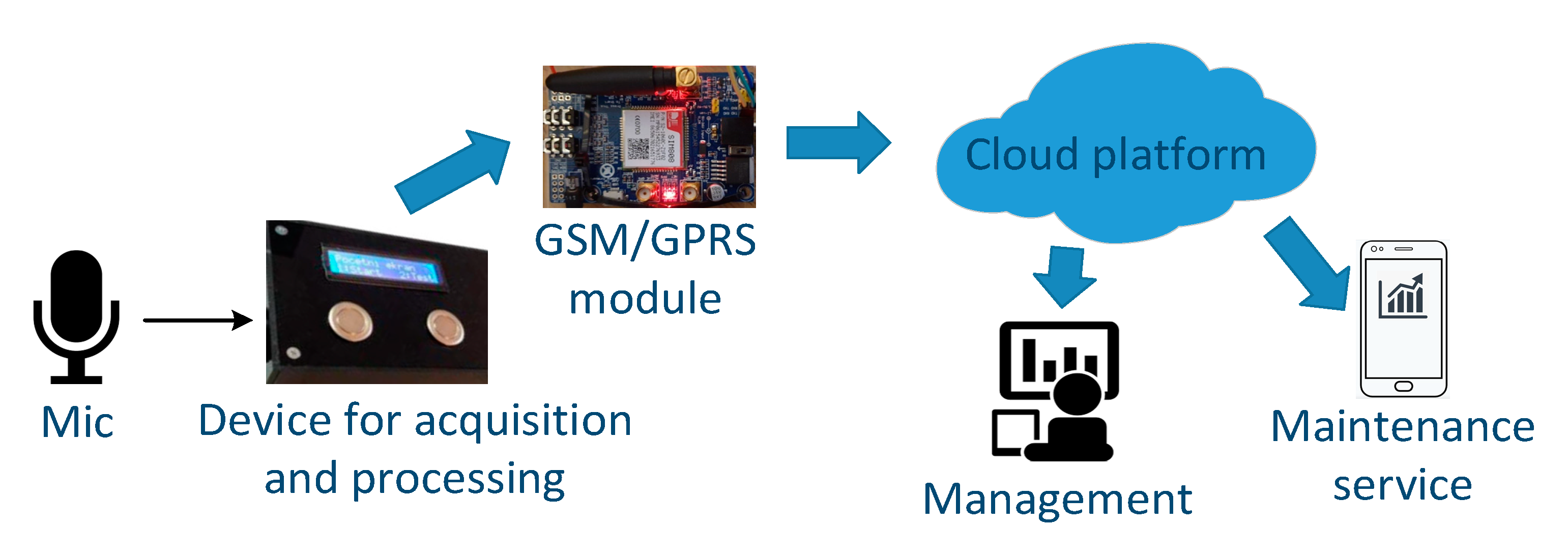
There are several interested parties for information on the current state of the rotary machine. First, it is the staff in charge of maintaining the machines. However, the management of the organization may also be interested in order to better organize and plan further activities and costs of the company. That is why we decided to send the data on the state of the machine to the cloud platform immediately after obtaining the results. In this way, we ensure the immediate availability of information to all stakeholders, regardless of where they are currently located. It is enough for them to have an Internet access and a suitable device (computer, tablet, mobile phone…) to access the cloud platform and stored data.

For the needs of this prototype, we used a cloud platform developed at the University of Montenegro, which is located on its hosts [31]. In addition to enabling data storage, this platform also enables the visualization of stored data, so that it is easier to follow the trends in the behavior of the observed machine. Usage of this platform is currently completely free. It is just necessary to register with a valid email address.

However, the data transfer between the estimating device located on the observed machine and the cloud platform is not always completely reliable. Namely, it is possible that the Internet access service provider does not work during some period. In addition, interruption of the mobile operator signal through which we establish a GPRS connection is possible. Finally, there may be a problem with the GPRS modem or the SIM card. For this reason, information about the results of signal processing and estimation of the machine state is displayed on the LCD screen, so that the operator instantly has information about the result. Moreover, the recording is stored on the SD memory card of the device, so it is possible to repeat the process of audio signal processing later and get an estimation of the machine state at the time of recording.

3.1. Hardware Implementation

The device we present in this paper is intended to work in an industrial environment and therefore must meet a number of conditions. First, it must be as small as possible, resistant to adverse working conditions in the environment, autonomous, portable, easy to install and use, and a modest consumer of electricity.

A small and light device would take up little space and interfere less with the usual working environment around a rotating machine whose condition it needs to estimate. Since this is mostly an estimation of the industrial machines, working and ambient conditions are often unsuitable for the operation of electronic devices. The presence of abrasive substances and dust, exposure to low and high temperatures, as well as their rapid changes, the danger of mechanical influences caused by force majeure or insufficient attention of the operator, cause the designed device must have a high dose of resistance and protection from these influences.

A device of this type and purpose is usually designed to be used on different machines, so it must be easily portable and autonomous in its work. This means that it must also have an autonomous power supply that will ensure long enough operation between two battery charges. Finally, since the device is portable, it is necessary that its installation and commissioning be simple so that it can be performed by a less skilled user.

After the initial consideration of the most suitable platform for the realization of the device for acoustic signal acquisition and processing, we decided to use the Raspberry Pi (RPi) platform [32]. First, it provides sufficient processing power to perform the required tasks. In addition, unlike many microcontroller platforms, it works like a regular computer with an operating system, which significantly facilitates software development, integration of hardware components and shortens the time required for implementation. Last, but not least, for our specific application, it allows easy utilization of large storage space.

Namely, acoustic signal recording produces relatively large files that need to be recorded somewhere for possibly later processing. If we also want to keep earlier recordings for comparisons and later additional analyzes, the requirements for storage space are growing rapidly. Managing such files is an additional challenge if we do not have operating system support.

RPi uses an SD memory card as a storage device. It provides space for an operating system with all the available software applications. It also uses the same memory card to store files that are the result of the user’s work. There are several supported operating systems, but in our implementation, we used Raspberry Pi OS (formerly called Raspbian) [33], which is a scaled-down version of the Linux operating system, adapted to run on RPi. The Raspberry Pi OS with desktop and recommended software takes up just under 4 GB on the memory card, but the need for space grows with the installation of additional software applications and tools. That is why we used a 32 GB memory card in our implementation. It turned out that this memory capacity is enough to install all the necessary programs and tools, as well as to store recordings from a number of acquisitions.

Acquisition of the acoustic signal is performed using a small and affordable commercial microphone, model AK5371, which connects to the microprocessor platform via a USB port. The quality of the microphone certainly affects the quality of the recording, and thus the quality of the obtained information about the condition of the machine. However, in the initial phase of the research, we found that with the help of a small, portable and affordable microphone, as we use in our system, we could get quite relevant results [34]. An additional advantage of the used microphone is a built-in A/D converter, which further facilitates its integration into the system.

During the development of the device and its initial commissioning for testing purposes, it was necessary to achieve a simple and efficient interaction between the device and the user. In order to make sure that the device works properly in certain phases of operation, the simplest way was to display certain messages to the user. An LCD screen commonly used in industrial applications has been used for this purpose. This LCD is easy to manage through the I2C communication interface, it is a small energy consumer and it is possible to display enough information.

On the other hand, the control of the device in order to issue the appropriate commands is performed by means of two buttons, also intended for industrial applications. This means that they are resistant to dust, moisture, abrasives and similar potential hazards that can be encountered in an industrial plant. With these buttons, the user navigates through the application menu, and starts or stops certain tasks.

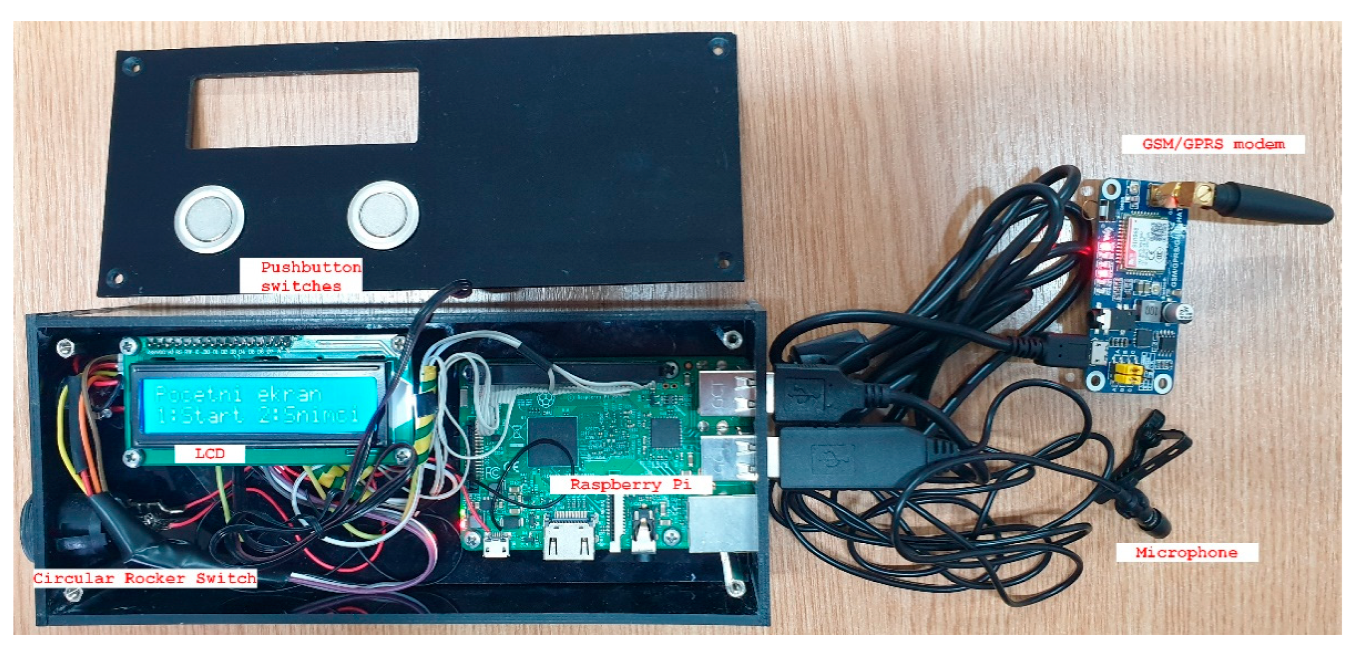
Components of the device for acoustic signal acquisition and processing and their layout in practical implementation are shown in Figure 8. Only the power bank and SD card are not visible. SD card is inserted at the bottom of the Raspberry Pi, and the power bank is accommodated at the bottom of the box, under the plastic divider that separates the power supply and electronics. The list of components used for the implementation of this device, together with the most important characteristics and approximate price, is shown in

Table 2. Specification of components used for the design of the portable device from Figure 8.

Component	Specification	Price (Approx.)
Raspberry Pi 3 Model B+	Broadcom BCM2837B0, Cortex-A53 (ARMv8) 64-bit SoC @ 1.4 GHz; 1 GB LPDDR2 SDRAM; 2.4 GHz and 5 GHz IEEE 802.11.b/g/n/ac wireless LAN; extended 40-pin GPIO header; 4 USB 2.0 ports	40 €
SD card	32 GB, micro SD card Class 10	6 €
Xiaomi 10000 18 W Fast Charge Power Bank 3	10,000 mAh, 18 W, output: 5 V-2.4 A, Max. dim. (L × W × H): 15 × 7.5 × 1.9 cm; weight 225 g	15 €
Microphone AK5371 USB 2	SNR 84 dB; frequency response: 20 Hz–16 KHz; sampling rate supported: 8 KH, 11 KHz, 11 KHz, 44 KHz, 11 KHz, 48 KHz, 16-bit stereo; sensitivity: −30 dB ± 3 dB; 16-bit A/D converter; USB interface, cable length 1.5 m	30 €
GSM-GPRS modem Waveshare GSM/GPRS/GNSS HAT	Standard Raspberry Pi 40PIN GPIO extension header, supports Raspberry Pi series boards; supports SMS, phone call, GPRS, DTMF, HTTP, FTP, MMS, email, etc. Control via AT commands; USB connection	40 €
LCD	16 character × 2 lines; 5 × 8 dots; single power supply (5 V ± 10%); I2C interface	5 €
Pushbutton Momentary Switches	MCS1901, 48 V/125 mA, vandal-proof, Ø19 mm	2 × 10 €
Circular Rocker Switch	Rating 10 A 250 V AC, insulation resistance DC 500 V 100 MΩ Min, IP65, Ø20, 2 mm	3 €

.

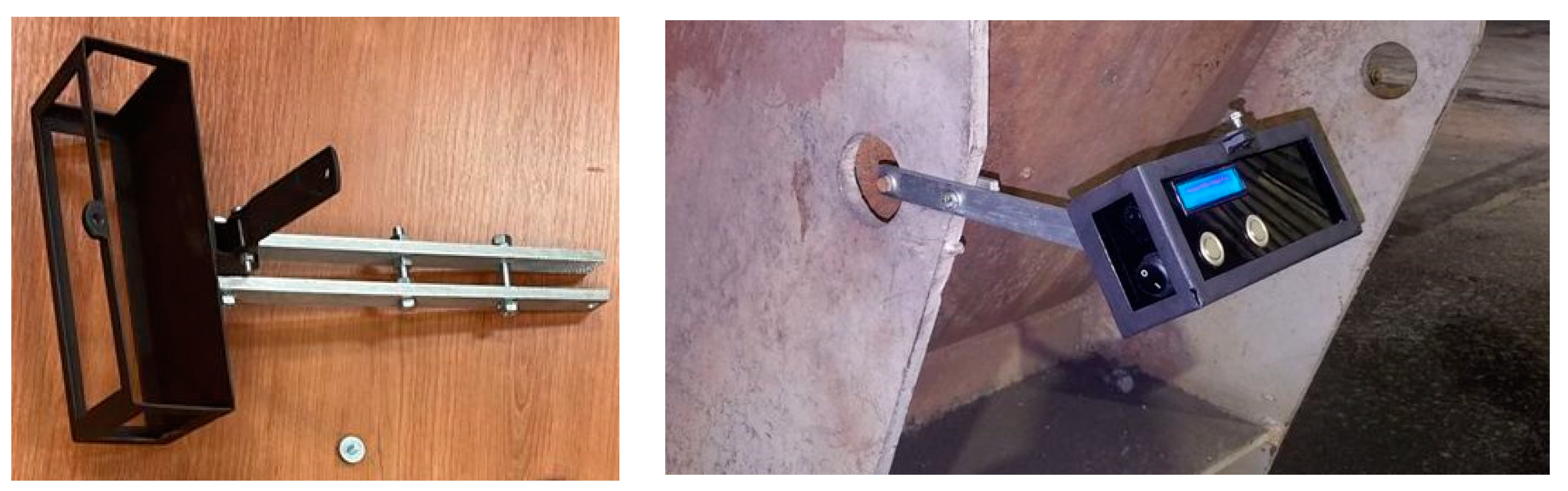
The device (the mentioned components) is packed in a plastic box, 3D printed of high-quality plastic, resistant to the high temperatures. Initially, it was planned to mount the device on the rotary machine using strong magnets. However, after the experience in the initial design phase, we gave up on such a solution because it turned out that we would have huge problems with the temperature and vibrations that produce rotary machines in an industrial surrounding. Therefore, we decided to mount the device on the machine using the bracket made of metal construction (Figure 9, left), which is fixed to the construction of the machine by the screws (Figure 9, right). Using a rod of appropriate length, which is mounted on the body of the bracket, the microphone approaches very close to the surface of the machine, while the device itself is far enough to avoid the heat impact to the body of the box and electronic components inside.

The application that runs on the Raspberry Pi is written in the Python programming language including some of the publicly available libraries. Some of them are: RPi.GPIO (for operations with general purpose input/output ports), PyAudio (for operations with audio signals and files), NumPy (for working with arrays and numerical calculations). This application starts when the operating system is booted, that is when the device is turned on. In the development and testing phase of the device, the application works by offering the user a choice between acquiring a new acoustic signal and processing already recorded acoustic signals in the form of audio files.

If the user selects the acquisition of a new audio signal, the recording of the signal captured by the connected microphone begins. The PyAudio library [35] is used for recording, which can be used to easily record and play audio signals on various platforms, including the Raspbian operating system. Recording is performed with a frequency of 48 kHz and a resolution of 16 bits. The duration of the recording is limited to five minutes, and in the processing phase it is software-wise divided into smaller pieces, more suitable for processing.

Since the device for acquisition and signal processing should work in industrial conditions, where it is not always easy to bring the power from the public grid to this device, a power bank is used as the power supply. Most of the device’s components are small consumers of electricity. However, one of the components is the GSM/GPRS module, which sends the data to the cloud. During the activation of this module, it is necessary to provide a current of close to 2 A, which is a limiting condition for choosing an adequate power source. In our prototype, we use a Xiaomi Power Bank 3 [36], which contains a Li-polymer battery with a capacity of 10,000 mAh. Our device is powered via a USB-A port of a power bank that delivers 5.1 V and provides 2.4 A.

3.2. Communication between Device for Acquisition and Cloud Platform

As mentioned earlier, the communication between the acquisition device and the cloud platform is an important segment of the proposed system. In the initial phase of development, there was a dilemma whether to transfer recorded files and perform processing on the cloud (or at the user’s server) or should perform all processing on the acquisition device and send only the obtained estimation of the machine state. Based on the experience regarding the size of the recorded files and considering the characteristics of the GPRS connection, we decided to apply this second approach [37]. Thus, the amount of data transmitted over the GPRS connection is very small, which reduces the possibility of communication problems, as well as its costs. On the other hand, reliability increases because information about the state of the machine can be obtained immediately, on the spot, even if the communication with the cloud platform does not work properly.

In the implementation of the proposed system prototype, we used the GSM/GPRS communication module Waveshare GSM/GPRS/GNSS HAT [38]. This module is adapted for use with RPi microcomputers, which greatly facilitates system development. It can be connected to RPi in several ways, and in the current implementation, a USB connection is used. RPi 3B has four USB ports available, and our device requires two: one for microphone connection and the other for a GPRS module (see Figure 8).

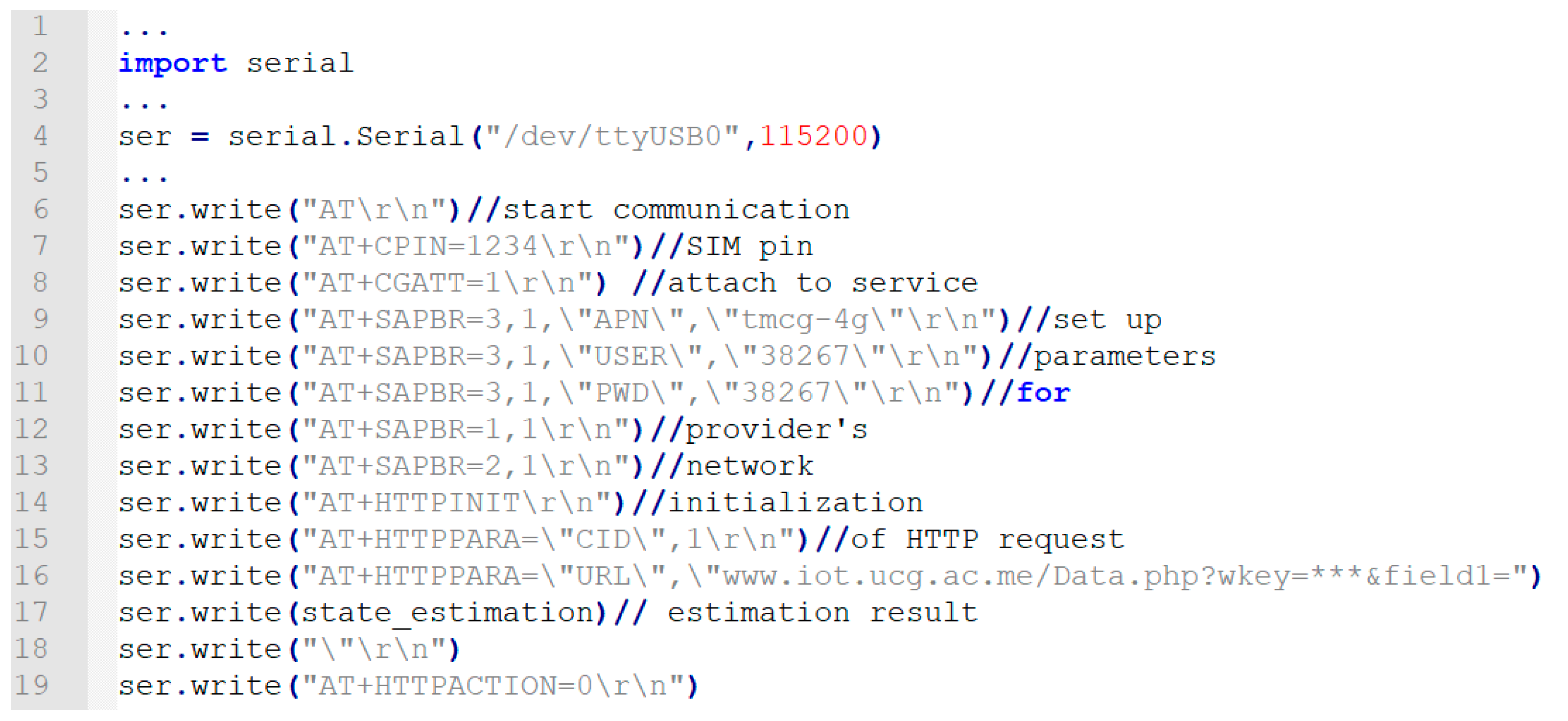
Using the USB port makes it much easier to establish communication with the GPRS module. The programmer just needs to include the serial library in the Python code (line 2 in Figure 10). After that, the communication with the corresponding device has to be opened and the communication speed is set. Then, the corresponding AT commands in the form of strings are sent to the module via a set of “write” commands.

Figure 10 shows a part of the program code for sending data about the state of the observed machine to the mentioned cloud portal. The parameters shown (apn, username, and password) refer to the local mobile Internet provider. Instead of the asterisks in line 16, the proper key for writing to the particular node of the cloud platform must be entered. Information on the estimated machine state is in the variable state_estimation. We send this information to the cloud using the GET method. This process begins with the command in line 14 by the initialization of the HTTP request and is finalized with the command in line 19.

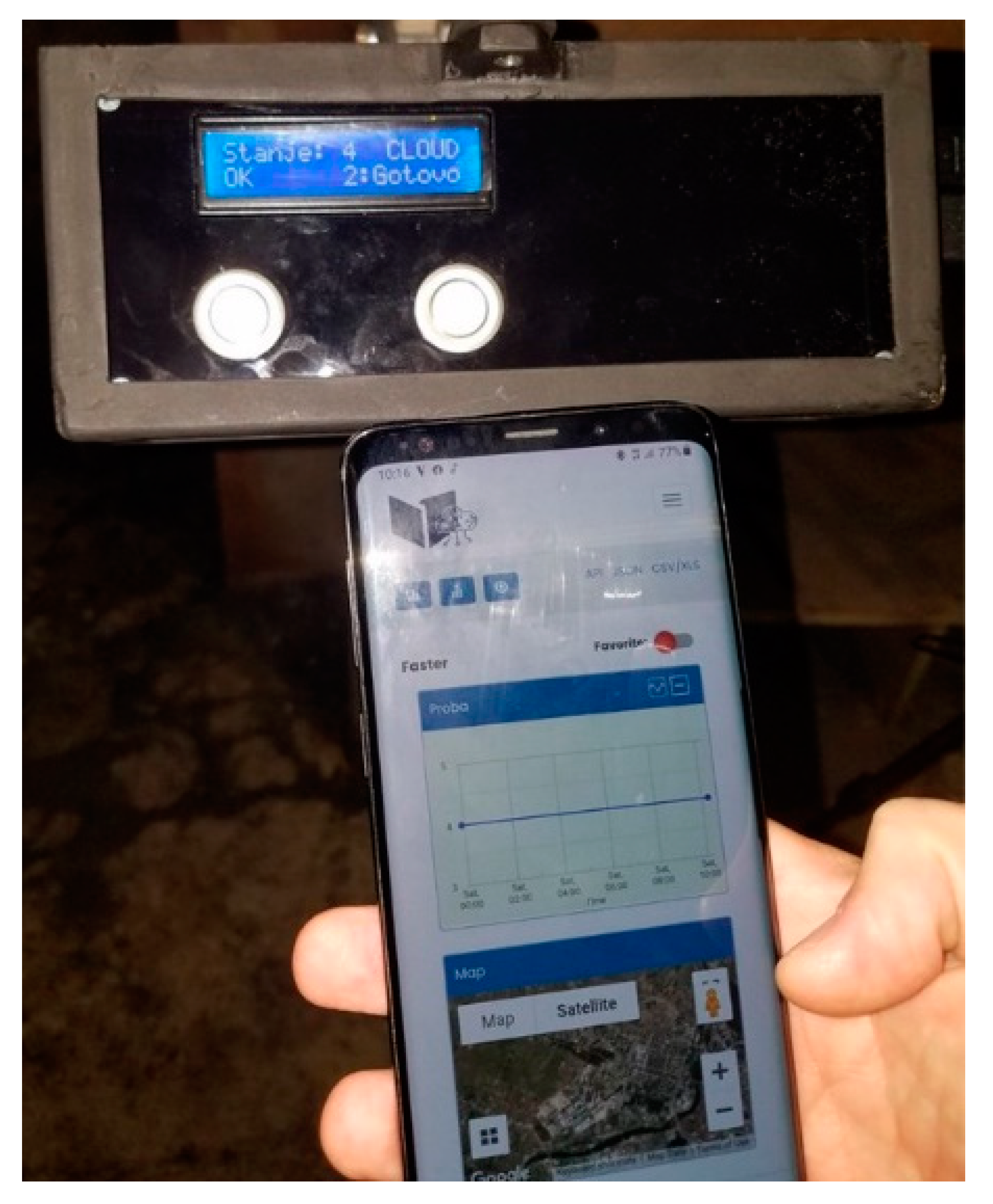
Figure 11 illustrates a diagram from a cloud platform that depicts information about the state of a rotating machine. As one can see from the figure, this diagram, and thus the information about the condition of the machine, can be downloaded and viewed by any device with Internet access, even on a mobile phone.

4. Experimental Results

The performance of the algorithm is tested in real industrial conditions, on the coal grinding mills in thermal power plants. The ability of the device to detect the rotary machine state is verified using several performance metrics. In order to demonstrate this, let us analyze in detail how the algorithm behaves on a specific coal grinding mill in a thermal power plant, previously described in [14]. The following results are obtained using Matlab 2018a on a PC with Intel Core i5-9400 CPU and 8 GB of RAM, with Windows 10 operating system. The signals are recorded with the device described in the previous section.

4.1. Coal Grinding Mill

The reason why the coal mills are chosen for verification of this IoT device is based on several factors. Firstly, the environment in which they operate is filled with significant ambient noise [18] and demonstrating that the state detection algorithm is functional in such conditions is crucial for the applicability of the proposed device. Furthermore, depending on the size of the industrial coal grinding system and construction parameters of the mill itself, the dominant frequencies in the acoustic specter of the mill can vary, simulating the diversity of acoustic signatures of different rotary machines.

Coal grinding mills are widely used in thermal power plants for the purpose of pulverizing chunks of coal into small powder, which can then be easily transferred to the burner system. Fan mills, on which we mostly concentrate in this paper, have several impact plates within the housing of the mill. The impact plates rotate around the center, and the friction between the plates and the coal causes pulverization. This effect is most efficient when the mill has been serviced and the impeller with the plates is new. With time, however, the impact plates get worn and their efficiency decreases. Generally, new grinding plates last around 60 working days in the mill, but that time can vary significantly depending on the load of the mill and the quality of coal. Therefore, a condition detection algorithm will be applied to this machine for the purpose of detecting the amount of wear on the impact plates of the mill.

Figure 12 depicts the coal grinding mill itself (left), with the motor that rotates impact plates in front of it. The schematic of its cross-section is shown in Figure 12 (right). This particular mill has a rotary frequency of 12.5 Hz, it has 10 impact plates rotating around the center, and the microphone is located on the side of the machine, close to the movement of the plates. Therefore, the frequency of the plate’s movement next to the microphone is 125 Hz. These are dominant frequencies in the specter and considering the appearance of their higher harmonics and the possibility of a slight variation of the base rotary frequency, the informative frequency bandwidth is between 10 Hz and 500 Hz. The recording sampling frequency is 48 kHz with a 16-bit resolution. Taking this into account, the preprocessing parameters are defined as $L=45 \mathrm{s}, d=15 \mathrm{s}, F_s=4800 \mathrm{Hz}$.

4.2. Preliminary Results without Hyperparameter Tuning

For initial analysis, the hyperparameter tuning step will be omitted and feature extraction and classification parameters will be set bearing in mind the complexity of the problem and the nature of acoustic signals. By adopting $dwt\_lwl=6$, 7 different DWT coefficients are generated, and the frequency bandwidth of each coefficient can be determined from Table 1. Figure 13 illustrates how the recorded signal looks in the frequency domain, on lower frequencies (up to 500 Hz) with corresponding DWT coefficients. One important thing that is worth mentioning is that the main rotary frequency of the mill (which is 12.5 Hz) is lower than the passband frequency of the microphone as stated in Table 2. For that reason, the spectral component which corresponds to this frequency is significantly weakened and the amplitude of its first harmonic (at the frequency of 25 Hz) is actually more pronounced, as can be seen in Figure 13. This means that although one of the dominant frequencies of the rotary mill is lower than the passband of the microphone, the information that this component yield is not lost since it can be captured in its higher harmonics.

By analyzing the frequency characteristics of the signal, it is clear that the most informative dynamic of the signal is captured with coefficients $a_6$ and $d_5$. Here, level 5 detail coefficients ($d_5$) contain frequencies between 75 and 150 Hz, while approximate coefficients ($a_6$) contain frequencies from 0 to 37.5 Hz, thus yielding the information about the basic rotary frequency of the mill and one higher harmonic. The power of each coefficient is used as a feature, so there are seven inputs to the NN classification algorithm. This means that the structure of the network does not need to be complex (furthermore, the complex structure can result in overfitting). Therefore, a neural network with two hidden layers and five neurons in each layer is selected ($nn\_layers=\left[5,5\right]$).

With these hyperparameters, the neural network is trained using recordings several minutes long for each of the appointed classification outputs, resulting in over 30 min worth of audio signals recorded in the period of two months. These recordings reflected all the appointed states of the particular rotary machine. Choosing the so-called ground truth (i.e., which of the four classes corresponds to each of the recorded signals) was challenging and was conducted with the help of the site operators. Namely, recordings that are obtained less than a week before the maintenance was conducted are denoted as class four recordings (i.e., they reflect extremely worn impact plates of the mill), whereas the recordings obtained in the first two weeks after the maintenance are denoted as class 1 recordings (reflecting completely healthy machine components). Class 2 roughly corresponds to recordings obtained between 2 and 4 weeks after the maintenance, while class 3 corresponds to recordings obtained around five weeks after the maintenance. It is important to mention that ground truth information about classes is always best when obtained with the input of the domain expert, and it should be carefully chosen for each rotary machine for which the algorithm is used.

When initial segmentation of recordings is conducted using the proposed hyperparameters, the training set consisted of a total of 638 samples in a 7-dimensional feature space. Out of these, 134 correspond to class 1, 190 to class 2, 188 to class 3, and 126 to class 4. The training set is divided into training segments (80%) and validation segments (20%). After the training of the neural network is conducted, the testing is performed on new recordings which were previously not seen by the network. The total number of testing samples is 295 (64 from class 1, 82 from class 2, 74 from class 3, and 75 from class 4), and the resulting confusion matrix is shown in

Table 3. Confusion matrix for fixed hyperparameter classification.

		PREDICTED
		1	2	3	4
ACTUAL	1	64	0	0	0
	2	0	82	0	0
	3	0	3	64	7
	4	0	0	2	73

. Since the diagonal entries correspond to the correct classification, the accuracy of the algorithm (the number of correctly classified samples divided by a total number of samples) is $acc=0.96$.

It is important to verify that the classification procedure is able to correctly generalize the results and that the high accuracy achieved in this example is not accidental. For that reason, the training and testing of the neural network was repeated in order to validate the behavior of the algorithm. All the data from the previous example (the total of 933 samples) was again randomly divided into training (70%) and testing (30%) sets and this partitioning was conducted four times, simulating a form of cross-validation verification. The results are presented using boxplot visualization in Figure 14, where each train-test partitioning is shown in different color. For each class, classification results are presented with median value (denoted with circles) and 25th and 75th percentile (denoted with horizontal lines). It is evident that high classification accuracy is achieved with all data partitions which shows that overfitting has not occurred and the algorithm performs properly.

The nature of state detection problem and the requirements of the experts from maintenance teams indicates that the classification errors are not equally significant. Classes 1, 2, and 3 correspond to the proper functioning of the machine, indicating how soon the machine maintenance will be required. This helps about planning regular maintenance, but does not signal the need for immediate response and replacement of worn parts. Class 4, on the other hand, alarms that the maintenance needs to be performed. For that reason, it is of crucial importance to determine reliably if machine operates in class 4 regime, while misclassification between classes 1, 2, and 3 does not substantially affect maintenance performing.

This means that it is worth to examine the algorithm behavior with respect to class 4, apart from accuracy which is a metric that describes overall functioning of the algorithm. If class 4 is denoted as positive, and classes 1, 2, and 3 as negative, then the new confusion matrix is shown in

Table 4. Confusion matrix when class 4 is denoted as positive.

		PREDICTED
		NEGATIVE	POSITIVE
ACTUAL	NEGATIVE	TN = 213	FP = 7
	POSITIVE	FN = 2	TP = 73

, where TP means true positive estimation, TN—true negative, FP—false positive and FN—false negative estimation. Like all unbalanced classification problems, accuracy is not enough to assess the performance of the algorithm. Metrics such as precision (out of all predicted positives, how many of them are actually positive), recall (out of all actual positives, how many are predicted as a positive), and F1 score (harmonic mean of precision and recall) are far more informative:

$$\mathrm{Precision}=\frac{TP}{TP+FP},$$

(5)

$$\mathrm{Recall}=\frac{TP}{TP+FN},$$

(6)

$$\mathrm{F}1 \mathrm{score} =\frac{2}{\begin{array}{c}\frac{1}{\mathrm{Recall}}+\frac{1}{\mathrm{Precission}}\end{array}}.$$

(7)

In the experiment given in Table 4 these values are: precision = 0.91, recall = 0.97, and F1 score = 0.94.

4.3. Comparative Analysis with Hyperparameter Tuning

The preliminary analysis is performed on only one mill with a fixed set of hyperparameters. In order to verify the ability of this algorithm to maintain its performance on different machines, further experiments are performed. The mill from a previous example (Mill A) is observed again, but with the microphone located in different positions (Position 1—to the side of the mill in Figure 12; Position 2—near the back of the mill; and Position 3—at the front of the mill), to test whether the different type and level of ambient noise affect classification. The algorithm is tested on different industrial coal mills with different rotary frequencies (denoted as Mill B and Mill C). Seeing how both the rotary frequency and the number of impact plates of the mills differ, characteristic frequencies in the specter are different as well, so this test is used to demonstrate that the algorithm should be applicable for different cyclostationary rotary machines. The number of testing and training samples used in all of these cases is given in

Table 5. Number of testing and training samples for different machines.

	Training Samples per Class				Testing Samples per Class
	1	2	3	4	1	2	3	4
MILL A, POSITION 1	134	190	188	126	64	82	74	75
MILL A, POSITION 2	116	180	162	124	67	85	83	76
MILL A, POSITION 3	142	203	201	151	65	89	73	76
MILL B	162	214	204	145	64	84	83	71
MILL C	147	192	168	150	72	81	92	85

.

The approaches mentioned here are double tested: with default values of hyperparameters (used in the initial example—Section 4.2) and tuned hyperparameters. The tuning is conducted using GA, as described in Section 2. In this experiment, the number of DWT levels is limited between 4 and 10, bearing in mind that the frequency band of the approximation coefficients should not be too large because dominant frequency components will be averaged out, and it should not be too small because this increases dimensionality of feature space without adding any useful information. The number of NN hidden layers is fixed to 2, and the number of neurons in each layer is bonded to an integer number between 3 and 15. It is not advisable to increase the complexity of NN further because, in order to avoid overfitting, the number of training samples would need to exponentially increase as well. The performance of the trained neural network is used as an optimization function. Because the search grid is not very large, the population size is lowered to 10 individuals and the maximum number of generations is 10. This ensures that the optimization time is manageably low. The hyperparameters obtained in all these cases are given in

Table 6. Hyperparameter values after optimization.

	DWT_LVL	NN_LAYERS
DEFAULT	6	[5, 5]
MILL A, POSITION 1	8	[8, 7]
MILL A, POSITION 2	6	[9, 3]
MILL A, POSITION 3	6	[8, 5]
MILL B	5	[5, 9]
MILL C	6	[8, 4]

, while the performance results using described metrics are given in

Table 7. Comparative results of algorithm performance.

		Mill A, P1	Mill A, P2	Mill A, P3	Mill B	Mill C
DEFAULT HYPERPARAMETERS	ACCURACY	0.96	0.96	0.86	0.96	0.93
	PRECISION	0.91	0.99	0.93	0.97	1
	RECALL	0.97	0.97	0.72	1	0.97
	F1 SCORE	0.94	0.98	0.81	0.98	0.98
Tuned hyperparameters	ACCURACY	0.99	0.99	0.97	0.97	0.96
	PRECISION	1	0.99	1	1	1
	RECALL	0.97	1	0.93	0.98	1
	F1 SCORE	0.98	0.99	0.96	0.99	1

. It should be noted that the accuracy of the algorithm is calculated considering all the classes, while precision, recall, and F1 score are calculated with respect to class 4.

The results are interesting for several reasons. First, the algorithm with tuned hyperparameters always has a better performance on all metrics than the algorithm with default parameters, which is expected. The tuning itself lasts between several minutes and an hour, depending on the size of the training dataset. Since it should be done only once for each machine, it is recommended to always perform it. Next, even with default hyperparameters the algorithm shows solid performance. F1 score is taken as a reference parameter because it considers both recall and precision, and in all but one case default parameters show satisfactory results.

Another phenomenon that requires further discussion is the significant difference in algorithm performance on the same machine (Mill A) when recordings are taken from different positions. This is especially noticeable with default hyperparameters. An algorithm trained on signals from Position 2 gives almost perfect classification results, while signals from Position 3 have significantly worse performance. This is due to the nature of acoustic signals and their susceptibility to ambient noise. Position 2, near the back of the mill, is furthest from the motor (which is the loudest component of this machine), while Position 3, at the front, is nearest to the motor. This difference in the amount of surrounding noise directly affects classification and indicates that the user should carefully choose the recording position so that the amount of noise is minimized. On the other hand, even when it is impossible to avoid the noise, these results show that algorithms with tuned hyperparameters will be able to obtain satisfactory performance. In the example in Table 7, F1 score has increased from 0.81 for default hyperparameters to 0.96 when hyperparameters are tuned.

5. Conclusions

In this paper, an Industrial IoT solution for state detection of rotary machines based on acoustic signals is presented. The proposed system consists of an inexpensive portable device that is used for the recording of acoustic signals, as well as on-site state detection of the observed machine. The device itself can be used on a variety of different machines with fixed rotation frequencies. Furthermore, due to internal power supply and wireless communication, it can communicate with a remote server and various stakeholders. The AI algorithm for state detection, implemented on this device, consists of a combination of DWT (for feature extraction), NN (for state classification), and GA (for hyperparameter tuning).

The main application of the proposed system is early state estimation and machine fault prevention in industrial surroundings. With that in mind, the device and the algorithm are tested on real acoustic signals recorded in thermal power plants for the purpose of state detection of 3 different rotary coal mills. The algorithm was first tested with default hyperparameter values, and the results seemed promising. There was only one instance in which the value of the F1 score was lower than 0.9, and that was because the microphone was placed near the source of ambient noise, and thus the signal-to-noise ratio was unnecessarily reduced. The second test was conducted using hyperparameters obtained with GA optimization, and in this case, the results are significantly improved even in the case where the noise is dominant in the recorded signal. The obtained results are comparable to or better than the result achieved in other relevant works. Since the research on the condition of fan mill impact plates is scarce in the literature, the aforementioned comparison group consists of techniques for state detection of similar rotary machines.

The algorithm was tested on different mills with different rotating frequencies and spectral components and showed very good performance. Such results indicate the applicability of the proposed solution to other types of rotary machines with fixed rotating frequencies. Bearing in mind the wide range of rotary machines which are used in the industry (pumps, motors, fans...) this device could contribute to a number of different systems that need predictive maintenance.

The Industrial IoT device for acoustic-based machine state detection successfully passed the tests on rotary machines with fixed rotating frequency in real industrial surroundings in which stationary noise is present. The inexpensive and mobile nature of this device coupled with the ability to communicate with remote stakeholders makes it ideal for Industry 4.0 paradigm. Future research will include further tests on different machines with fixed rotating frequencies, as well as exploring the possibility of the use of the algorithm on rotary machines with variable rotating frequencies. Special attention will be paid to the adjustment of the structure and parameters of the algorithm for each specific machine. Finally, the possible direction of improvement of the proposed solution will be reflected in developing filtering methods for elimination of the potential non-stationary ambient noise.

References

1. Zhang, W.; Yang, D.; Wang, H. Data-Driven Methods for Predictive Maintenance of Industrial Equipment: A Survey. IEEE Syst. J. 2019, 13, 2213–2227. [Google Scholar] [CrossRef]
2. Yin, S.; Ding, S.X.; Xie, X.; Luo, H. A review on basic data-driven approaches for industrial process monitoring. IEEE Trans. Ind. Electron. 2014, 61, 6418–6428. [Google Scholar] [CrossRef]
3. Shetty, R.B. Predictive Maintenance in the IoT Era. In Prognostics and Health Management of Electronics: Fundamentals, Machine Learning, and the Internet of Things; Wiley-IEEE Press: Hoboken, NJ, USA, 2018; pp. 589–612. [Google Scholar] [CrossRef]
4. Grski, J.; Jaboski, A.; Heesch, M.; Dziendzikowski, M.; Dworakowski, Z. Comparison of Novelty Detection Methods for Detection of Various Rotary Machinery Faults. Sensors 2021, 21, 3536. [Google Scholar] [CrossRef]
5. Guo, S.; Wang, J.; Wei, J.; Zachariades, P. A new model-based approach for power plant Tube-ball mill condition monitoring and fault detection. Energy Convers. Manag. 2014, 80, 10–19. [Google Scholar] [CrossRef] [Green Version]
6. Goyal, D.; Dhami, S.S.; Pabla, B.S. Vibration Response-Based Intelligent Non-Contact Fault Diagnosis of Bearings. J. Nondestruct. Eval. Diagn. Progn. Eng. Syst. 2021, 4, 021006. [Google Scholar] [CrossRef]
7. Saha, D.K.; Hoque, M.E.; Badihi, H. Development of Intelligent Fault Diagnosis Technique of Rotary Machine Element Bearing: A Machine Learning Approach. Sensors 2022, 22, 1073. [Google Scholar] [CrossRef] [PubMed]
8. Cui, H.; Hong, M.; Qiao, Y.; Yin, Y. Application of VPMCD method based on PLS for rolling bearing fault diagnosis. J. Vibroeng. 2017, 19, 160–175. [Google Scholar] [CrossRef]
9. Wei, H.; Zhang, Q.; Shang, M.; Gu, Y. Extreme learning Machine-based classifier for fault diagnosis of rotating Machinery using a residual network and continuous wavelet transform. Measurement 2021, 183, 109864. [Google Scholar] [CrossRef]
10. Iannace, G.; Ciaburro, G.; Trematerra, A. Heating, Ventilation, and Air Conditioning (HVAC) Noise Detection in Open-Plan Offices Using Recursive Partitioning. Buildings 2018, 8, 169. [Google Scholar] [CrossRef] [Green Version]
11. Iannace, G.; Ciaburro, G.; Trematerra, A. Fault diagnosis for UAV blades using artificial neural network. Robotics 2019, 8, 59. [Google Scholar] [CrossRef] [Green Version]
12. Kolar, D.; Lisjak, D.; Pająk, M.; Pavković, D. Fault Diagnosis of Rotary Machines Using Deep Convolutional Neural Network with Wide Three Axis Vibration Signal Input. Sensors 2020, 20, 4017. [Google Scholar] [CrossRef]
13. Malla, C.; Panigrahi, I. Review of Condition Monitoring of Rolling Element Bearing Using Vibration Analysis and Other Techniques. J. Vib. Eng. Technol. 2019, 7, 407–414. [Google Scholar] [CrossRef]
14. Vujnovic, S.; Djurovic, Z.; Kvascev, G. Fan mill state estimation based on acoustic signature analysis. Control Eng. Pract. 2016, 57, 29–38. [Google Scholar] [CrossRef]
15. Hameed, Z.; Hong, Y.S.; Cho, Y.M.; Ahn, S.H.; Song, C.K. Condition monitoring and fault detection of wind turbines and related algorithms: A review. Renew. Sustain. Energy Rev. 2009, 13, 1–39. [Google Scholar] [CrossRef]
16. Henriquez, P.; Alonso, J.B.; Ferrer, M.A.; Travieso, C.M. Review of automatic fault diagnosis systems using audio and vibration signals. IEEE Trans. Syst. Man Cybern. Syst. 2014, 44, 642–652. [Google Scholar] [CrossRef]
17. Rzeszucinski, P.; Orman, M.; Pinto, C.T.; Tkaczyk, A.; Sulowicz, M. Bearing Health Diagnosed with a Mobile Phone: Acoustic Signal Measurements Can be Used to Test for Structural Faults in Motors. IEEE Ind. Appl. Mag. 2018, 24, 17–23. [Google Scholar] [CrossRef]
18. Vujnovic, S.; Marjanovic, A.; Djurovic, Z. Acoustic contamination detection using QQ-plot based decision scheme. Mech. Syst. Signal Process. 2019, 116, 1–11. [Google Scholar] [CrossRef]
19. Vujnovic, S.; Durovic, Z.; Marjanovic, A.; Zecevic, Z.; Micev, M. State Detection of Rotary Actuators Using Wavelet Transform and Neural Networks. In Proceedings of the 2020 24th International Conference on Information Technology (IT), Zabljak, Montenegro, 18–22 February 2020. [Google Scholar] [CrossRef]
20. Compare, M.; Baraldi, P.; Zio, E. Challenges to IoT-Enabled Predictive Maintenance for Industry 4.0. IEEE Internet Things J. 2020, 7, 4585–4597. [Google Scholar] [CrossRef]
21. Choudhary, A.; Jamwal, S.; Goyal, D.; Dang, R.K.; Sehgal, S. Condition Monitoring of Induction Motor Using Internet of Things (IoT). In Recent Advances in Mechanical Engineering; Lecture Notes in Mechanical Engineering; Springer: Singapore, 2020; pp. 353–365. [Google Scholar] [CrossRef]
22. Ciancetta, F.; Fiorucci, E.; Ometto, A.; Fioravanti, A.; Mari, S.; Segreto, M.A. A Low-Cost IoT Sensors Network for Monitoring Three-Phase Induction Motor Mechanical Power Adopting an Indirect Measuring Method. Sensors 2021, 21, 754. [Google Scholar] [CrossRef]
23. Randall, R.B. State of the Art in Monitoring Rotating Machinery-Part 1. Sound Vib. 2004, 38, 14–21. [Google Scholar]
24. Ngui, W.K.; Leong, M.S.; Hee, L.M.; Abdelrhman, A.M. Wavelet Analysis: Mother Wavelet Selection Methods. Appl. Mech. Mater. 2013, 393, 953–958. [Google Scholar] [CrossRef]
25. Cody, M.A. The fast wavelet transform: Beyond Fourier transforms. Dr. Dobb J. 1992, 17, 16–28. [Google Scholar]
26. Saucedo-Dorantes, J.J.; Zamudio-Ramirez, I.; Cureno-Osornio, J.; Osornio-Rios, R.A.; Antonino-Daviu, J.A. Condition Monitoring Method for the Detection of Fault Graduality in Outer Race Bearing Based on Vibration-Current Fusion, Statistical Features and Neural Network. Appl. Sci. 2021, 11, 8033. [Google Scholar] [CrossRef]
27. Zhang, Z.; Kouzani, A.Z. Implementation of DNNs on IoT devices. Neural Comput. Appl. 2020, 32, 1327–1356. [Google Scholar] [CrossRef]
28. Rojas, R. The Backpropagation Algorithm. In Neural Networks; Springer: Berlin/Heidelberg, Germany, 1996; pp. 149–182. [Google Scholar] [CrossRef]
29. Mirjalili, S. Genetic Algorithm. In Evolutionary Algorithms and Neural Networks. Studies in Computational Intelligence; Springer: Cham, Switzerland, 2019; Volume 780. [Google Scholar]
30. Safarik, J.; Jalowiczor, J.; Gresak, E.; Rozhon, J. Genetic algorithm for automatic tuning of neural network hyperparameters. In Autonomous Systems: Sensors, Vehicles, Security, and the Internet of Everything; SPIE: Bellingham, WA, USA, 2018. [Google Scholar] [CrossRef]
31. UoM IoT Platform. Available online: http://www.iot.ucg.ac.me/ (accessed on 10 February 2022).
32. Raspberry Pi. Available online: https://www.raspberrypi.org/ (accessed on 21 February 2022).
33. Raspberry Pi OS. Available online: https://www.raspberrypi.com/software/ (accessed on 21 February 2022).
34. Radonjic, M.; Kvascev, G.; Radulovic, M.; Krstajic, B. One Example of Mobile Hardware Platform for Sound Acquisition in Industrial Environment. In Proceedings of the 2020 24th International Conference on Information Technology (IT), Zabljak, Montenegro, 18–22 February 2020. [Google Scholar] [CrossRef]
35. PyAudio. Available online: http://people.csail.mit.edu/hubert/pyaudio (accessed on 21 February 2022).
36. 10,000 mAh Mi 18W Fast Charge Power Bank 3. Available online: https://www.mi.com/global/10000mAh-mi-18w-fast-charge-power-bank-3 (accessed on 21 February 2022).
37. Radonjić, M.; Krstajić, B. An Approach to Data Transfer in System for Sound Acquisition in Industrial Environment. In Proceedings of the 2021 25th International Conference on Information Technology (IT), Zabljak, Montenegro, 16–20 February 2021. [Google Scholar]
38. Gsm/Gprs/Gnss Hat. Available online: https://www.waveshare.com/wiki/GSM/GPRS/GNSS_HAT (accessed on 24 February 2022).
Figure 1. M levels of discrete wavelet transform decomposition.
Applsci 12 04385 g001
Figure 2. Multilayer neural network architecture ( N 0 inputs, K 1 hidden layers and 1 output).
Applsci 12 04385 g002
Figure 3. FASTER algorithm block diagram.
Applsci 12 04385 g003
Figure 4. NN training and GA hyperparameter tuning.
Applsci 12 04385 g004
Figure 5. Graphical user interface of FASTER configuration software.
Applsci 12 04385 g005
Figure 6. Configuration software with loaded training signals (left) and an example of training results (right).
Applsci 12 04385 g006
Figure 7. The proposed system architecture.
Applsci 12 04385 g007
Figure 8. Portable device for acoustic signal acquisition and processing.
Applsci 12 04385 g008
Figure 9. Installation of acquisition device: bracket for device accommodation (left); device mounted on the industrial coal mill (right).
Applsci 12 04385 g009
Figure 10. Part of the program code for GPRS communication.
Applsci 12 04385 g010
Figure 11. Diagram from the IoT cloud platform shown on the mobile phone.
Applsci 12 04385 g011
Figure 12. Coal grinding mill (left) and its cross section (right) [14].
Applsci 12 04385 g012
Figure 13. Frequency characteristics of the recorded signal. Gray areas represent the frequency bandwidth of the corresponding DWT coefficients: a 6 , d 6 , d 5 , d 4 and lower frequency parts of d 3 .
Applsci 12 04385 g013
Figure 14. Classification results for different partitions of data into train and test sets. Circles denote the classification median, while horizontal lines denote 25th and 75th percentile. The graph shows an average correct classification with low variability for each partition, which indicates high accuracy and efficiency of the algorithms.
Applsci 12 04385 g014