CFD-DEM Simulation of the Transport of Manganese Nodules in a Vertical Pipe

Abstract

The present study aims to describe the characteristics of the hydraulic transport of manganese nodules in a vertical pipe. The solid–liquid two-phase flows were simulated using a numerical technique that combines the computational fluid dynamics (CFD) method and the discrete element method (DEM). Manganese nodules with diameters of 5.0 mm, 15.0 mm, and 30.0 mm were selected. The effects of the initial solid volume fraction and the initial mixture velocity were investigated. The results show that with increasing initial solid volume fraction, the liquid and solid velocities decrease but the total pressure drop over the pipe increases. Small particles are responsible for high particle collision frequency, which causes decreases in both the liquid velocity and the total pressure drop. Energy loss is aggravated by increasing the initial mixture velocity, manifesting in the increase of the total pressure drop. The retention ratio of manganese nodules varies inversely with the initial mixture velocity. A formula is proposed to describe the pressure drop due to the presence of solid particles and collisions.

1. Introduction

Abundant mineral resources have been identified in deep sea, which has motivated worldwide efforts to develop deep-sea mining systems. The hydraulic mineral lifting system proves effective for deep-sea mining. This system is mainly composed of the mineral collection vehicle, pipes, the slurry pump, and the production support vessel [1]. Mineral particles and seawater are mixed into a two-phase fluid, which is transported through the lifting system. The drive comes from the delivery pump. Manganese nodules have been found in the seabed with ranges of depth of 3000 m to 6000 m. Accordingly, the exploitation of manganese nodules necessitates rather long pipes. Essentially, the two-phase flows in the pipes are critical for the operational stability of the lifting system.

General solid–liquid two-phase flows encountered in the chemical and mining industries involve small particles, measuring 0.3 mm to 5.0 mm in mean diameter. In contrast, the most economical diameter of the deep-sea manganese nodules is about 30.0 mm, whereas the maximum can reach 50.0 mm. For the transport of small particles with a mean diameter of approximately 4.0 mm, both operating parameters and flow characteristics have been well interpreted [2]. Overall particle velocity is proportional to the average velocity of the mixture. The pressure drop first increases and then decreases as the solid volume fraction (SVF) increases [3]. For the cases with small particles, measuring performance parameters such as the pressure drop is convenient [4]. For large solid particles, Xia et al. [5] studied particles with a mean diameter of 15.0 mm in a vertical pipe, and proposed some relationships to calculate the settling velocity, slip velocity, and pressure drop. The transport of solid particles with a mean diameter of 20.0 mm has been discussed by Yoon et al. [6]. They demonstrated the pressure drop varied inversely with the flow velocity. Apart from particle size, the effect of the inclination angle of the pipe on the solid–liquid two-phase flow was investigated by Doron et al. [7,8]. It was evidenced that large inclination angles are responsible for high pressure drop.

In the study of solid–liquid two-phase flows, both experimental and numerical methods have been exercised. For experimental work, the relationship between pressure drop and particle size has been focused on for various flow regimes [9,10]. However, visualization of the solid–liquid two-phase flows is not an easy task. High-speed photography and particle image velocimetry (PIV) techniques exhibit apparent shortages in the presence of non-transparent solid particles. Shokri et al. [11] measured solid–liquid flows using PIV and the technique of particle tracking velocimetry (PTV) at a high Reynolds number of 320,000. They concluded that solid particles with diameters of 0.5, 1.0, and 2.0 mm have an insignificant effect on the turbulence of the liquid phase. The computational fluid dynamics (CFD) method has lent its support to the understanding of the solid–liquid two-phase flow. There are two major numerical models, the two-fluid model and the discrete particle model, that have been used in the simulation for solid–liquid two-phase flows. For the two-fluid model, the solid phase is specified as a continuum. However, as the solid phase concentration is high and the distribution of solid particles is non-uniform, the feasibility of the two-fluid model is questionable [12]. The discrete particle model enables a one-way coupling between the flow and solid particles, and the effect of the flow on solid particles is considered. Because the interaction between solid particles is neglected, the model is not suitable for two-phase flows with a high solid volume fraction (SVF). Meanwhile, the two-flow model cannot be used to depict the particle trajectories [13].

The combination of the CFD technique and the discrete element method (DEM) has been introduced and developed in recent years. Compared with the commonly used multiphase flow models, the CFD-DEM coupling strategy has several advantages. First, the motion of solid particles is solved in a Lagrange coordinate system; therefore, the position of each particle can be tracked. Second, the interaction between particle and liquid is considered, which can then be used to plumb the flow characteristics. Third, this model can be applied at high SVFs [14]. The CFD-DEM coupling strategy has been used in studies of the fluidized bed, cyclone, hopper flow, and pneumatic conveyor [15,16,17,18]. The maximum diameter of solid particles is 15.0 mm.

The present study aims to reveal two-phase flow characteristics in a vertical pipe as manganese nodules rise with seawater. Particle diameters ranging from 5.0 mm to 30.0 mm were selected. The CFD-DEM coupling method was used to simulate the two-phase flows and to evaluate the operational performance. The initial solid volume fraction (SVF) was varied from 1% to 10%. Initial mixture velocities of 3.0 m/s, 4.0 m/s, and 4.5 m/s were selected. A comprehensive comparison was implemented between the results obtained under different operating conditions. It is expected to shed light on the hydraulic lifting of minerals from deep sea and to provide a sound support for the design of the deep-sea mining system.

2. Geometry Model and Operating Parameters

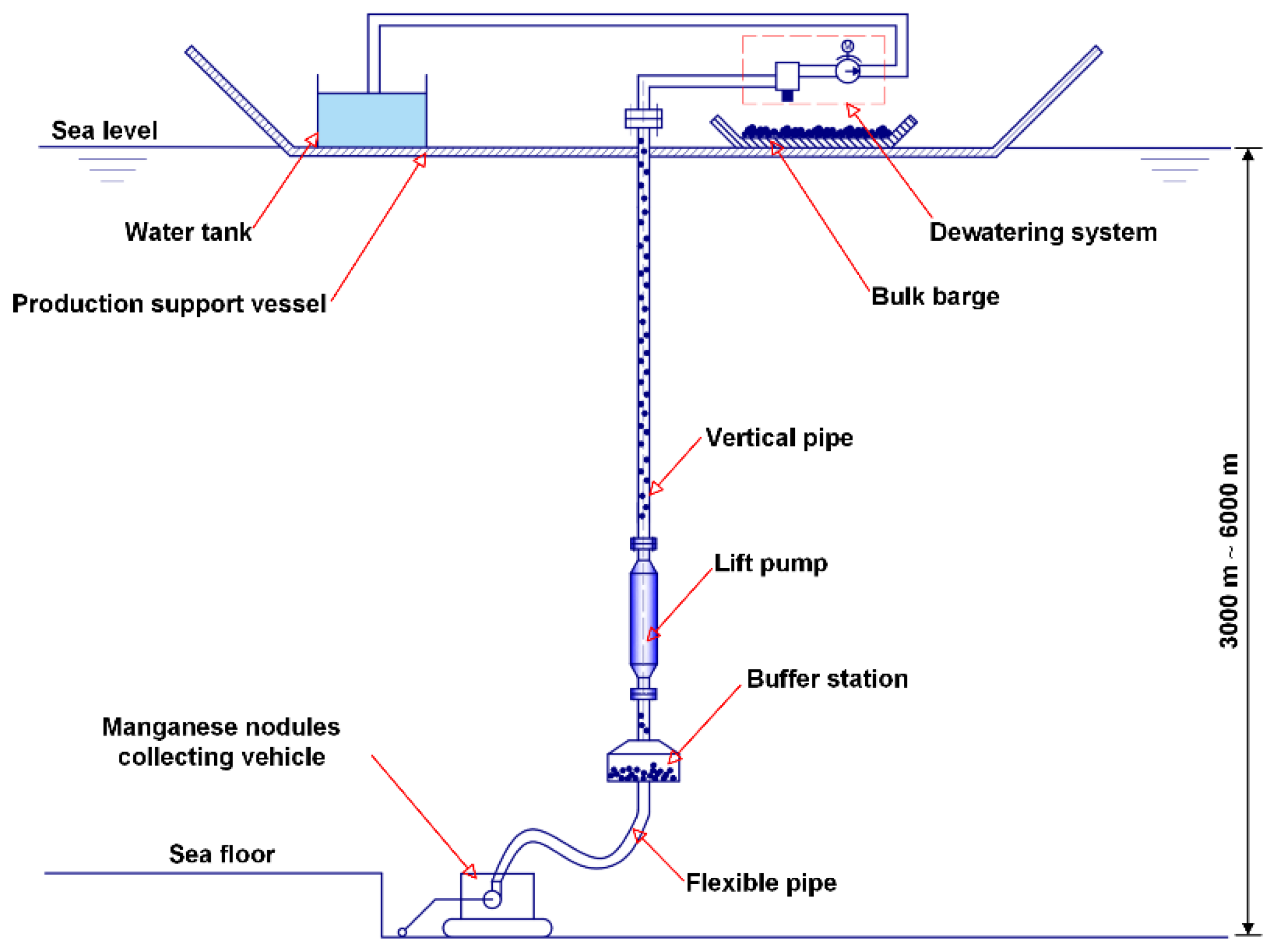
2.1. Geometry Model

Manganese nodules are generally found in the seabed with a depth of 3000 to 6000 m. As shown schematically in Figure 1, the hydraulic mineral lifting system is mainly composed of the mineral collection vehicle, the flexible pipe, the buffer station, the lift pump, the vertical pipe, and the production support vessel. Manganese nodules are collected using the mineral collection vehicle and then pumped via the flexible pipe to the buffer station. The vertical pipe connected to the lift pump is suspended beneath the production support vessel through which the mixture of manganese nodules and seawater is pumped to the sea level. Essentially, the pipe, or pipe segments, covering such a long vertical distance, plays an important role in the lift of manganese nodules. The solid–liquid two-phase flow in the pipe directly affect the stability of the whole system and is influenced by multiple operating parameters such as particle size and solid volume fraction. An unreasonable combination of the operating parameters will incur particle retention and then the increase of local solid concentration. Furthermore, the whole system will be paralyzed due to the blockage of the pipe. Therefore, it is of significance to plumb the flow characteristics in the pipe.

2.2. Flow Parameters

The initial mixture velocity, V_mix,0, represents the velocity of seawater and manganese nodules released at the inlet of the pipe and is defined as:

$$V_{\mathit{mix},0}=\frac{Q_l}{A}$$

(1)

where Q_l represents the volume flow rate of seawater at the inlet (m³/s) and A denotes the cross-sectional area of the passage in the pipe (m²).

The initial solid volume fraction, C_v,0, is defined as the ratio of the volume flow rate of solid particles to the volume flow rate of the liquid released at the inlet of the pipe:

$$C_{v,0}=\frac{Q_s}{Q_l}\times 100\%$$

(2)

Due to the velocity gap between solid particles and seawater, local solid volume fraction might be higher than the initial solid volume fraction C_v,0. The definition of local solid volume fraction, C_v,t, is given by:

$$C_{v,t}=\frac{B_{s,t}}{B_{\mathit{pipe}}}\times 100\%$$

(3)

where B_s,t denotes the total volume of manganese nodules in the pipe at time t (m³) and B_pipe is the volume of the pipe (m³).

For a deep-sea mining system, the mechanisms of the total pressure drop as manganese nodules are transported have not been elucidated. Here, the formulae proposed in [10] are used to provide a reference for the numerically obtained results. A non-dimensional total pressure drop in a vertical pipe, I_v, is defined as:

$$I_v=\frac{\mathsf{\Delta }P}{{\rho }_l\mathit{gL}}$$

(4)

where ΔP denotes the pressure difference between the inlet and outlet of the vertical pipe (Pa), ρ_l denotes the density of liquid (kg/m³), g denotes the acceleration of gravity (m/s²), and L denotes the pipe length (m).

The total pressure drop in the pipe is composed of three parts:

$$I_v=I_l+I_s+I_c$$

(5)

where I_l represents the pressure drop due to the friction between liquid and wall, I_s denotes the pressure drop due to the presence of solid particles, and I_c is related to particle–particle and particle–wall collisions.

I_l is given by:

$$I_l={\lambda }_l\frac{V_{\mathit{mix},0}^2}{2\mathit{gD}}$$

(6)

where V_mix,0 denotes the initial mixture velocity (m/s), λ_l = 0.11(Δ/D + 68/Re)^0.25 is the friction coefficient, and Δ/D is the pipe-wall relative roughness.

I_s is given by:

$$I_s=C_{v,t}\left(\frac{{\rho }_s}{{\rho }_l}-1\right)$$

(7)

where ρ_s is the density of solid particles (kg/m³).

The average liquid velocity V_l (m/s) at the radial position r (m) is obtained by averaging the axial velocity magnitudes of the liquid V_l,i (m/s, in vertical direction) in the region [r − 0.05r, r + 0.05r] of the pipe.

$$V_l\left(r\right)=\frac{1}{n}{\displaystyle \sum }_{i=1}^n{V}_{l,i}\in [r-0.05r, r+0.05r]$$

(8)

Based on Equation (8), the average solid velocity vs. (m/s) and average slip velocity V_slip (m/s) can be attained. The radial position r denotes the distance between the axis of the pipe and the center of the particle, so there is an excluded region for large r. It should be noted that the slip velocity is the difference between the velocities of liquid and particles at the position where particles exist. The average slip velocity is not equal to V_l − Vs.

The average solid volume fraction (SVF) at the radial position r refers to the ratio of the volume of the solid particles to that of the pipe in the region [r − 0.05r, r + 0.05r].

$$C_{v,ave}(r)=\frac{{\displaystyle \sum }{B}_{s,i}\in [r-0.05r,r+0.05r]}{B_{pipe}\in [r-0.05r,r+0.05r]}\times 100\%=\frac{{\displaystyle \sum }{B}_{s,i}\in [r-0.05r,r+0.05r]}{\pi \left\{{(r+0.05r)}^2-{(r-0.05r)}^2\right\}L}\times 100\%$$

(9)

3. Mathematical Models

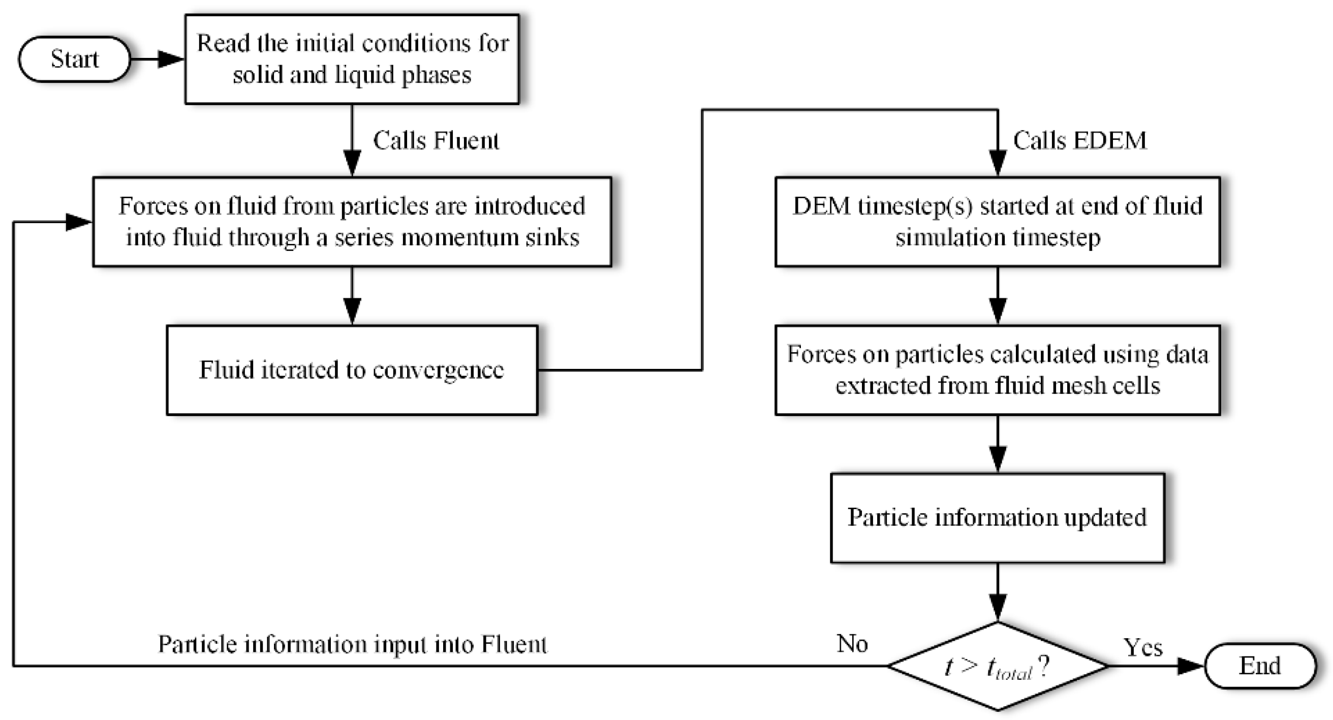
3.1. Computational Model

A two-way coupling method for the solid–liquid two-phase flow was established based on the Euler-Lagrange model. The commercial software ANSYS Fluent 18.0 was used to solve the flow field based on the Euler coordinate system. Meanwhile, the commercial software EDEM 2018 was used to describe the motion of solid particles in the Lagrange coordinate system. ANSYS Fluent and EDEM are connected using compile UDF (User Defined Function, which can be loaded into ANSYS Fluent to control the coupling between ANSYS Fluent and EDEM). Figure 2 shows the flow chart of the coupling between EDEM and Fluent to describe the simulation process. In ANSYS Fluent, for each time step, after convergence was accomplished, the flow data was conveyed to EDEM. Then iterations were performed in EDEM at the same time step to calculate the interaction forces based on the parameters of fluid and solid particles in the same computational element. Subsequently, the information of solid particles was updated and transmitted to ANSYS Fluent. The above steps were repeated until the total simulation time t_total was accomplished [19].

For the flow simulation in the coupling process, the Euler model is used to calculate flow parameters. The effect of the solid phase is considered through introducing the volume fraction of the liquid phase, ε_l.

The continuity equation of the liquid phase is expressed as:

$$\frac{\partial \left({\epsilon }_l{\rho }_l\right)}{\partial t}+\nabla ·\left({\epsilon }_l{\rho }_l{\mathit{u}}_l\right)=0$$

(10)

The momentum equation of the liquid phase is given by [20]:

$$\frac{\partial \left({\epsilon }_l{\rho }_l{\mathit{u}}_l\right)}{\partial t}+\nabla ·\left({\epsilon }_l{\rho }_l{\mathit{u}}_l{\mathit{u}}_l\right)=-{\epsilon }_l\nabla \mathit{P}+\nabla ·\left({\epsilon }_l{\mu }_l\nabla {\mathit{u}}_l\right)+{\epsilon }_l{\rho }_l\mathit{g}+{\mathit{F}}_{sl}$$

(11)

$${\mathit{F}}_{sl}=-\frac{{\displaystyle \sum }{\mathit{F}}_{l_{s,i}}}{\mathsf{\Delta }{V}_{cell}}$$

(12)

where t denotes time (s), u_l denotes the velocity of the liquid phase (m/s), P denotes the static pressure of the liquid phase (Pa), μ_l denotes the dynamic viscosity of the liquid phase (Pa·s), g denotes the acceleration of gravity (m/s²), F_sl denotes the sum of the forces acting on the liquid phase by solid particles in the computational cell (N), F_ls,i denotes the force acting on particle i by the liquid phase (N), and ∆V_cell denotes the volume of the cell (m³).

For the EDEM part, the Lagrange model is used to track the trajectories of solid particles. The translation and rotation of solid particles are governed by Newton′s equation, which is expressed as [21]:

$$m_i\frac{d{v}_i}{dt}={\displaystyle \sum }_j{\mathit{F}}_{c,ij}+{\displaystyle \sum }_k{\mathit{F}}_{nc,ik}+{\mathit{F}}_{ls,i}+{\mathit{F}}_{g,i}$$

(13)

$${\mathit{I}}_i\frac{d{\mathit{\omega }}_i}{dt}={\displaystyle \sum }_j\left({\mathit{M}}_{t,ij}+{\mathit{M}}_{r,ij}\right)$$

(14)

where m_i denotes the mass of solid particle i (kg), v_i denotes the translational velocity of solid particle i (m/s), F_c,ij denotes the contact forces between particles i and j (N), F_nc,ik denotes the non-contact forces between particles i and k (N, e.g., electromagnetic force), F_ls,i denotes the force acting on particle i by the liquid phase (N, e.g., pressure gradient force, drag force, etc.), F_g,i denotes the volumetric force acting on particle i (N, e.g., gravity), I_i denotes the inertia moment of particle i (N·m), ω_i denotes the angular velocity of particle i (rad/s), M_t,ij denotes the tangential friction moment between particles i and j (N·m), and M_r,ij denotes the normal friction moment between particles i and j (N·m).

3.2. Particle Collision Model

It is of significance to establish the model that describes the contact between particles. The contact force, F_c,ij, including the elastic force and the dissipation force, is composed of the normal stiffness force, the normal damping force, the tangential stiffness force, and the tangential damping force:

$${\mathit{F}}_{c,ij}={\mathit{F}}_{cn,ij}+{\mathit{F}}_{ct,ij}={\mathit{F}}_{cn,ij}^s+{\mathit{F}}_{cn,ij}^d+{\mathit{F}}_{ct,ij}^s+{\mathit{F}}_{ct,ij}^d$$

(15)

The Hertz–Mindlin contact model features high accuracy and high efficiency and was employed in the present study [22]. The forces in this model are expressed as:

$${\mathit{F}}_{cn,ij}=\frac{4}{3}{E}_{ij}^{\ast }\sqrt{R^{\ast }}{\delta }_n^{\frac{3}{2}}$$

(16)

$${\mathit{F}}_{ct,ij}=-S_{t,ij}{\delta }_{t,ij}$$

(17)

$${\mathit{F}}_{cn,ij}^d=-2\sqrt{\frac{5}{6}}\beta \sqrt{S_{n,ij}{m}_{ij}^{\ast }}{v}_{n,ij}^{rel}$$

(18)

$${\mathit{F}}_{ct,ij}^d=-2\sqrt{\frac{5}{6}}\beta \sqrt{S_{t,ij}{m}_{ij}^{\ast }}{v}_{t,ij}^{rel}$$

(19)

Taking rolling friction into consideration by applying a torque onto the contacting surfaces yields:

$${\mathit{\tau }}_i=-{\mu }_r{F}_n{R}_i{\mathit{\omega }}_i$$

(20)

where E^* is the equivalent Young’s modulus (Pa), R^* is the equivalent radius (m), δ_n represents the normal overlap (m³), m^* is the equivalent mass (kg), β is the coefficient of restitution, S_n is the normal stiffness (N/m²), $v_{n,\mathit{ij}}^{\mathit{rel}}$ is the normal component of the relative velocity (m/s), S_t is the tangential stiffness (N/m²), δ_t denotes the tangential overlap (m³), $v_{t,\mathit{ij}}^{\mathit{rel}}$ is the relative tangential velocity (m/s), μ_r is the coefficient of rolling friction, F_n is the normal force (N), R_i is the distance of the contact point from the center of mass (m), and ω_i is the angular velocity of particle i at the contact point (rad/s).

3.3. Particle–Wall Collision Model

For the particle–wall model, the equations are almost the same as the particle collisions. Only the calculation methods of equivalent radius and mass between wall and particle need to be changed. Supposing the radius and mass of the wall are $R_{\mathit{wall}}=\infty$ and $m_{\mathit{wall}}=\infty$, the equivalent radius and mass can be obtained as $R_{i,\mathit{wall}}^{*}=R_i$ and $m_{i,\mathit{wall}}^{*}=m_i$.

3.4. Forces Acting on Particles by Seawater

In the horizontal direction, the particle is mainly affected by Magnus lift force, F_M, Saffman lift force, F_S, and turbulence force, F_t. Magnus lift force and Saffman lift force, pointing to the center of the pipe, are caused by the velocity difference between two sides of the particle. Turbulent force originates from the fluctuation of the liquid flow parameters. In the vertical direction, the particle suffers from gravitational force, F_g, pressure gradient force, F_p, and drag force, F_D. The gravitational force is opposite to the flow direction while the directions of pressure gradient force and drag force are consistent with the flow direction [23,24,25,26].

When a particle rotates in the flow field, a force perpendicular to the relative velocity of the particle will be produced, which is termed Magnus lift force.

$${\mathit{F}}_M=\frac{1}{8}\pi d_s^3{\rho }_l{\mathit{\omega }}_i\times \left({\mathit{u}}_l-{\mathit{u}}_s\right)$$

(21)

where u_s is the velocity of particle (m/s) and d_s is the diameter of particle i (m).

When a particle moves in the flow field with high velocity gradients, the particle undergoes the force from high pressure to low pressure, which is termed Saffman lift force.

$${\mathit{F}}_S=1.61d_s^2\left({\mathit{u}}_l-{\mathit{u}}_s\right)\sqrt{{\rho }_l{\mu }_l}{\left|\frac{d{\mathit{u}}_l}{dy}\right|}^{1/2}$$

(22)

where μ_l is the dynamic viscosity of the liquid (Pa·s).

Gravity is the force produced by the earth and is given by:

$${\mathit{F}}_g=\frac{1}{6}\pi d_s^3{\rho }_s$$

(23)

When a particle moves in the flow field with pressure gradients, it will be subjected to the pressure gradient force:

$${\mathit{F}}_p=-\frac{1}{6}\pi d_s^3\nabla \mathit{P}$$

(24)

Due to the velocity gap between particles and liquid, the particles suffer from the drag force affected by the particle Reynolds number Re_p, the turbulent parameters, and the shape and concentration of particles, and so on.

$${\mathit{F}}_D=C_D\frac{{\rho }_l\left|{\mathit{u}}_l-{\mathit{u}}_s\right|\left({\mathit{u}}_l-{\mathit{u}}_s\right)}{2}\frac{\pi d_s^2}{4}$$

(25)

where C_D is the drag coefficient, which is set to 0.44 when Re_p > 1000.

4. Numerical Preparations

4.1. Numerical Setup

Duplex stainless steel was selected as the material of the vertical pipe. The pipe has an inner diameter of 0.1 m and a length of 5 m. Manganese nodules, with a density of 2040 kg/m³ served as solid particles. Seawater, with temperature of 24 °C, density of 1044 kg/m³, and dynamic viscosity of 1.01 × 10⁻³ Pa·s, was used as the liquid phase. The reference pressure was set to 101,325 Pa. The outflow boundary condition was defined at the outlet of the computational domain. No-slip boundary conditions were set at all walls wetted by the two-phase flow. The surface roughness of the inner wall of the pipe was set to 100 μm, which is equivalent to the practical situations.

CFD-DEM simulations require appropriate time steps for both solid and liquid phases. The solid time step is limited by Rayleigh time Δt_R, which is given by:

$$\mathsf{\Delta }{t}_R=\pi \frac{d_s}{2}{\left(\frac{{\rho }_s}{G_s}\right)}^{\frac{1}{2}}{\left(0.1631{\sigma }_s+0.8766\right)}^{-1}$$

(26)

where d_s is the diameter of the particle (m), ρ_s is the density of the particle (kg/m³), G_s is the shear modulus of the particle (Pa), and σ_s is the Possion’s ratio of the particle. According to the particle properties used in the study, the Δt_R is calculated as about 1.6×10⁻⁴ s. The DEM time step Δt_s is often smaller than the Rayleigh time and is set to 1.0 × 10⁻⁴ s. The CFD time step Δt_l is set to 1.0 × 10⁻³ s, which should be 10~100 times the DEM time step. The total simulation time is 3 s, in which the residual converges below 10⁻³ in Fluent. The parameter settings of EDEM and ANSYS Fluent are listed in

Table 1. Parameter settings for EDEM and ANSYS Fluent [27].

Pipe parameters
Diameter (m)	0.1
Length (m)	5
Poisson’s ratio	0.3
Density (kg/m3)	7980
Shear modulus (Pa)	7.0 × 107
Particle–wall restitution coefficient	0.52
Particle–wall static friction coefficient	0.16
Particle–wall rolling friction coefficient	0.01
Liquid property
Liquid density (kg/m3)	1044
Liquid temperature (°C)	24
Liquid viscosity (Pa·s)	1.01 × 10−3
Solid particle property
Poisson’s ratio	0.4
Density (kg/m3)	2040
Shear modulus (Pa)	2.13 × 107
Particle–particle restitution coefficient	0.45
Particle–particle static friction coefficient	0.28
Particle–particle rolling friction coefficient	0.01
CFD reference pressure (Pa)	101,325
CFD time step (s)	0.001
CFD turbulence model	RNG k-ε
DEM time step (s)	0.0001
Total simulation time (s)	3

.

Table 2. Operating conditions for present simulations.

Operating Parameters	No.	Initial SVF, Cv,0 (%)	Particle Diameter, ds (mm)	Initial Mixture Velocity, Vmix,0 (m/s)
Effects of Cv,0	Case 1	1	15	4
	Case 2	5	15	4
	Case 3	10	15	4
Effects of Vmix,0	Case 4	5	15	3
	Case 5	5	15	4
	Case 6	5	15	4.5
Effects of ds	Case 7	5	5	4
	Case 8	5	15	4
	Case 9	5	30	4

summarizes the cases simulated. The initial SVF (C_v,0) indicates the ratio of the volume flow rate of particles to that of liquid at the inlet of the vertical pipe. The values of initial SVF were set to 1%, 5%, and 10%. The shape of the particles was defined as spherical. Three particle diameters, 5.0 mm, 15.0 mm, and 30.0 mm, were selected. The initial mixture velocity represents the velocity of the liquid and solid released at the inlet of the pipe, and it varies between 3 m/s, 4 m/s, and 4.5 m/s. The direction of the initial mixture velocity is comparable to the inlet section of the pipe.

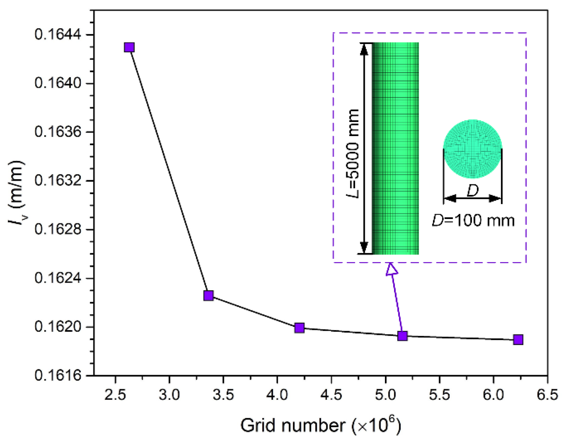
4.2. Grid Generation

The vertical pipe, with an inner diameter of 100 mm and a length of 5000 mm, was used for numerical simulation. The flow domain in the pipe was discretized by structured grids. A grid-independence examination was performed, and five grid schemes were devised. The same numerical setting was applied for the five grid schemes, and the total pressure drop was monitored. According to the obtained results, as the total grid number increases, I_v decreases continuously, as shown in Figure 3. Furthermore, as the total grid number exceeds 5 million, the relative difference of I_v between neighboring grid schemes is less than 5%. In consideration of both numerical accuracy and economy, the grid scheme with the total grid number of 5,115,844 was selected in subsequent simulations.

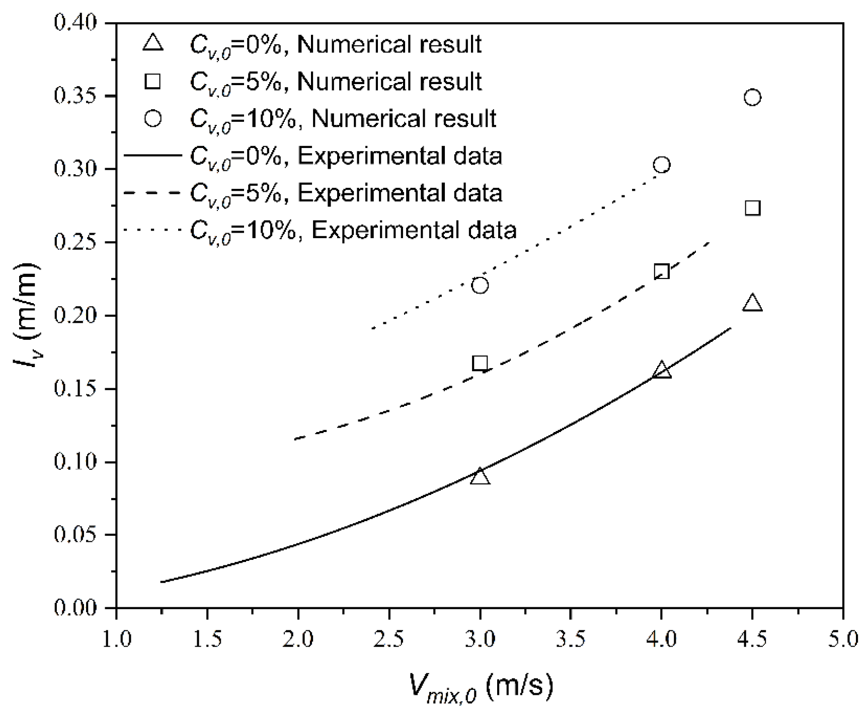
4.3. Experimental Validation

The numerically obtained total pressure drop of the flow with particles of d_s = 15.0 mm was compared with the experimental result to examine the validity of the numerical scheme. More details regarding the experimental work can be found in [5]. The relationship between the total pressure drop and the initial mixture velocity in the vertical pipe is illustrated in Figure 4. It is evidenced that the numerical results agree well with the experimental data. As the initial mixture velocity increases, the total pressure drop increases, which is insensitive to the initial SVF. Furthermore, a high initial SVF is associated with a high total pressure drop. The maximum deviation between the numerical and experimental results is less than 5%, which proves high physical validity of the numerical scheme.

5. Results and Discussion

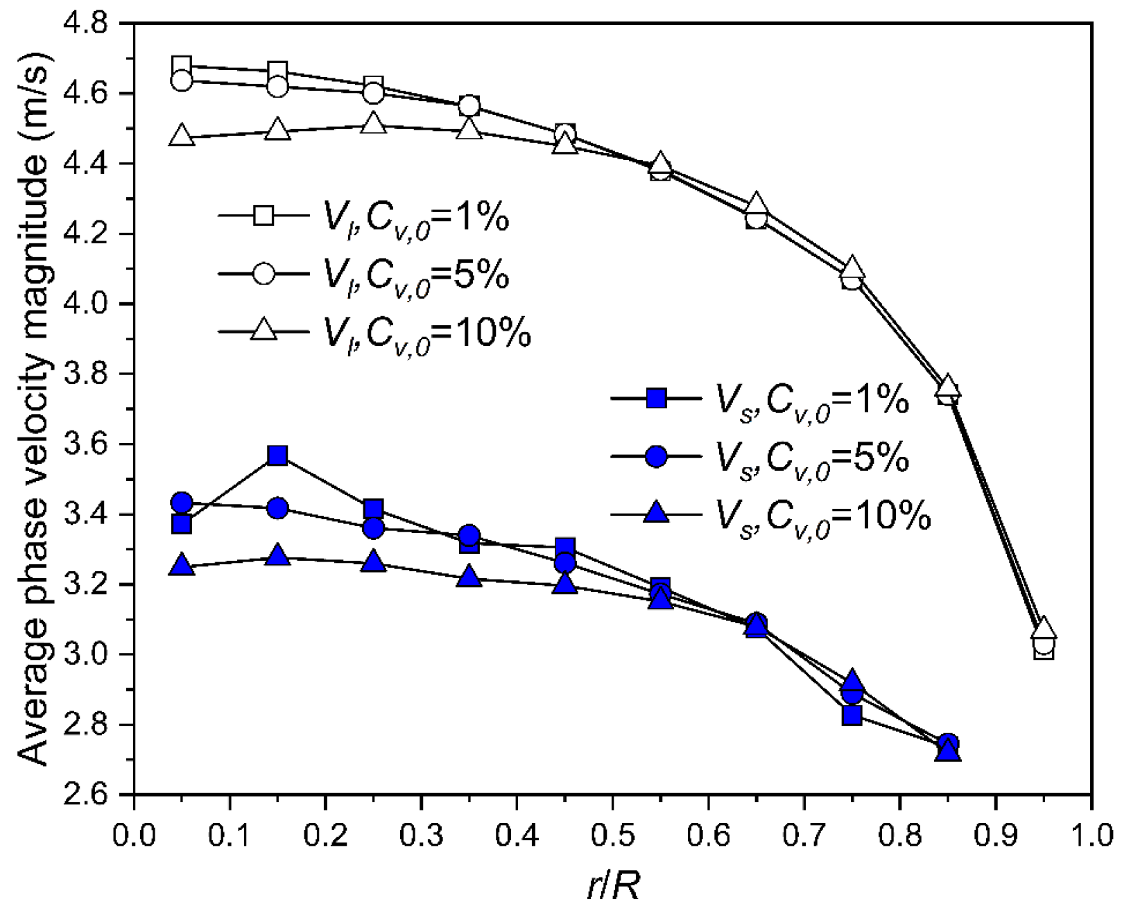
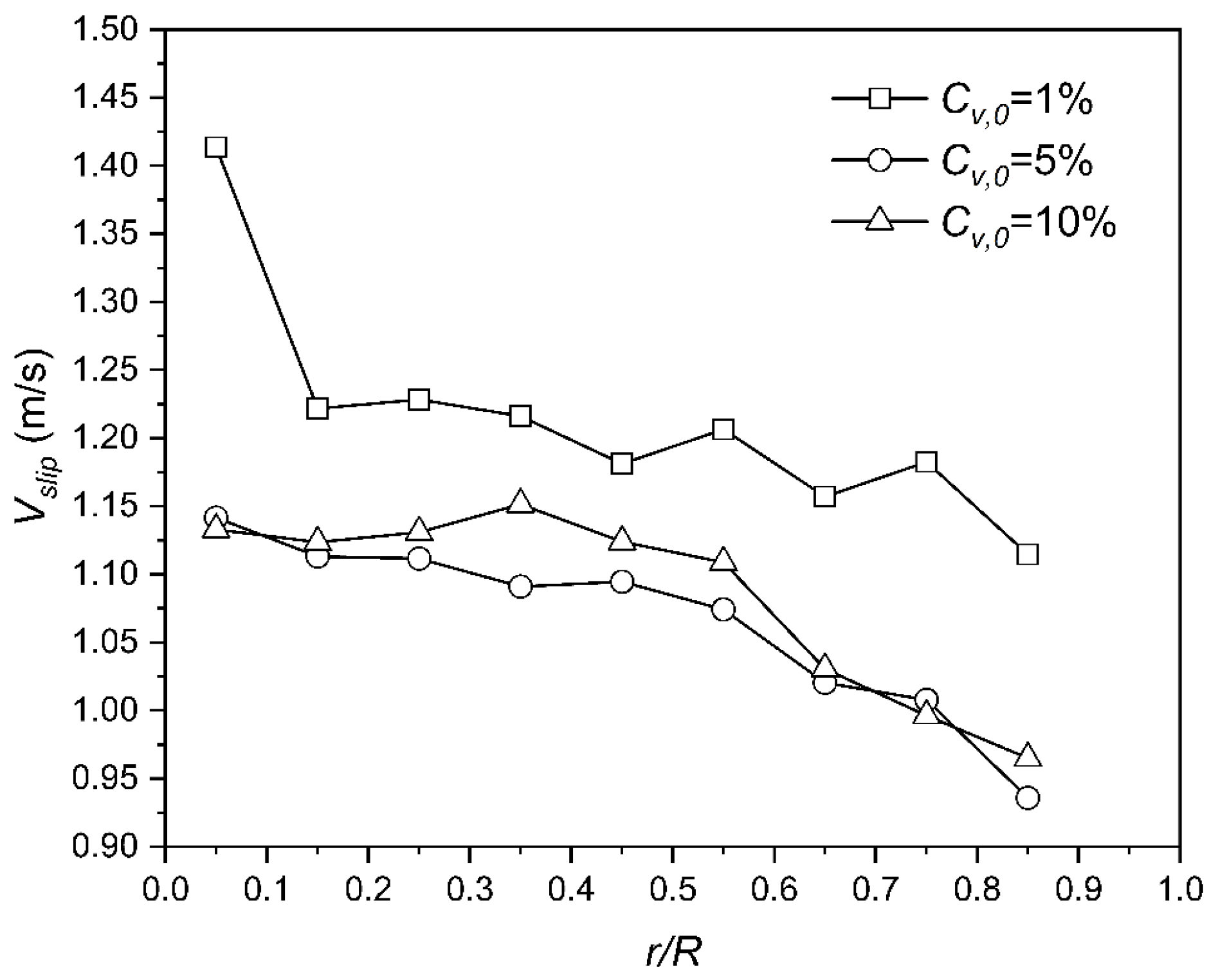
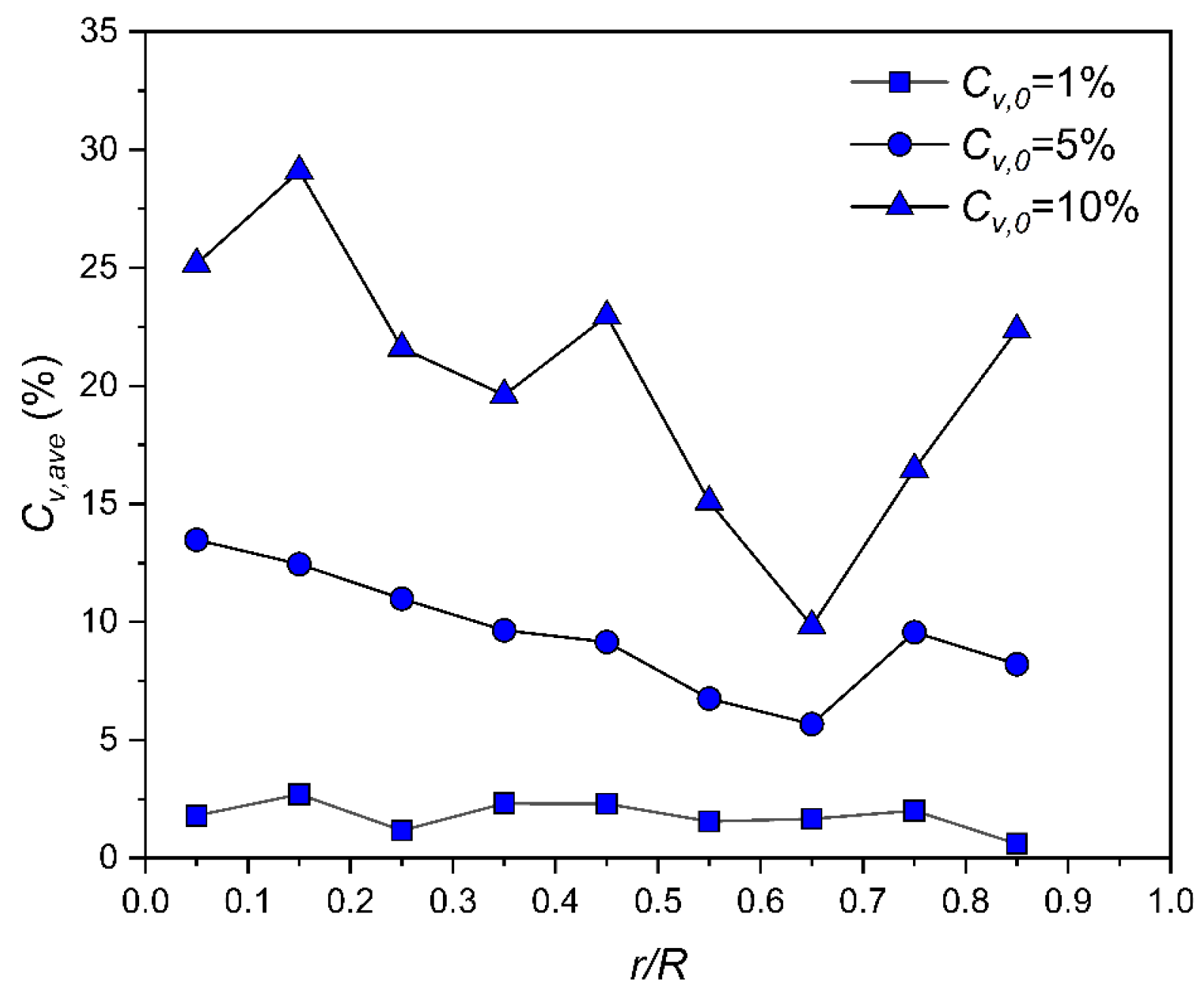
5.1. Effect of Initial Solid Volume Fraction

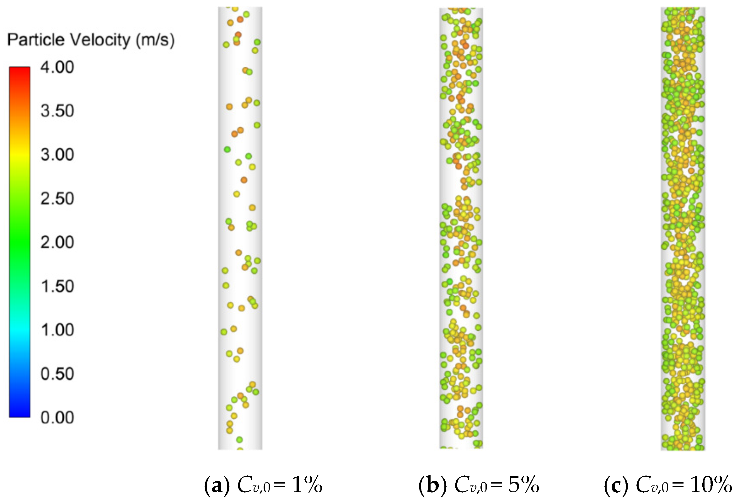
5.1.1. Distribution of Instantaneous Particle Velocity

At V_mix,0 = 4.0 m/s and d_s = 15.0 mm, instantaneous particle velocity distributions at different initial SVFs are shown in Figure 5. It is interesting that particles with high velocities tend to concentrate in the central zone of the pipe, while low-velocity particles gather near the wall, which is consistent with the results obtained in [28]. Essentially, liquid velocity in the central zone is higher than that near the wall due to the effect of friction between the liquid and the wall. Furthermore, particles tend to move towards the pipe axis, minimizing the energy loss induced by particle–wall interactions.

At low initial SVF, as shown in Figure 5a, the particles are dispersed over the cross-section. Such a pattern has only been observed at the initial SVFs higher than 5% and for small particles with diameters less than 2.3 mm [3]. This particle scattering phenomenon becomes more remarkable with increasing initial SVF. The particles separate from each other due to collision. As the initial SVF increases, the collision between particles is intensified. It is demonstrated in Figure 5 that the particle velocity decreases with increasing initial SVF, which is more evident in Figure 6. The pressure energy serves as a source for the kinetic energy of liquid and particles. With more particles delivered, the sum of the kinetic energy of particles increases, resulting in a high total pressure drop. However, if the sum of the kinetic energy of particles is averaged over all particles, each particle shares less kinetic energy than that associated with small particle number. Therefore, particle velocity decreases with increasing particle number, as shown in Figure 6. Meanwhile, inevitable energy loss during the transport process is caused by friction and collisions. Furthermore, with increasing initial SVF, the reinforced contacts between particles and between particles and the wall incur energy loss. Moreover, collisions between particles are intensified as particle number increases, which intensifies energy consumption and increases in total pressure drop.

5.1.2. Average Parameters

At V_mix,0 = 4.0 m/s and d_s =15.0 mm, the average rising velocity of seawater is plotted as a function of non-dimensional radial position in Figure 6. With increasing initial SVF, the average seawater velocity decreases from about 4.7 m/s to 4.5 m/s in the central zone, but the variation of the average seawater velocity with initial SVF is negligible near the wall. This trend agrees well with the experimental observation [29]. At a given particle size, the increase in initial SVF leads to the participation of more particles. Consequently, more energy will be consumed and both seawater and particle velocities decrease as initial SVF increases, as indicated in Figure 6. In the central zone and as initial SVF increases from 5% to 10%, the seawater velocity decreases by about 0.7 m/s while the velocity of manganese nodules decreases by about 0.5 m/s. Due to the effect of wall shear, the seawater velocity decreases remarkably near the wall, while manganese nodules suffer less from this effect. In addition, seawater in the central zone accelerates much easier than manganese nodules due to considerably lower density. There is a jump in the value of average solid velocity for C_v,0 = 1% between r/R = 0.05 and r/R = 0.15. Compared with C_v,0 = 5% and 10%, the number of particles at the center of the pipe is not dominant for C_v,0 = 1%. The smaller the particle number, the higher the slip velocity needed to create the drag force to balance the gravity and the buoyancy force in a vertical direction. Therefore, average solid velocity is low at the pipe center.

The average slip velocities for different initial SVFs are plotted as a function of r/R in Figure 7. It can be seen that the average slip velocity decreases generally with increasing radial distance from the pipe axis. It is also evidenced that the slip velocities for C_v,0 = 5% and 10% decrease remarkably compared to that corresponding to C_v,0 = 1%. For particles with diameters of 5.0 mm, 15.0 mm, and 30.0 mm, the settling velocities are about 0.353 m/s, 0.612 m/s, and 0.865 m/s, respectively, which were calculated through $u_t=\sqrt{\frac{8}{3}{d}_{s}g\frac{\left({\rho }_s-{\rho }_l\right)}{{\rho }_l}}$. For a particle falling or rising in both static and dynamic fluid, it mainly suffers from the drag force, the buoyancy force, and the gravity force in a vertical direction. As the liquid velocity increases, the drag coefficient of particle is reduced. The drag force is related to the drag coefficient and the slip velocity. After the balance of forces is attained, the slip velocities of the three cases are all greater than their settling velocities.

The distribution of average solid volume fraction C_v,ave in a radial direction is shown in Figure 8, where r is the distance between the center of the particle and the cross-sectional center of the pipe and R denotes the radius of the pipe. It is evidenced that the average SVF decreases with radial position r generally. Furthermore, the reduction of initial SVF promotes the uniformity of the distribution of manganese nodules. The lift force and the pressure gradient force have insignificant influence on the lateral movement of particles, which is ascribed to the low rotation intensity of particles and uniform pressure gradients over the cross section. Therefore, the contact force plays an important role in determining the particle distribution along the radial direction. At high initial SVFs, some particles at the cross-sectional center are exposed to contact forces from all directions because they are surrounded by other particles. However, the contact forces counteract each other; consequently, central particles can move stably with large average SVF, and lateral movement is not influential. Surrounding particles will be bounced back towards the wall after they interact with the central particles. Therefore, the average SVF increases sharply near the wall with the initial SVF. In comparison, at low initial SVFs, particles exhibit a relatively random pattern of motion because the contact forces cannot be effectively counteracted. Therefore, low initial SVF results in a more uniform distribution of particles.

5.1.3. Total Pressure Drop

The variation of the total pressure drop with initial SVF is listed in

Table 3. Relationship between total pressure drop and initial SVF at V_mix,0 = 4.0 m/s and d_s = 15.0 mm.

Cv,0 (%)	1	5	10
Cv,t (%)	1.3	6.8	14.8
Iv (m/m)	0.1753	0.2303	0.3127

. The total pressure drop, I_v, is composed of three parts, as illustrated in Equation (5). I_s is related to the local SVF and the density of manganese nodules. I_l depends on the seawater velocity, which influences the friction loss between seawater and the pipe wall [30]. For a given particle size and the initial mixture velocity, the total pressure drop increases with initial SVF, which can be reasonably explained by the energy balance during the transport process. Liquid and particles derive their kinetic and potential energy mainly from the pressure drop through the pipe. As the initial SVF increases, the sum of the kinetic or potential energy of particles increases. Moreover, increased frequencies of collisions cause more energy loss of the two-phase flow. Therefore, high initial SVFs are responsible for the low pressure energy of the liquid at the outlet and a corresponding high pressure drop due to the enlarging of the difference of pressure energy between inlet and outlet. It is noteworthy that, in CFD code, relative pressure in the fluid domain is adopted so that the outlet pressure may be less than 0 Pa. However, in practical applications, the gauge pressure at the outlet of the pipe should be larger than 0 Pa, so fluid machinery is required to provide additional energy for conveying the mixture to prevent reverse flow. According to Equations (6) and (7), it seems that hydraulic transport with a higher SVF is more economical. However, increasing the initial SVF can cause a decrease of particle velocity. When particle velocities are lower than three times the settling velocity, this may incur retention and even blockage. Therefore, the selection of appropriate parameters, such as the initial SVF, the initial mixture velocity, and particle diameter, is vital for the transport of the mixture.

5.2. Effect of Particle Diameter

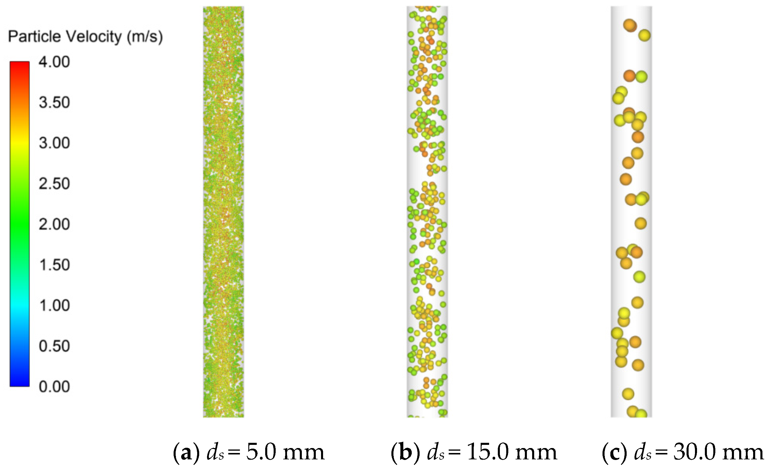
5.2.1. Distribution of Instantaneous Particle Velocity

At V_mix,0 = 4.0 m/s and C_v,0 = 5%, characteristic particle velocity distributions at different particle diameters are shown in Figure 9. It is evidenced that the local SVF decreases significantly, and the distribution range of particles is apparently narrowed as particle diameter increases. At certain initial SVF, the number of large particles is smaller than that of small particles. Meanwhile, the flow velocity with large particles involved is higher than that associated with small particle. This implies that the volume of the mixture transported out of the pipe at a given timespan is larger for large particles.

5.2.2. Average Parameters

As seen in Figure 10, the average liquid velocity attains its maximum at the pipe axis, as is common for the three cases. Particle diameter has a non-negligible effect on the seawater velocity. At d_s = 5.0 mm, the particle number is large, and the energy loss is high owing to frequent interactions between particles and wall. Therefore, the overall flow velocity is lower than the other two cases. However, this tendency is overturned near the wall. Essentially, the frictional loss between the two-phase flow and inner wall of the pipe is alleviated as small particles are transported. Meanwhile, as shown in Figure 10, the particle velocity at d_s = 5.0 mm is low in the central zone but is high near the wall compared to those corresponding to d_s = 15.0 mm and 30.0 mm.

Due to interactions between particles and between particles and the pipe wall, the distributions of the slip velocity in radial directions are not uniform, which is implied in Figure 11. However, a general trend indicates that the slip velocity decreases with the increase of the radial distance from the pipe axis. The slip velocity for d_s = 5.0 mm decreases sharply near the wall. Overall, the slip velocity decreases as particle diameter increases from 15.0 mm to 30.0 mm, which is in accordance with the conclusion reported in [5].

The variation of average SVF differs for the three cases with increasing radial position r/R, as evidenced in Figure 12. For particles with a diameter of 5.0 mm, the average SVF distributes uniformly and only declines near the wall. For particles with a diameter of 15.0 mm, the average SVF increases with the radial position and rises near the wall. The distribution of average SVF for particles of 30.0 mm is similar to that for particles of 5.0 mm at the region far away from the wall. It implies that both high local SVF and low local SVF contribute to the uniform distribution of average SVF except in the region near the wall. At the same initial SVF, the average SVF of small particles is far larger than that of large particles, which implies more energy will be lost due to collisions between particles and the wall.

5.2.3. Total Pressure Drop

The relationship between the total pressure drop and particle diameter is shown in

Table 4. Relationship between total pressure drop and particle diameter at V_mix,0 = 4.0 m/s and C_v,0 = 5%.

ds (mm)	5.0	15.0	30.0
Cv,t (%)	7.0	6.8	6.6
Iv (m/m)	2.3730	0.2303	0.0986

. As the particle diameter increases from 5.0 mm to 15.0 mm, I_v decreases considerably. However, as the particle diameter increases from 15.0 mm to 30.0 mm, I_v varies insignificantly. Relative to the situations at d_s = 15.0 mm and 30.0 mm, the case at d_s = 5.0 mm is more sensitive to the variation of particle diameter. With increasing particle diameter, the number of particles reduces so that I_v decreases due to relieved particle–particle and particle–wall interactions. Furthermore, as small manganese nodules are transported, high local SVF also induces high total pressure drop.

5.3. Effect of Initial Mixture Velocity

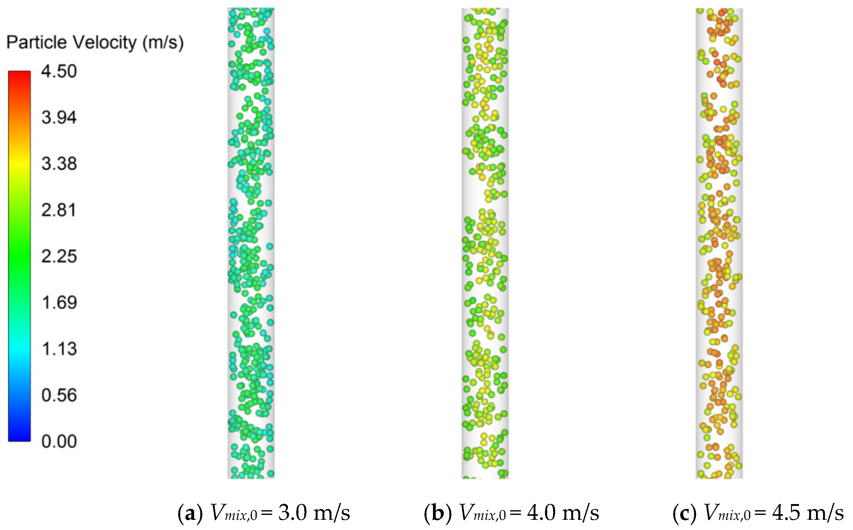
5.3.1. Distribution of Instantaneous Particle Velocity

The distributions of particle velocity at different initial mixture velocities are shown in Figure 13. For a given particle diameter and initial SVF, local SVF decreases as the initial mixture velocity increases, which is related to the decrease in the slip velocity. This implies that the increases of the initial mixture velocity can improve the transport performance of the hydraulic lifting system. At high initial mixture velocities, it is demonstrated that the particles with high velocities accumulate in the central zone of the pipe while low-velocity particles tend to gather near the pipe wall.

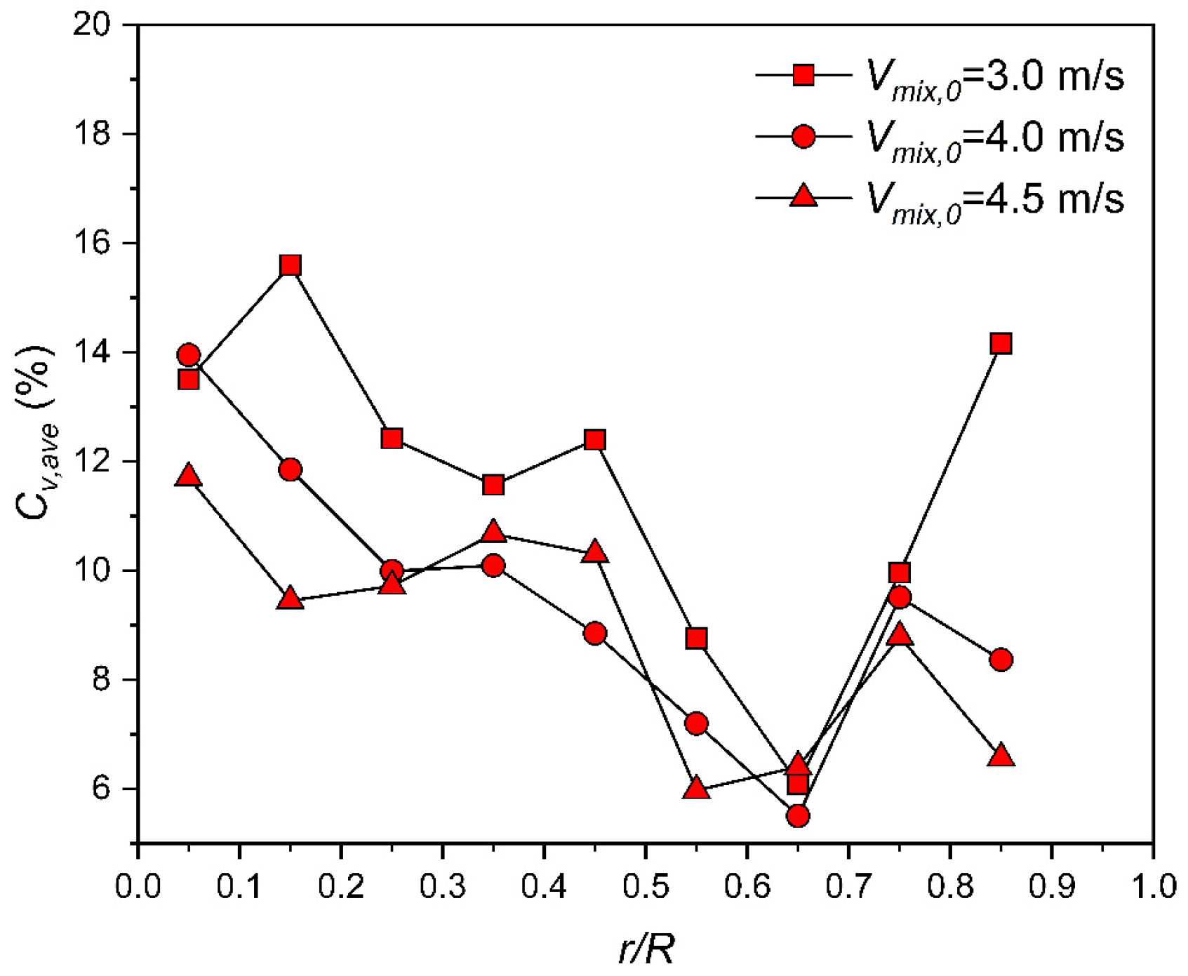
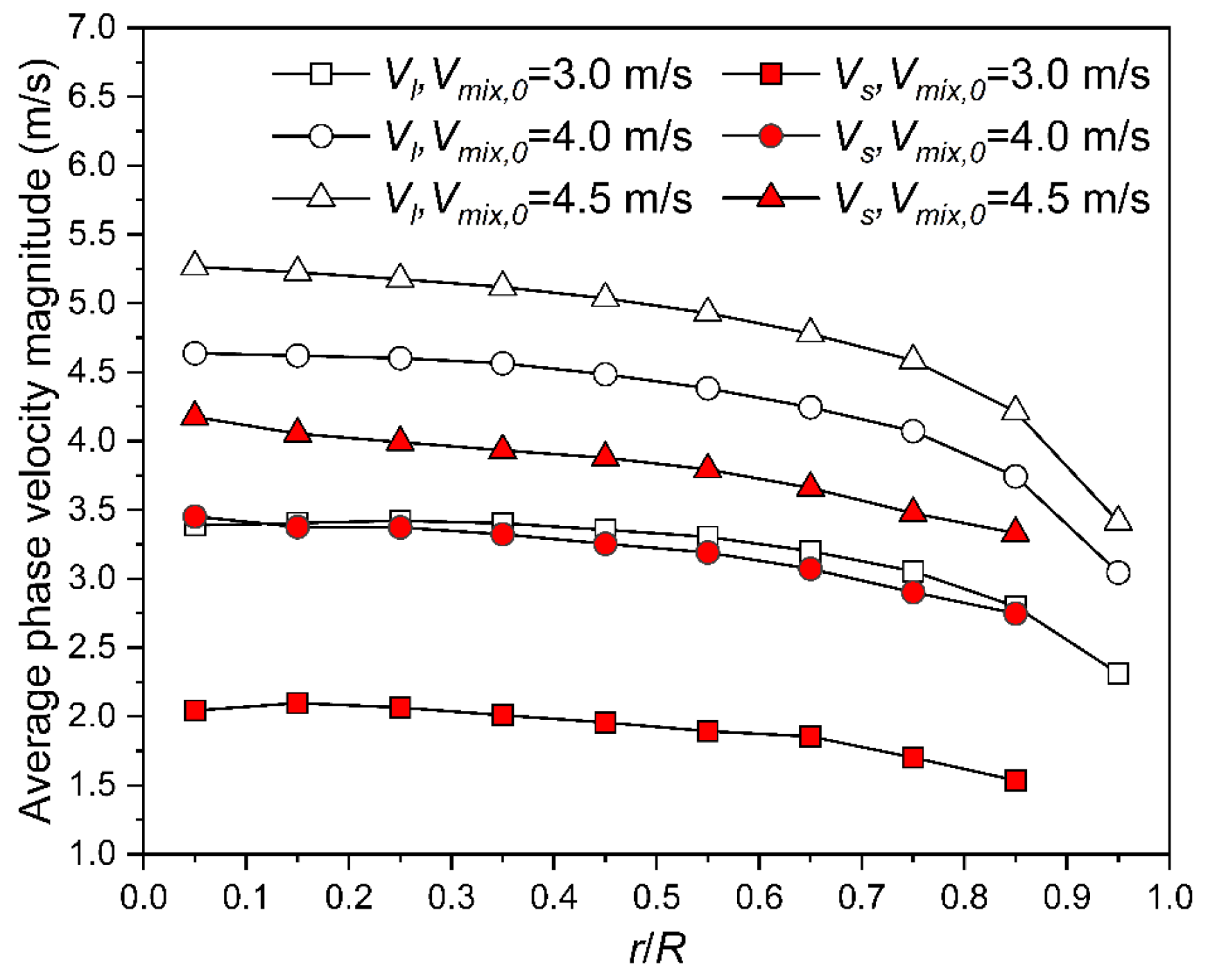
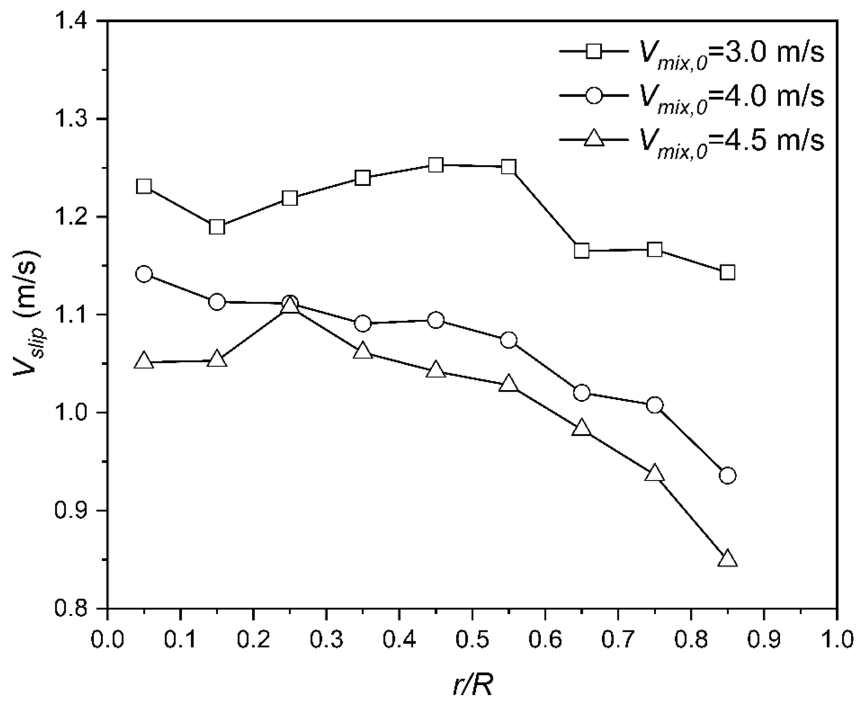
5.3.2. Average Parameters

As seen in Figure 14, the cases featured by different initial mixture velocities have similar average seawater velocity distribution patterns. The maxima of the average liquid and solid velocities arise at the pipe axis, while near the pipe wall, the two velocities reach their minimum values, respectively. Due to the effect of the wall shear, the maximum average liquid velocity is even higher than the initial mixture velocity, and the average liquid velocity near the wall decreases sharply to its minimum. Near the wall, a significant influence of the viscous force results in low average liquid velocity. Meanwhile, at the cross-sectional center, the inertia force promotes the increase in the average liquid velocity. In fact, the kinetic behaviors of the particles are less affected by the wall shear effect. This can be attributed to the low frequency of tangential friction between particles and the wall. However, direct collision between a particle and the wall results in a considerable decrease of the kinetic energy of the particle. Consequently, the average solid velocity decreases continuously in the radial position.

It is evidenced in Figure 15 that the average slip velocity decreases with increasing initial mixture velocity. The drag force depends on the drag coefficient and the liquid velocity. With increasing initial mixture velocity, liquid velocity plays a more important role than the drag coefficient, resulting in the rise of the drag force and the decrease of slip velocity. It is inferable that high initial mixture velocity is beneficial to the conveying of large particles. However, more energy input is necessitated.

It is evidenced in Figure 16 that the initial mixture velocity has a slight effect on average SVF distributions in the pipe. The increase of the initial mixture velocity results in a decrease of the average SVF. For the three cases, average SVFs reach their minimum value around r/R = 0.65 and then rise near the wall. This can be attributed to the fact that particles around r/R = 0.65 prefer to be impacted toward the axis or wall of the pipe. With increasing initial mixture velocity, at given initial SVF, the number of particles released at the inlet increases. However, increasing initial mixture velocity improves the mixture conveying performance, manifesting in the decrease of slip velocity and average SVF. This implies that the ratio of the local SVF to the initial SVF is smaller for larger initial mixture velocities.

5.3.3. Total Pressure Drop

As the initial mixture velocity increases, the total pressure drop increases, which is evidenced in

Table 5. Relationship between total pressure drop and initial mixture velocity at C_v,0 = 5% and d_s = 15.0 mm.

Vmix,0 (m/s)	3.0	4.0	4.5
Cv,t (%)	8.6	6.8	6.4
Iv (m/m)	0.1756	0.2303	0.2736

. The increase of local SVF aggravates the particle–particle and particle–wall interactions. Meanwhile, high flow velocity induces the increase of the friction loss between seawater and the wall. Therefore, the total pressure drop increases.

5.4. Retention Ratio

The retention ratio, C_v,t/C_v,0, is defined to describe the variation of local solid-phase concentration with the initial mixture velocity. In Figure 17, cases of different initial SVFs and particle diameters are presented. It is seen that with increasing initial mixture velocity, the retention ratio decreases continuously, which is common for all of the six cases. This can be attributed to the fact that the drag coefficient decreases with increasing mixture velocity, which implies that necessary slip velocity can be easily attained. At a certain particle diameter and the initial mixture velocity, the increase of the initial SVF contributes to the increase of C_v,t/C_v,0. This could be due to the growing importance of particle–particle and particle–wall interaction in energy dissipation. In addition, the liquid and solid velocities decrease, which means that the mass flow rate of the outlet is smaller than that of the inlet. Despite the fact that particle slip velocity decreases as concentration increases, this is insufficient to compensate for the blocking effect caused by the decrease in mixture velocity and the increase in particle collision. It is seen that variations of the retention ratio with the particle diameter at V_mix,0 = 3 m/s and V_mix,0 = 4 m/s are not monotonic. At V_mix,0 = 3 m/s and 4 m/s, the highest retention ratio is reached at d_s = 15.0 mm and C_v,0 = 10%. For particles exposed to this condition, the ability of following the carrying liquid is explicitly low. The slip velocity becomes increasingly relevant as the initial mixture velocity decreases, resulting in the retention ratio of a large particle being greater than that of a small particle. At V_mix,0 = 4.5 m/s, the retention ratio decreases with increasing particle diameter. At V_mix,0 = 4.5 m/s, highly frequent collisions between particles with d_s = 5.0 mm reduce the liquid and solid velocities, leading to increases in local SVF and the retention ratio. As the influence of slip velocity diminishes with increasing initial mixture velocity, the relationship between particle size and retention ratio varies predictably. In the case of infinite initial mixture velocity, slip velocity can be ignored, resulting in a retention ratio close to 1.

5.5. Relationship between Is + Ic and Local SVF

The pressure drop due to the particle–particle and particle–wall collisions cannot be well evaluated. Here, Equation (7) was improved to describe the pressure drop due to the presence of solid particles as well as collisions through introducing a coefficient k.

$$I_s+I_c={\mathit{kC}}_{v,t}\left(\frac{{\rho }_s}{{\rho }_l}-1\right)$$

(27)

The coefficient k represents the collision intensity and varies with particle diameter. At the same local SVF, the particle kinetic energy and the potential energy obtained from the liquid are roughly the same. However, the number of small particles is larger, which means more frequent collisions and intensified energy dissipation. Therefore, more energy is consumed for the transportation of small particles, leading to a higher total pressure drop. In Figure 18, the numerical data are fitted according to Equation (27). By subtracting the I_l determined by Equation (6) from I_v calculated by Equation (4), the numerical data I_s + I_c is produced. The coefficient k of particles of d_s = 5.0 mm is 25 times that of particles of d_s = 15.0 mm, indicating the energy dissipation due to particle collision cannot be neglected for small particles at high SVF. Through combining Equations (6) and (27), the total pressure drop of the hydraulic transportation with solid particles can be well predicted.

Theoretically, k changes from 0 to infinity when the ratio of particle diameter to pipe diameter changes from 1 to 0. This may not be applicable when the particle size is too small or too large. It is validated in Figure 18 that Equation (27) is applicable when the ratio of particle diameter to pipe diameter changes from 0.05 to 0.3. As far as the application scope of Equation (27) is concerned, it needs to be studied further. However, Equation (27) only applies to a flow free of obstructions. This is because the law of inter-particle collision changes with blockage, which may also cause a surge of local pressure.

6. Conclusions

The hydraulic lifting of manganese nodules was numerically investigated using a CFD-DEM coupling method. The effects of solid volume fraction, particle diameter, and flow velocity were discussed. The major conclusions drawn from the present study are as follows:

(1)

With increasing initial solid volume fraction, the energy consumption is enhanced, which leads to the decreases in both seawater and manganese nodule velocities at the central part of the pipe. This effect attenuates near the wall. Moreover, a high initial solid volume fraction results in an increase in total pressure drop.

(2)

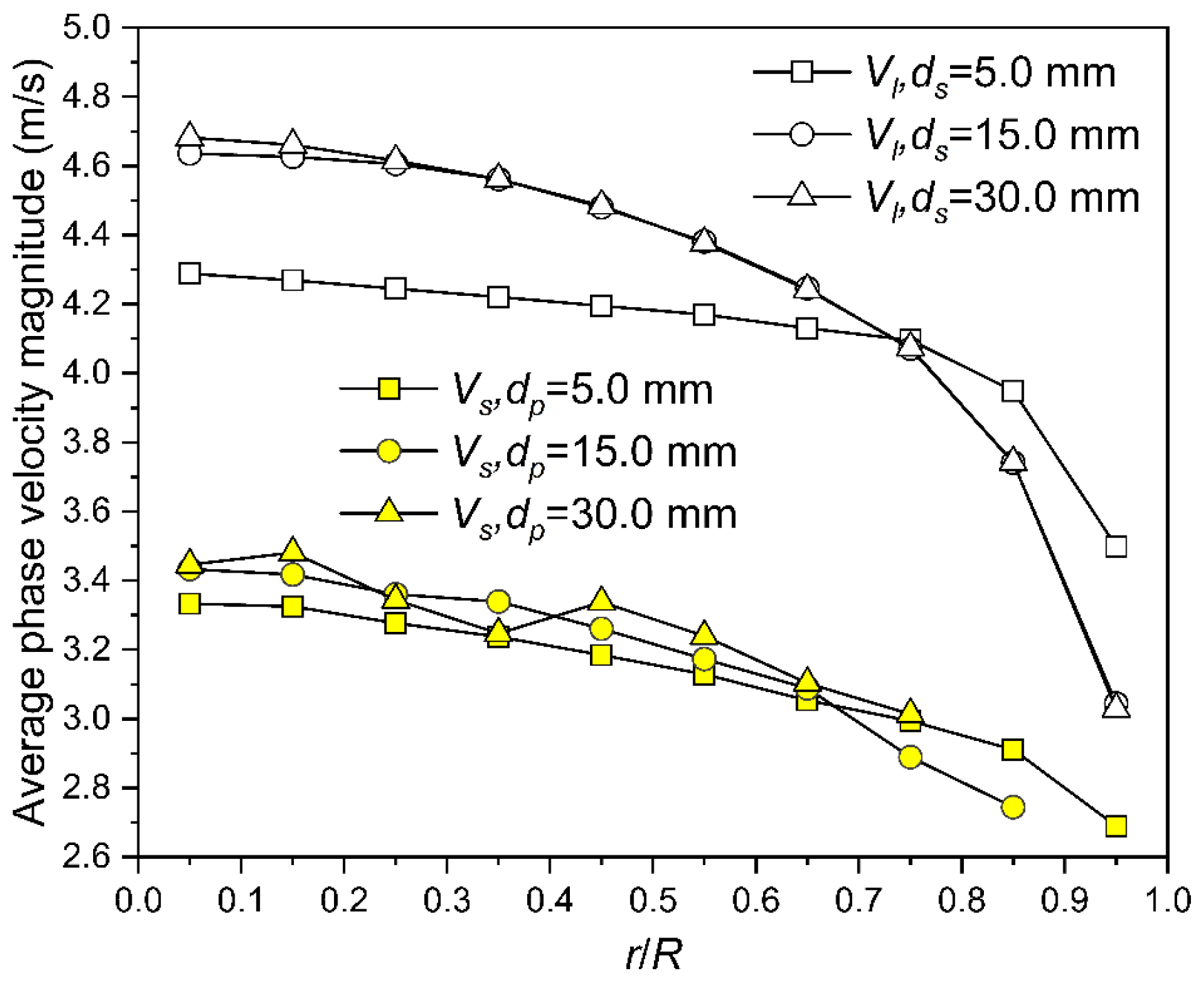
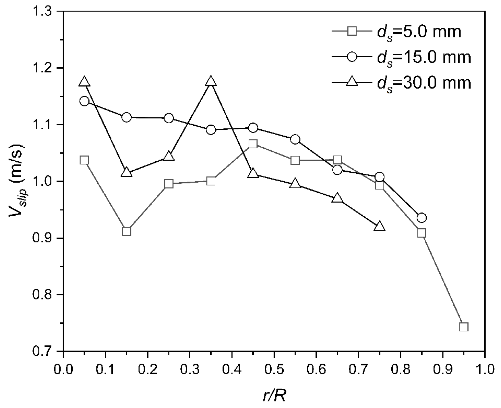
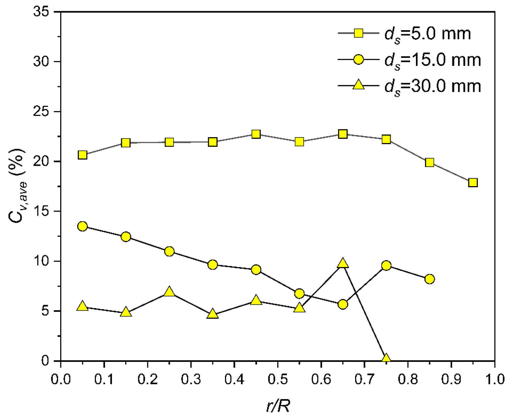
Particle diameter has a significant influence on the rising velocities of seawater and manganese nodules. At the central part of the pipe, the liquid velocity is relatively low for small particles, while high liquid velocity arises near the pipe wall for small particle flow compared to large particle flow. The total pressure drop decreases with the increase of particle size from 5.0 mm to 30.0 mm.

(3)

At different flow velocities, similar seawater velocity distributions are evidenced. The velocity of manganese nodules exhibits the same tendency, and the highest velocity is produced at the pipe axis and then decreases in a radial direction. Increasing initial mixture velocity is beneficial to the transport of manganese nodules, but it will consume more energy and result in the increase of total pressure drop.

(4)

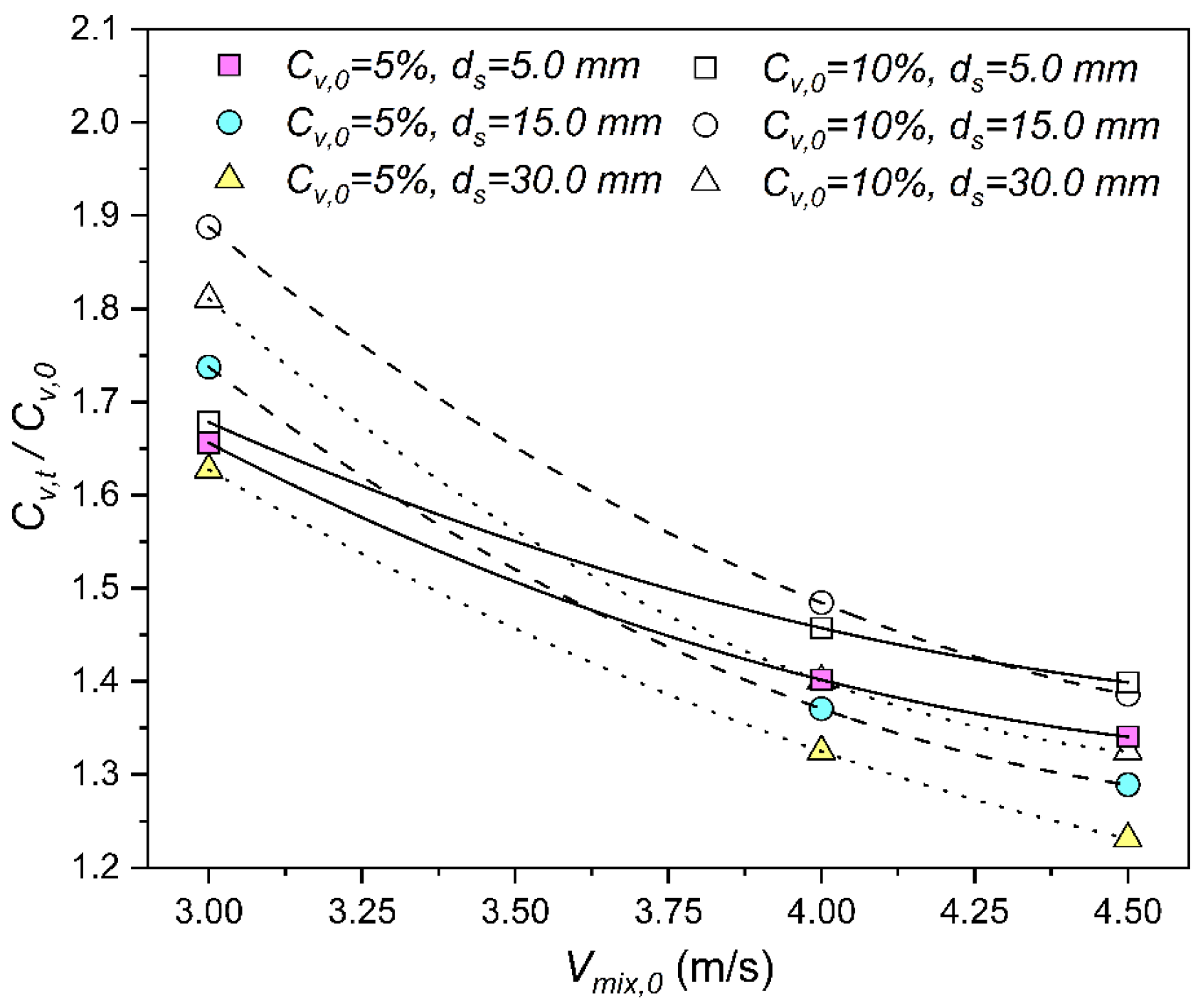
For both small and large particles, the retention ratio declines with increasing initial mixture velocity and decreasing initial solid volume fraction. At an initial mixture velocity of 4.5 m/s, the particles of 30.0 mm in diameter are responsible for the lowest retention ratio, implying a significant effect of the initial mixture velocity on the transport performance.

(5)

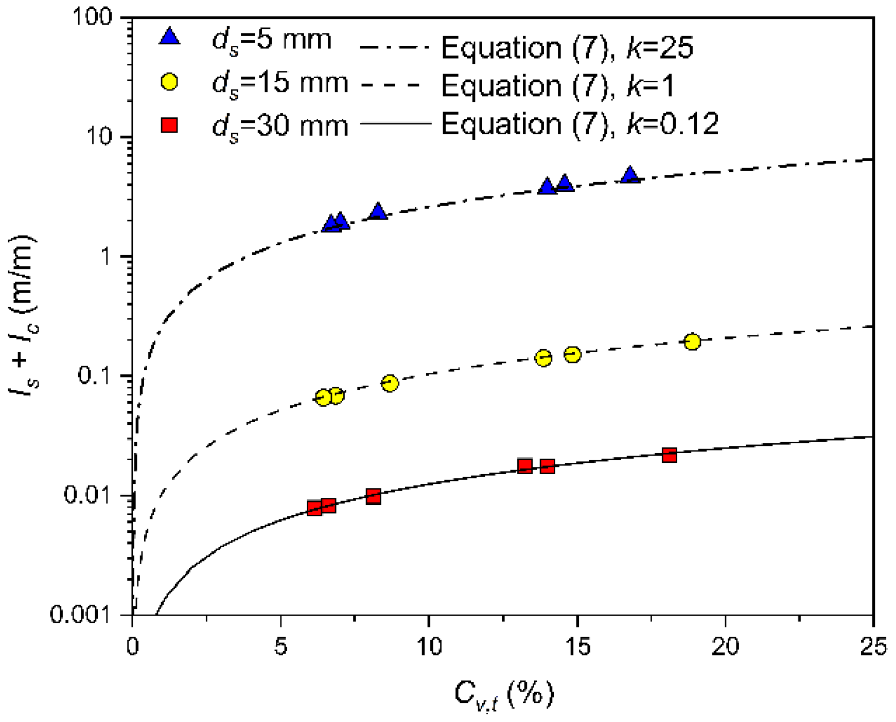
A formula is proposed to describe the pressure drop due to the presence of solid particles and collisions. Combined with the pressure drop formula associated with clean water, the total pressure drop for the hydraulic transportation of solid particles can be well predicted.

References

- Miller, K.A.; Thompson, K.F.; Johnston, P.; Santillo, D. An Overview of Seabed Mining Including the Current State of Development, Environmental Impacts, and Knowledge Gaps. Front. Mar. Sci. 2018, 4, 418. [Google Scholar] [CrossRef]
- Takahashi, H.; Masuyama, T.; Noda, K. Unstable Flow of a Solid-Liquid Mixture in a Horizontal Pipe. Int. J. Multiph. Flow 1989, 15, 831–841. [Google Scholar] [CrossRef]
- Zhou, M.; Wang, S.; Kuang, S.; Luo, K.; Fan, J.; Yu, A. CFD-DEM Modelling of Hydraulic Conveying of Solid Particles in a Vertical Pipe. Powder Technol. 2019, 354, 893–905. [Google Scholar] [CrossRef]
- Singh, J.P.; Kumar, S.; Mohapatra, S.K. Modelling of Two Phase Solid-Liquid Flow in Horizontal Pipe Using Computational Fluid Dynamics Technique. Int. J. Hydrogen Energy 2017, 42, 20133–20137. [Google Scholar] [CrossRef]
- Xia, J.X.; Ni, J.R.; Mendoza, C. Hydraulic Lifting of Manganese Nodules Through a Riser. J. Offshore Mech. Arct. 2004, 126, 72–77. [Google Scholar] [CrossRef]
- Yoon, C.H.; Kang, J.S.; Park, Y.C.; Kim, Y.J.; Park, J.M.; Kwon, S.K. Solid-Liquid Flow Experiment with Real and Artificial Manganese Nodules in Flexible Hoses. In Proceedings of the Eighteenth (2008) International Offshore and Polar Engineering Conference, Vancouver, BC, Canada, 6 July 2008. [Google Scholar]
- Doron, P.; Barnea, D. Pressure Drop and Limit Deposit Velocity for Solid-Liquid Flow in Pipes. Chem. Eng. Sci. 1995, 50, 1595–1604. [Google Scholar] [CrossRef]
- Doron, P.; Simkhis, M.; Barnea, D. Flow of Solid-Liquid Mixtures in Inclined Pipes. Int. J. Multiph. Flow 1997, 23, 313–323. [Google Scholar] [CrossRef]
- Song, Y.; Zhu, X.; Sun, Z.; Tang, D. Experimental Investigation of Particle-Induced Pressure Loss in Solid–Liquid Lifting Pipe. J. Cent. South Univ. 2017, 24, 2114–2120. [Google Scholar] [CrossRef]
- Ravelet, F.; Bakir, F.; Khelladi, S.; Rey, R. Experimental Study of Hydraulic Transport of Large Particles in Horizontal Pipes. Exp. Therm. Fluid Sci. 2013, 45, 187–197. [Google Scholar] [CrossRef] [Green Version]
- Shokri, R.; Nobes, D.S.; Ghaemi, S.; Sanders, R.S. Investigation of Particle-Fluid Interaction at High Reynolds-Number Using PIV/PTV Techniques. In Proceedings of the International Symposium on Turbulence and Shear Flow Phenomena (TSFP-9), Melbourne, Australia, 30 July 2015. [Google Scholar]
- Moliner, C.; Marchelli, F.; Spanachi, N.; Martinez-Felipe, A.; Bosio, B.; Arato, E. CFD Simulation of a Spouted Bed: Comparison between the Discrete Element Method (DEM) and the Two Fluid Model (TFM). Chem. Eng. J. 2019, 377, 120466. [Google Scholar] [CrossRef] [Green Version]
- Chen, X.; Wang, J. A Comparison of Two-Fluid Model, Dense Discrete Particle Model and CFD-DEM Method for Modeling Impinging Gas–Solid Flows. Powder Technol. 2014, 254, 94–102. [Google Scholar] [CrossRef]
- Blais, B.; Lassaigne, M.; Goniva, C.; Fradette, L.; Bertrand, F. Development of an Unresolved CFD–DEM Model for the Flow of Viscous Suspensions and Its Application to Solid–Liquid Mixing. J. Comput. Phys. 2016, 318, 201–221. [Google Scholar] [CrossRef]
- Hua, L.; Lu, L.; Yang, N. Effects of Liquid Property on Onset Velocity of Circulating Fluidization in Liquid-Solid Systems: A CFD-DEM Simulation. Powder Technol. 2020, 364, 622–634. [Google Scholar] [CrossRef]
- Xu, L.; Zhang, Q.; Zheng, J.; Zhao, Y. Numerical Prediction of Erosion in Elbow Based on CFD-DEM Simulation. Powder Technol. 2016, 302, 236–246. [Google Scholar] [CrossRef]
- Chu, K.W.; Wang, B.; Yu, A.B.; Vince, A. CFD-DEM Modelling of Multiphase Flow in Dense Medium Cyclones. Powder Technol. 2009, 193, 235–247. [Google Scholar] [CrossRef]
- Sakai, M.; Abe, M.; Shigeto, Y.; Mizutani, S.; Takahashi, H.; Viré, A.; Percival, J.R.; Xiang, J.; Pain, C.C. Verification and Validation of a Coarse Grain Model of the DEM in a Bubbling Fluidized Bed. Chem. Eng. J. 2014, 244, 33–43. [Google Scholar] [CrossRef]
- Cheng, J.; Zhang, N.; Li, Z.; Dou, Y.; Cao, Y. Erosion Failure of Horizontal Pipe Reducing Wall in Power-Law Fluid Containing Particles via CFD–DEM Coupling Method. J. Fail. Anal. Prev. 2017, 17, 1067–1080. [Google Scholar] [CrossRef]
- Alobaid, F.; Ströhle, J.; Epple, B. Extended CFD/DEM Model for the Simulation of Circulating Fluidized Bed. Adv. Powder Technol. 2013, 24, 403–415. [Google Scholar] [CrossRef]
- Yang, X.-D.; Zhao, L.-L.; Li, H.-X.; Liu, C.-S.; Hu, E.-Y.; Li, Y.-W.; Hou, Q.-F. DEM Study of Particles Flow on an Industrial-Scale Roller Screen. Adv. Powder Technol. 2020, 31, 4445–4456. [Google Scholar] [CrossRef]
- Zhou, Z.Y.; Kuang, S.B.; Chu, K.W.; Yu, A.B. Discrete Particle Simulation of Particle–Fluid Flow: Model Formulations and Their Applicability. J. Fluid Mech. 2010, 661, 482–510. [Google Scholar] [CrossRef]
- Rubinow, S.I.; Keller, J.B. The Transverse Force on a Spinning Sphere Moving in a Viscous Fluid. J. Fluid Mech. 1961, 11, 447. [Google Scholar] [CrossRef]
- Saffman, P.G. The Lift on a Small Sphere in a Slow Shear Flow. J. Fluid Mech. 1965, 22, 385–400. [Google Scholar] [CrossRef] [Green Version]
- Okhovat-Alavian, S.M.; Shabanian, J.; Norouzi, H.R.; Zarghami, R.; Chaouki, J.; Mostoufi, N. Effect of Interparticle Force on Gas Dynamics in a Bubbling Gas–Solid Fluidized Bed: A CFD-DEM Study. Chem. Eng. Res. Des. 2019, 152, 348–362. [Google Scholar] [CrossRef]
- Burke, S.P.; Plummer, W.B. Gas Flow through Packed Columns. Ind. Eng. Chem. 1928, 20, 1196–1200. [Google Scholar] [CrossRef]
- Li, Y.W.; Liu, S.J.; Hu, X.Z. Research on Reflux in Deep-Sea Mining Pump Based on DEM-CFD. Mar. Georesour. Geotechnol. 2020, 38, 744–752. [Google Scholar]
- Liu, Y.; Chen, L. Numerical Investigation on the Pressure Loss of Coarse Particles Hydraulic Lifting in the Riser with the Lateral Vibration. Powder Technol. 2020, 367, 105–114. [Google Scholar] [CrossRef]
- Hong, S.; Choi, J.; Yang, C.-K. Experimental Study on Solid-Water Slurry Flow in Vertical Pipe by Using Ptv Method. In Proceedings of the Twelfth (2002) International Offshore and Polar Engineering Conference, Kitakyushu, Japan, 26 May 2002. [Google Scholar]
- Friman Peretz, M.; Levy, A. Bends Pressure Drop in Hydraulic Conveying. Adv. Powder Technol. 2019, 30, 1484–1493. [Google Scholar] [CrossRef]