Image Classification of Pests with Residual Neural Network Based on Transfer Learning

Abstract

Agriculture is regarded as one of the key food sources for humans throughout history. In some countries, more than 90% of the population lives on agriculture. However, pests are regarded as one of the major causes of crop loss worldwide. Accurate and automated technology to classify pests can help pest detection with great significance for early preventive measures. This paper proposes the solution of a residual convolutional neural network for pest identification based on transfer learning. The IP102 agricultural pest image dataset was adopted as the experimental dataset to achieve data augmentation through random cropping, color transformation, CutMix and other operations. The processing technology can bring strong robustness to the affecting factors such as shooting angles, light and color changes. The experiment in this study compared the ResNeXt-50 (32 × 4d) model in terms of classification accuracy with different combinations of learning rate, transfer learning and data augmentation. In addition, the experiment compared the effects of data enhancement on the classification performance of different samples. The results show that the model classification effect based on transfer learning is generally superior to that based on new learning. Compared with new learning, transfer learning can greatly improve the model recognition ability and significantly reduce the training time to achieve the same classification accuracy. It is also very important to choose the appropriate data augmentation technology to improve classification accuracy. The accuracy rate of classification can reach 86.95% based on the combination of transfer learning + fine-tuning and CutMix. Compared to the original model, the accuracy of classification of some smaller samples was significantly improved. Compared with the relevant studies based on the same dataset, the method in this paper can achieve higher classification accuracy for more effective application in the field of pest classification.

1. Introduction

Pests are regarded as one of the leading causes of crop loss in the world [1]. Some crops such as rice and wheat are prone to being destroyed by pests, resulting in unstable yield and poor quality as well as huge economic losses to farmers. Therefore, how to protect crops from pests has become a necessary research area to maintain and even improve yield and quality. It is also vital for food security and agricultural economic development [2]. How to classify and identify pests is fundamental for pest monitoring and forecasting so as to prevent pests from further damaging crops [3]. Therefore, it is necessary to find an efficient, fast and automatic method of achieving pest classification.

The traditional manual approach is very time-consuming and labor-intensive since the pest morphology is so similar that professional knowledge is needed [4]. Furthermore, the existing technicians capable of classification cannot meet the needs of gradually expanding demands in terms of capability and quantity. Pest classification based on machine learning needs careful selection of features for different species. However, due to the numerous types of pests, the features of metamorphic development and the complicated crop environments, it is very difficult to identify the characteristics through artificial selection and meet the modern needs of applications [5]. With the great success of deep learning in multiple image processing fields and the rapidly increasing popularity of high-quality image capture devices [6,7,8,9,10], an automated pest identification system based on deep learning image processing is expected to be the best solution to reduce labor costs and improve classification performance [11,12,13,14,15]. Convolutional neural networks (CNNs) have also achieved breakthroughs in many fields, so the CNN-based image classification model is also considered significant. Research has recently been conducted in the field of pest classification. The CNN ensemble model proposed by Ung et al. including a fine-grained model, attention mechanism and feature pyramid design has achieved accuracy as high as 74.13% and 99.78% in the IP102 dataset [16] and D0 dataset [17]. The integrated model SMPEnsemble [18] proposed by Ayan et al. based on the training of seven common CNN models has achieved accuracy of 67.13% and 95.15% in the IP102 dataset [16] and D0 dataset [17]. Nanni et al. adopted an ensemble model [19] of six CNNs and carried out the optimization by improving the DGrad and Adam algorithms [20], which achieved accuracy of 95.52%, 75.11% and 99.81% in the Deng dataset [21], IP102 dataset [16] and D0 dataset [17], respectively. The specific accuracy of each model is shown in

Table 1. The comparative result with related work.

Related Work	Model	IP102 [16]	D0 [17]
[18]	GAEnesmble	67.1%	98.8%
[18]	SMPEnsemble	66.2%	98.4%
[21]	HierarchicalModel
[19]	SaliencyEnsemble	61.9%
[22]	Multiple Instance Learning	60.7%
[18]	SMPEnsemble	66.2%	98.4%
[16]	DeepFeature	49.5%
[23]	FR·ResNet	55.2%
[22]	Inception-V4	48.2%
[22]	ResNet50	49.4%
[22]	MobileNet-B0	53.0%
[22]	DenseNet121	61.1%
[22]	EfficientNet-B0	60.7%
[17]	Multi-level framework		89.3%
[24]	CNN		90.0%
[25]	Deep CNN with augmentation		96.0%
[26]	Ensemble model	74.1%	99.8%
[27]	Inception V3	81.7%
[27]	VGG19	80%
[28]	Ensemble model	74.11%
[29]	STN-ResNest	73.29%
Presented Work	ResNeXt-50 (32 × 4d)	86.9%

.

These results show that the scheme of automatic feature extraction based on a CNN is more effective than the traditional machine learning of manually selecting features in the field of agricultural pest classification. As shown in Table 1, the current research on pest classification based on the CNN model mostly adopts the scheme of ensemble model, and there is no clear solution to the problem of small database size and inability to fully meet the training requirements of the model. In addition, there is a wide range of biological similarities between pests. It is necessary to adopt an effective method to help the model fully learn the deep features of the samples.

In this paper, we propose a convolution neural network pest classification method based on transfer learning and data enhancement. Based on the complexity of the experiment, we adopted three combined learning methods (new learning, transfer learning + freezing, transfer learning + fine-tuning), three data augmentation methods (no enhancement, cropping + toning + dimming, CutMix + cropping + toning + dimming) and three groups of initial learning rates (0.0001, 0.0005, 0.001) to conduct a total of 27 combined experiments. Then, we evaluated the method performance on the IP102 dataset and compared results with several popular models. The experimental results show that method can achieve better performance on the IP102 dataset.

2. Model

2.1. Convolutional Neural Network

With the rapid development of hardware and computing technology accelerated by GPUs in recent years, the problem of high computational cost of convolutional neural networks (CNNs) has been gradually solved, which enables them to be applied in more fields. At present, CNNs are among the most popular deep learning models. Although different CNNs have different structures, they all consist of three specialized parts: the convolutional layer, pooling layer and fully connected layer. The main function of the convolutional layer and pooling layer is to extract features. The convolutional layer extracts regional features from the input of the previous layer through the convolution operator and kernel function then conveys these features to the pooling layer to reduce the dimensionality by means of operations such as maximum, minimum and average pooling. Finally, it completes the mapping from features to labels through one or more fully connected layers.

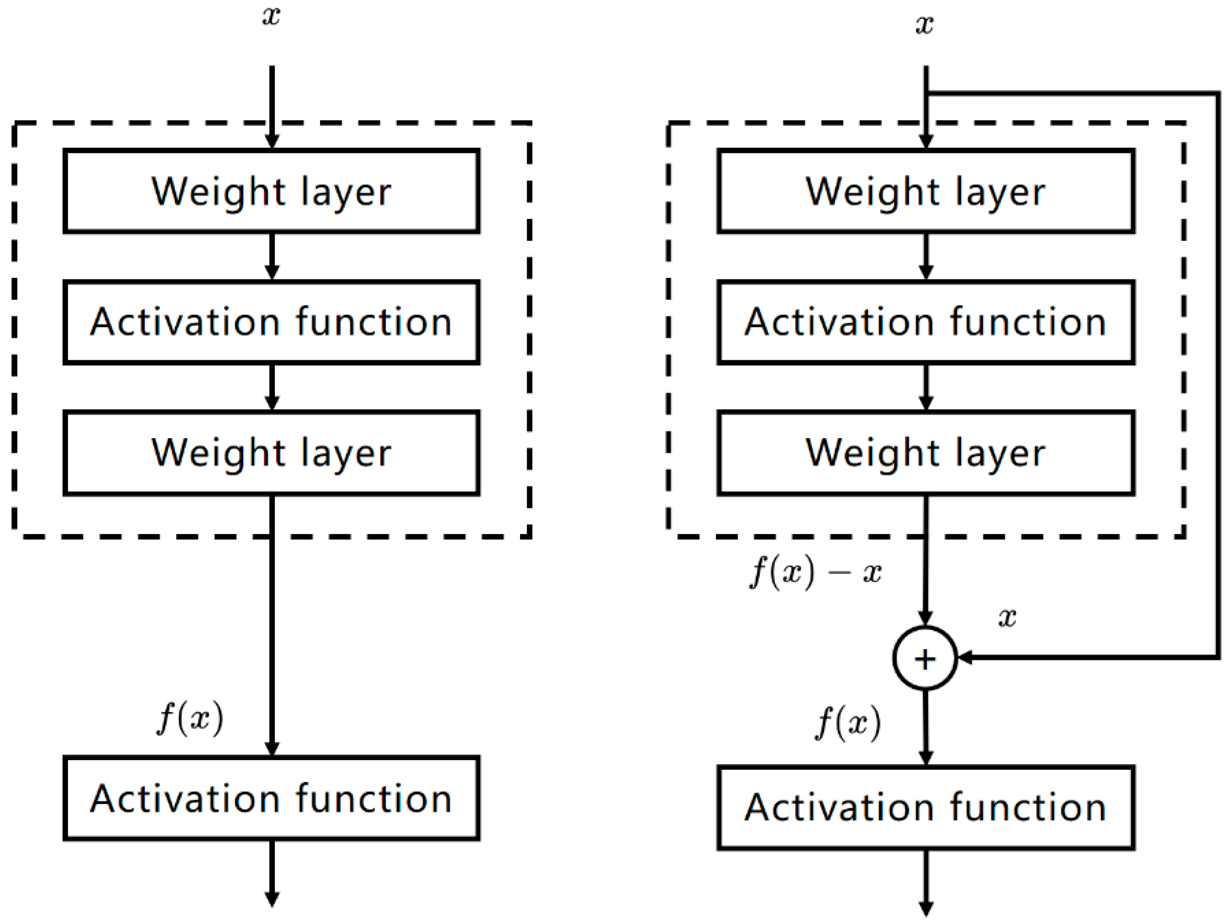
2.2. ResNet

ResNet [30] is a residual CNN proposed by He et al. with the core idea of allowing the original input information to be passed directly to the subsequent network. The residual blocks [30] are designed based on the aforesaid concept, and the structure is shown in Figure 1. The innovative design allows the networks with residual blocks to be deeper with less possibility of gradient vanishing because the original input in the residual block can be propagated forward faster through the identity mapping.

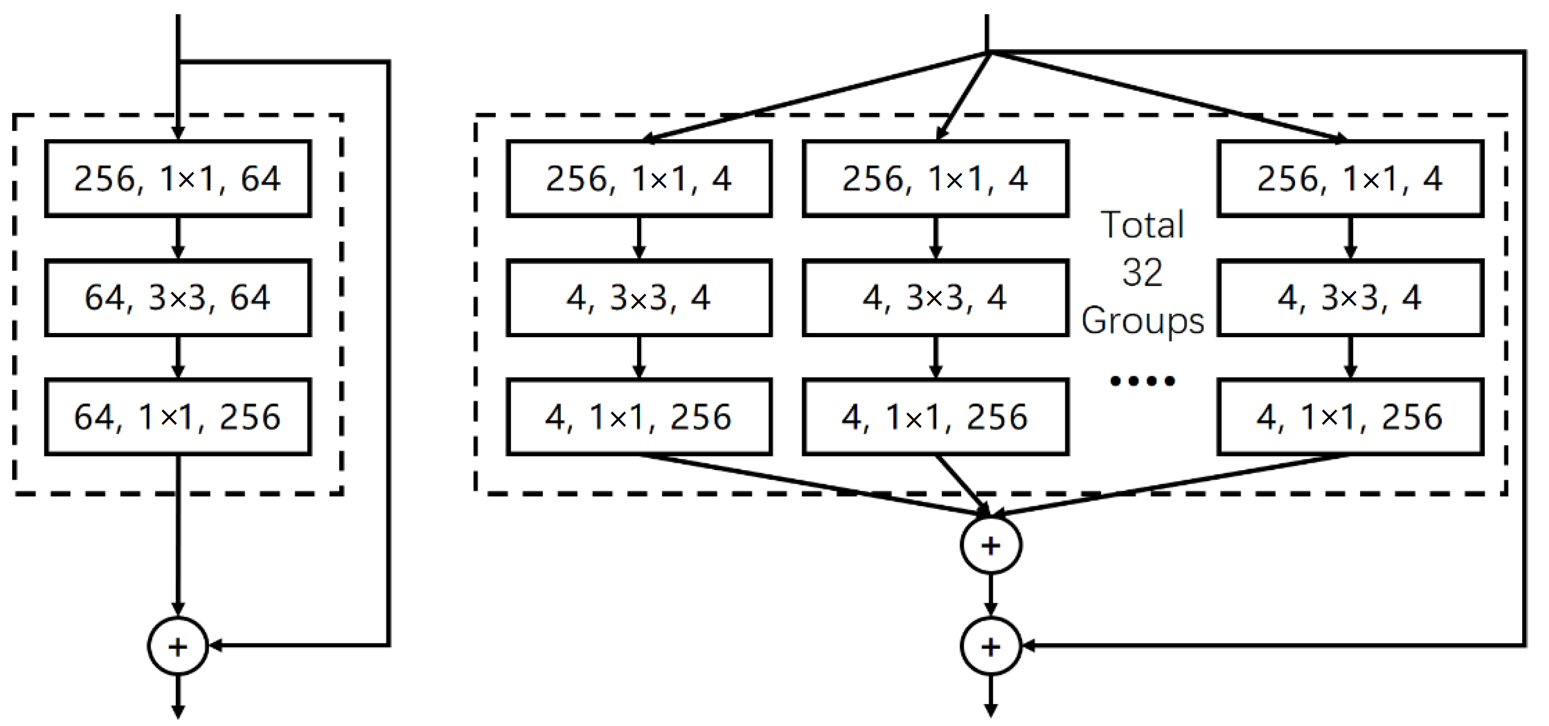
2.3. ResNeXt

ResNeXt [31] is proposed by He et al. as an improvement of ResNet. Firstly, it retains the design concept of the residual block in ResNet and improves the ResNet residual blocks by introducing group convolution so as to obtain ResNeXt residual blocks [31]. The structure of ResNet and ResNeXt residual blocks is shown in Figure 2. Secondly, it broadens the cardinality of the network by referring to the concept of split–transform–merge in Inception [32]. Finally, it adopts the concise design principle of VGG [33] to overcome the disadvantages of Inception [32] convolution kernel parameters which are too complicated to control.

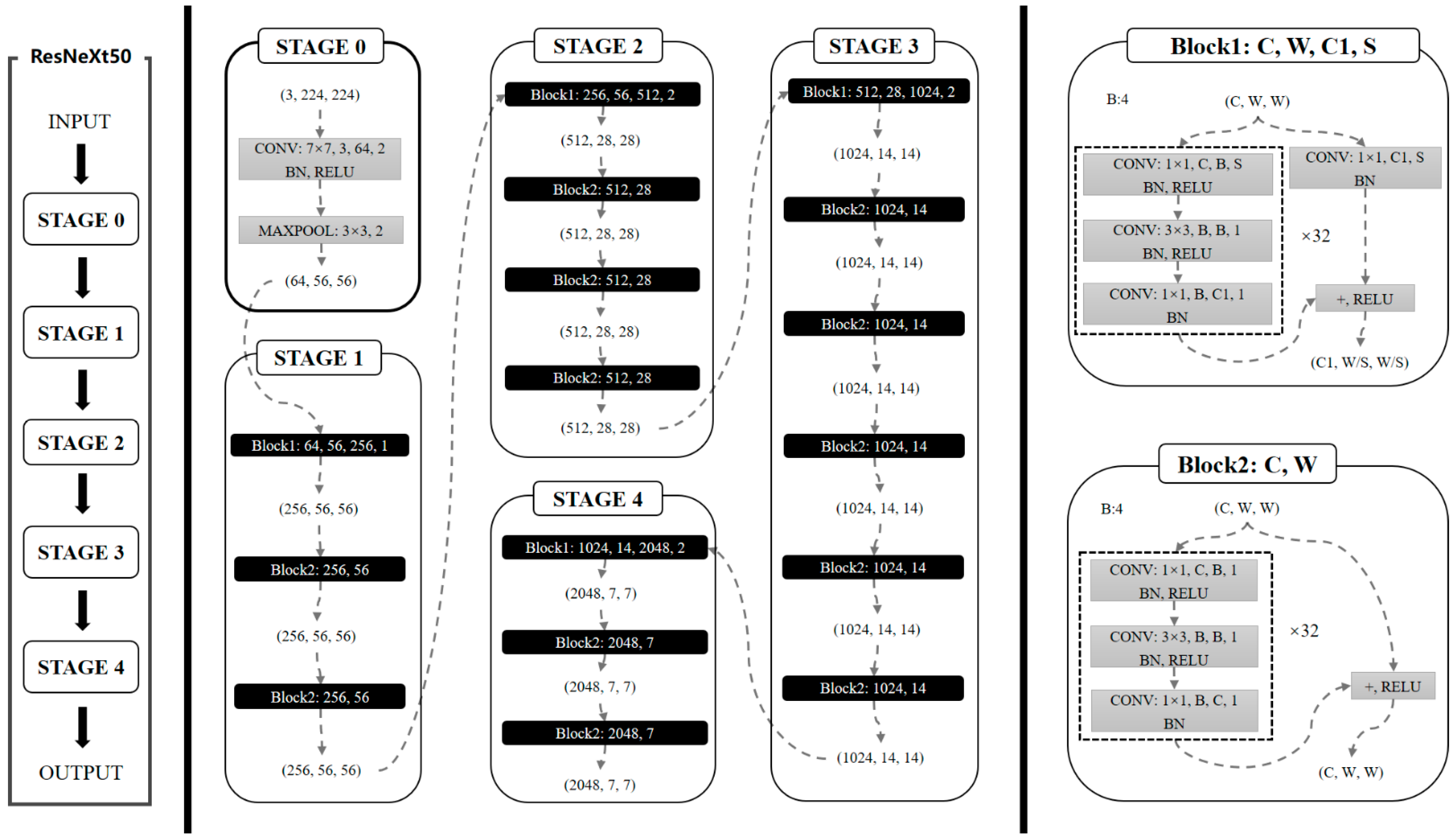
2.4. Model Structure

The ResNeXt-50 (32 × 4d) [31] model structure was adopted in this study. This structure is divided into six layers. The first layer consists of one initialized convolutional layer for preliminary feature extraction; the second layer consists of one maximum pooling layer and three ResNeXt residual blocks stacked for shallow feature extraction; the third to fifth layers consist of 4, 6, and 3 repeated stacked ResNeXt residual blocks, respectively, the size of which is reduced layer-by-layer for deep feature extraction; the sixth layer is used to calculate the full connection from the convolution layer features to the sample category mapping, and SoftMax is adopted to calculate the losses. The specific model structure is shown in Figure 3.

3. Materials and Methods

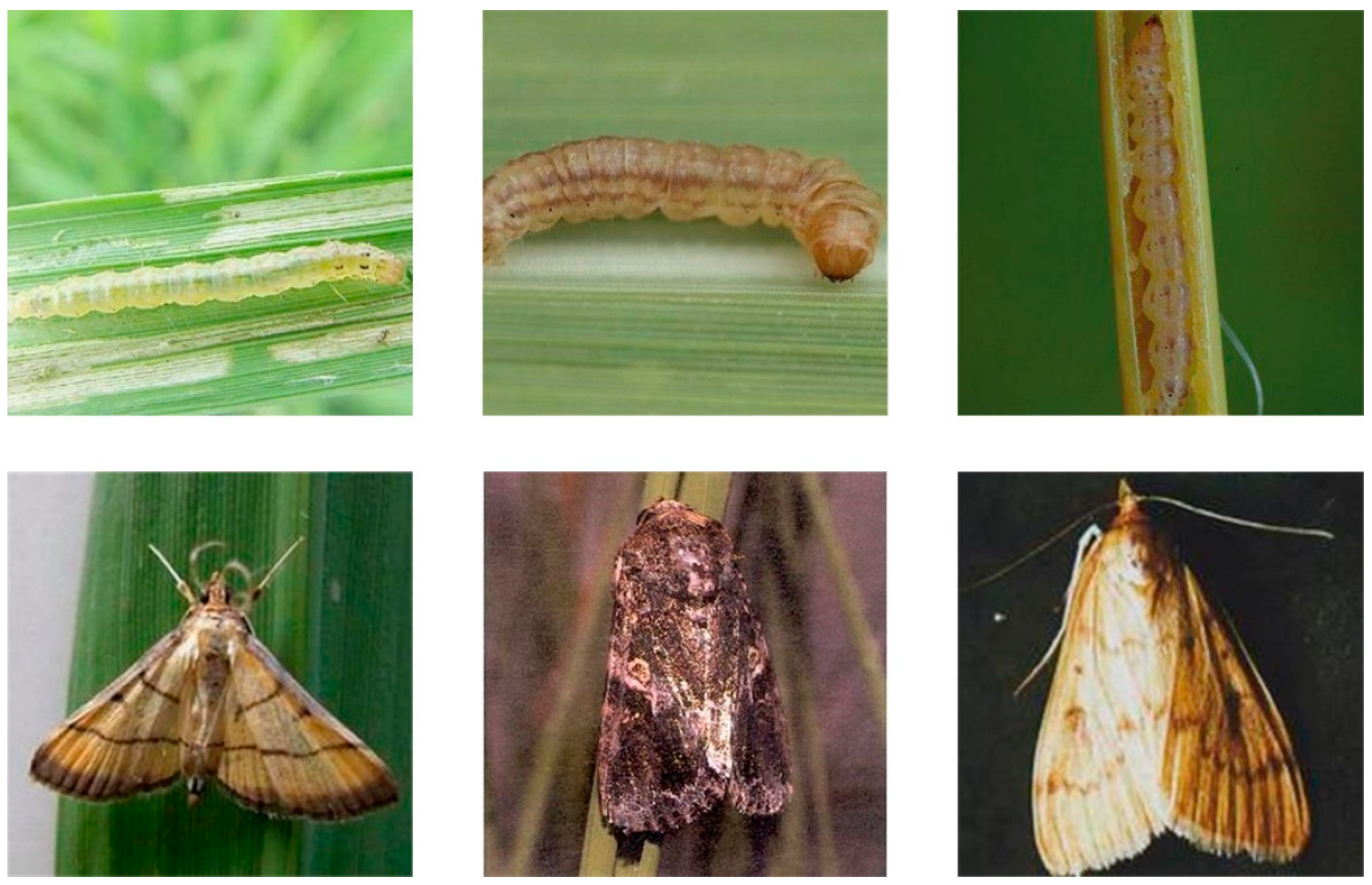
3.1. Dataset

The experiment adopted the IP102 pest dataset [16], a large-scale benchmark dataset proposed by Wu et al., which contains 75,222 images of 102 pest species. All the pests are labelled by hierarchical taxonomy, and each pest is classified into a superclass mapping the crop type to be preyed upon and a subclass marked as the type to destroy crops. The dataset was partitioned into two subsets according to 8:2. The training and testing sets were split at a subclass level. This dataset is somewhat challenging [23]. First of all, most pests are featured with metamorphosis, so there are still some differences among the same category of pests. Secondly, different species of pests have certain similarities in the same morphological period. Thirdly, the dataset contains a large number of small-sized pests in the complicated environment. Finally, this dataset can reflect the real quantity and distribution of pests to a certain extent; however, there is a serious imbalance featured with natural long-tailed distribution in terms of sample numbers among different pest species [26]. Sample images from the dataset are shown in Figure 4.

3.2. Transfer Learning

Transfer learning is a kind of learning method based on existing knowledge to solve the problems so as to transfer knowledge between different and relevant fields [34]. In terms of the CNN, transfer learning aims to successfully apply the “knowledge” trained on a specific dataset to a new domain; that is to say, it aims to use similar datasets to train the model to help the model learn general “knowledge” and apply it to the target problem.

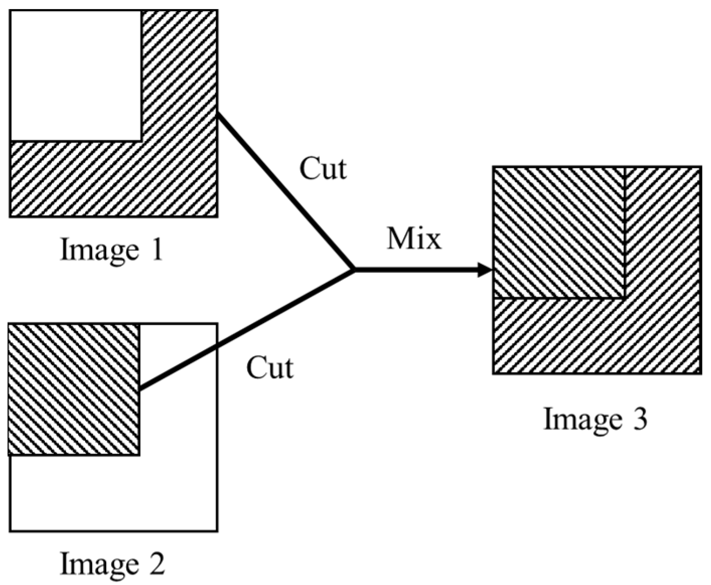
3.3. CutMix

The CutMix method is a regularization strategy for the CNN classification model, and it performs sample transformation by cutting and splicing two training images [35]. As shown in Figure 5, a local area of a training image is removed, and the removed area is filled with a patch from another image. The category label of the image is mixed based on the area ratio of the original and patch images.

3.4. Model Optimization

The model adopts CrossEntropy to calculate the classification loss, so as to calculate the similarity between the SoftMax results from the model and the true probability distribution of the target. Moreover, L2 regularization is added to penalize the weight parameters and mitigate the overfitting. The mathematical formula is shown in Equation (1).

$$J\left(\theta \right)=-{\displaystyle \sum p}\left(x\right){\log }_{2}q\left(x\right)+\lambda {\parallel \theta \parallel }^2$$

(1)

wherein $p(x)$ is the target probability distribution; $q(x)$ is the prediction distribution; $\theta$ is the weight parameter; $\lambda$ is the regularization coefficient; ${\parallel \theta \parallel }^2$ is the regularization added to prevent overfitting.

The parameter optimization is actually the process of iteratively minimizing the loss function. The Adam algorithm [20] was adopted in this study to optimize the model parameters. In terms of the learning rate update strategy, the cosine annealing algorithm was adopted to iteratively update the network weights through the training data. The mathematical formula is shown in Equation (2). The Adam optimizer has the advantages of both AdaGrad [36] and RMSProp algorithms, so it can adaptively maintain the learning rate to improve the performance of sparse gradients and anti-noise with fewer parameters and higher efficiency. The calculation steps are as follows:

$${new}_{lr}={\mathrm{eta}}_{\min }+0.5\ast ({\mathrm{initial}}_{lr0}-{\mathrm{eta}}_{\min })\times (1+\cos (\frac{\mathrm{epoch}}{T_{\max }}\pi \left)\right)$$

(2)

wherein $lr$ is the decayed learning rate, $l{r}_0$ is the initial learning rate, $\mathrm{epoch}$ is the current number of iterations.

4. Results and Discussion

4.1. Results

Considering the hardware performance and training time, the batch size for both testing and training is set to 32, the test interval and display interval are set to 1 cycle and the maximum number of training rounds is set to 110 cycles. The data of experiment are shown in

Table 2. Loss and accuracy of model training and test.

Group ID	Learning Method	Data Augmentation	Learning Rate	Training Loss	Test Losses	Training Accuracy	Testing Accuracy
1	New Learning	A	0.0001	0.0172	3.4692	99.30%	48.63%
2			0.0005	0.0146	4.5273	99.46%	49.27%
3			0.0010	0.0113	4.4682	99.59%	53.78%
4		B	0.0001	0.6247	1.4675	82.14%	64.83%
5			0.0005	0.4834	1.5741	84.83%	66.06%
6			0.0010	0.4653	1.5488	85.73%	67.16%
7		C	0.0001	2.3377	1.4835	47.71%	60.01%
8			0.0005	2.0608	1.2979	56.50%	68.11%
9			0.0010	1.9613	1.1765	57.88%	69.75%
10	Transfer Learning + Freeze	A	0.0001	0.0040	1.8967	99.81%	71.42%
11			0.0005	0.2828	1.3341	91.72%	67.97%
12			0.0010	0.1887	1.7385	94.43%	66.24%
13		B	0.0001	1.1873	1.1250	65.98%	67.99%
14			0.0005	0.9802	1.1283	70.89%	68.05%
15			0.0010	0.9170	1.1823	72.83%	69.13%
16		C	0.0001	2.4079	1.2961	47.60%	66.65%
17			0.0005	2.2698	1.1673	51.19%	69.01%
18			0.0010	2.2559	1.1121	51.86%	70.14%
19	Transfer learning + Fine-tuning	A	0.0001	0.0030	1.8918	99.85%	72.64%
20			0.0005	0.0042	2.5541	99.82%	67.27%
21			0.0010	0.0056	2.9742	99.75%	63.55%
22		B	0.0001	0.1768	1.5413	94.22%	73.86%
23			0.0005	0.2522	1.5639	91.74%	72.33%
24			0.0010	0.3476	1.4343	88.96%	71.99%
25		C	0.0001	1.0959	0.5157	79.11%	86.95%
26			0.0005	1.2358	0.6788	75.64%	81.50%
27			0.0010	1.5114	0.7895	69.26%	77.06%

Note: A, B, and C are data augmentation methods: A means no enhancement to transform the input image into a 224 × 224 pixel image; B means basic enhancement with basic transformation operations such as rotation, toning and stretching of the input image; C means CutMix to enhance the input sample image first and then conduct the CutMix operation based on the maximum mixing number of 2. Data enhancement refers to the direct sample modification during the model training, which has no influence on the quantity and distribution of the samples. New learning refers to all parameters of the model being randomly generated, and the model is only trained in the target dataset; transfer learning + freezing refers to the model being pre-trained in similar datasets first, then the pre-training parameters are frozen during the training in the target dataset and only the fully connected output layer is trained; transfer learning + fine-tuning refers to the model being pre-trained in a similar dataset first, and then all the model parameters are trained in the target dataset, including the parameters of the pre-training and the newly added fully connected layers.

.

We conducted experiments to compare the performance of our proposed scheme with different models.

Table 3. The comparison among different proposed models.

Model	Accuracy	Average Precision	Average Recall	Average F1 Score
Densenet121	81.55%	78.03%	73.93%	75.92%
Efficientnet-B0	80.28%	78.75%	73.66%	76.12%
VGG19	78.80%	78.21%	74.54%	76.33%
ResNet-50	71.20%	70.06%	65.39%	67.64%
ResNeSt-50	80.28%	78.47%	71.47%	74.81%
ResNeXt-50 (32 × 4d)	86.50%	84.62%	85.55%	85.08%

presents the results of those models on IP102. Among those models, ResNeXt-50 (32 × 4d) achieves the best performance for accuracy, average precision, average recall and average F1 scores, an improvement of 4.95 percentage points on the accuracy of DenseNet121.

4.2. Discussion

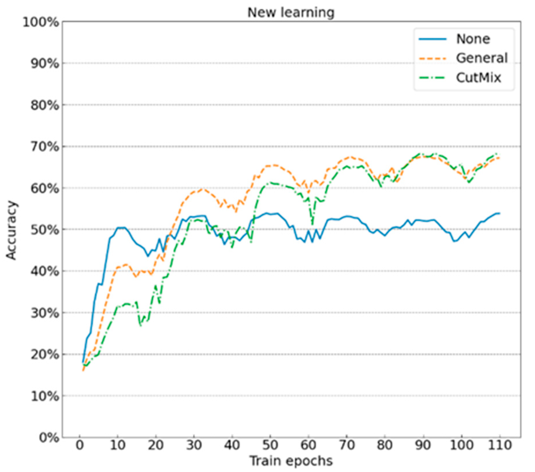
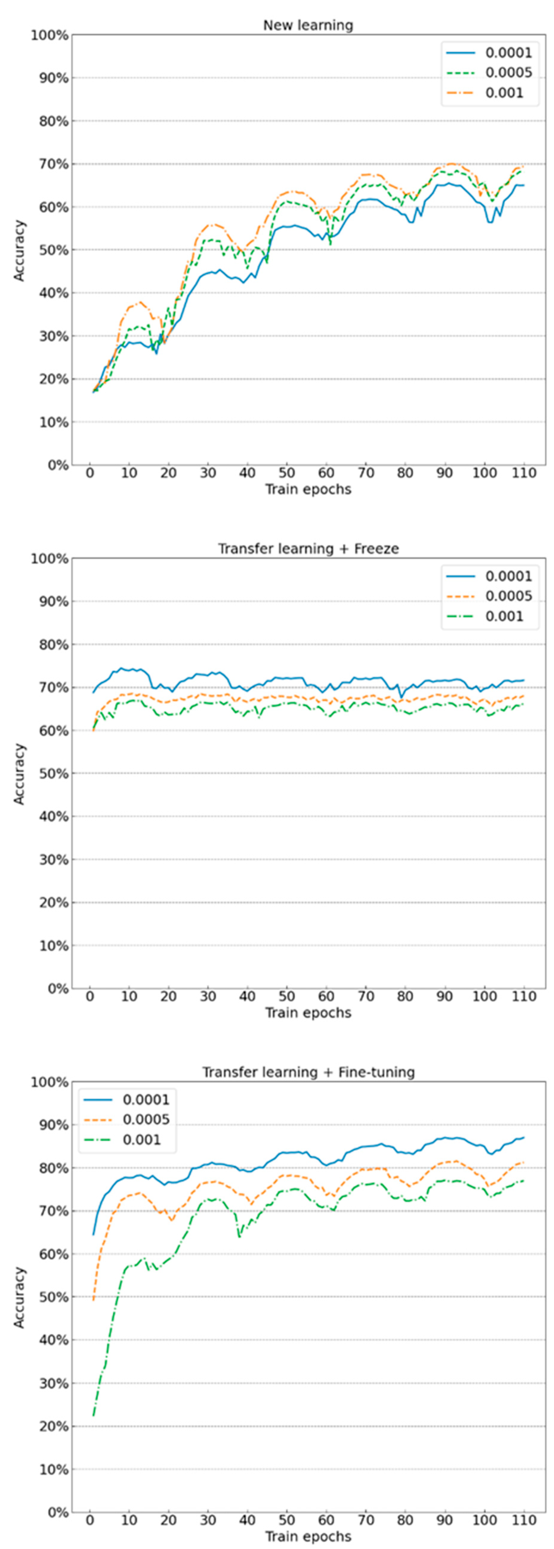
4.2.1. Learning Rate

During the training process, the learning rate changes dynamically as per the cosine annealing algorithm. The reset learning rate period is set to 10, that is, the learning rate changes periodically based on a cosine function whose period is 20, maximum value is initial learning rate and the minimum value is 0. The curve first falls and then rises within a period.

As shown in Figure 6, the learning rate greatly affects the training and testing results. With the new learning method, all parameters are randomly generated by truncated normal distribution, and the higher learning rate enables the training to quickly approach the optimal solution so that higher training and testing accuracy can be obtained with the same rounds of training. For example, in the ninth group of the experiment, the initial learning rate is 0.001. After 110 rounds of training, the training and testing accuracy rates reach 57.88% and 69.75%, respectively, about 5% higher on average than other experiments under the same conditions.

With the method of transfer learning, the model is close to the optimal solution at the initial moment of training since the model owns a certain pre-training “knowledge” in advance. The higher learning rate is prone to skip the optimal solution, resulting in low classification accuracy or severe fluctuations. When the combination of transfer learning + freezing is adopted, the part of feature extraction does not get involved in the learning, so it is less probably affected by the learning rate than the combination of transfer learning + fine-tuning. All groups of experiments with the learning rate of 0.0001 (experiment No.: 10 and 25) indicate good performance with accuracy of 86.95% after 110 periods of training. The results show that better training results can be achieved if the initial learning rate of the model with transfer learning is set to 0.5 or 0.1 times of the new learning.

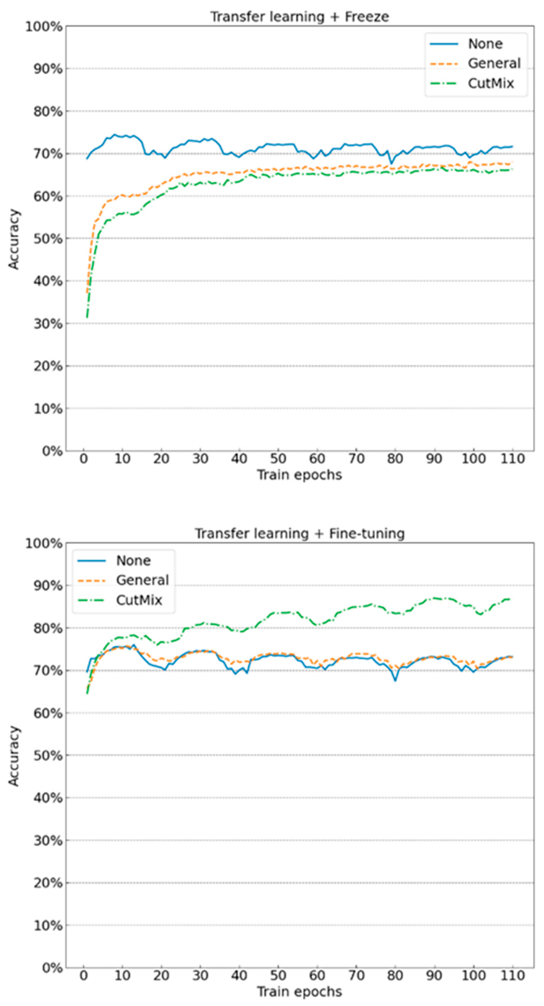
4.2.2. Data Augmentation

As shown in Figure 7, the selection of appropriate data augmentation can significantly improve the classification effect of the model. When the new learning is adopted, since the model needs to learn the “knowledge” from the target dataset which has a small capacity, it cannot fully meet the needs of model training. Therefore, the experimental results show obvious overfitting without the data augmentation. For example, in the third group of experiments, the training accuracy rate reaches 99.59%, but the accuracy is only 53.78%. After the data enhancement is adopted, the accuracy rate is greatly improved, and the overfitting is significantly reduced. As another example, in the sixth group of the experiment, the training and testing accuracies reach 85.73% and 67.16%, respectively. The adoption of base augmentation or CutMix augmentation has no significant influence on the results of new learning model. It is expected that the learning speed is slow due to the high complexity of CutMix enhancement in the early training process.

Freezing and fine-tuning have different options for data augmentation in terms of the experiments of transfer learning. When transfer learning + freezing is adopted, since the feature extraction does not get involved in the training, the data augmentation increases the possibility of misclassification of the fully connected layer, so the classification effect without data augmentation is the optimal solution. When transfer learning + fine-tuning is adopted, the feature extraction layer is pre-trained in similar datasets, and the basic data enhancement has no obvious influence on the experiment results. Taking the 19th and 22nd group experiments as the example, the accuracy rates are 72.64% and 73.86%, respectively. When more complicated data augmentation such as CutMix is adopted, it results in a better learning effect. As another example, in the 25th group of the experiment, the training and test accuracies reach 79.11% and 86.95%, respectively. Therefore, when the model has a certain “basic knowledge”, more complicated data augmentation helps the model learn at a further level.

Figure 8 shows the accuracy of different classifications in the IP102 dataset with different data enhancements. In terms of minimal size of samples, the model performance is not be significantly improved regardless of method. For example, the results of three experiments in the first group are very similar. When there is a certain sample size, data enhancement can significantly improve the classification performance of the model, especially as CutMix can provide better performance than ordinary data enhancement. However, in the case of sufficient sample size, although the data enhancement can improve the sample performance to a certain degree, the effect is not very obvious because the original samples can meet the needs of model training. Therefore, data augmentation is of great significance for helping the model learn a certain number of samples which are insufficient for model training.

4.2.3. Transfer Learning

As shown in Figure 9, the adoption of transfer learning can significantly improve the classification performance of the model. With the new learning method, the model cannot be fully trained due to insufficient number of samples, so the experiment results have the obvious problem of overfitting. Take the ninth group of experiment as the example, the training accuracy rate has reaches as high as 99.59%, while the test accuracy rate is only 53.78%. With the help of pre-trained “knowledge”, the model adopting transfer learning significantly improves classification accuracy compared to the new learning model, and the time needed for the same accuracy is greatly reduced. When comparing the effects of freezing and fine-tuning on transfer learning, when the freezing model is adopted for training, the parameters in the feature extraction are not involved in the training, so the classification accuracy rate enters a relatively stable state when the parameters of the fully connected layer are fully trained. Due to the fewer parameters involved in the training, the model training time is greatly reduced compared to the new learning and fine-tuning methods. The fine-tuning model receives finer learning based on the original “knowledge”, so it has a higher classification accuracy than the freezing model.

In conclusion, since the dataset is relatively small compared to the model, the new learning model cannot fully learn the features of all samples, so the classification accuracy is lower than that of the transfer learning model. Due to the differences between the datasets, fine-tuning needs to be adopted for different datasets in the case of transfer learning.

5. Conclusions

Since the traditional pest classification method has many problems such as hard feature extraction and small size of data sample, the transfer learning method and a residual CNN were adopted in this study to classify the IP102 pest dataset, and the influence of factors on the model performance such as the learning method, data enhancement and learning rate was compared and analyzed. The conclusions are drawn as follows:

• Compared with other CNNs, the residual CNN can achieve better extraction of pest features. Compared with other research results, it has better classification performance with the average recognition accuracy as high as more than 70%;
• Learning rate has a greater influence than the data augmentation on model training stability. The selection of appropriate learning rate can expedite the model convergence so that the model can approach the optimal solution at a faster speed. When the new learning method is adopted, a larger learning rate should be adopted to expedite the learning speed of the model; when the transfer learning method is adopted, a small learning rate should be adopted to prevent the optimal solution being skipped. If an improper learning rate is selected, the training effect is greatly influenced, and the model even diverges in severe cases;
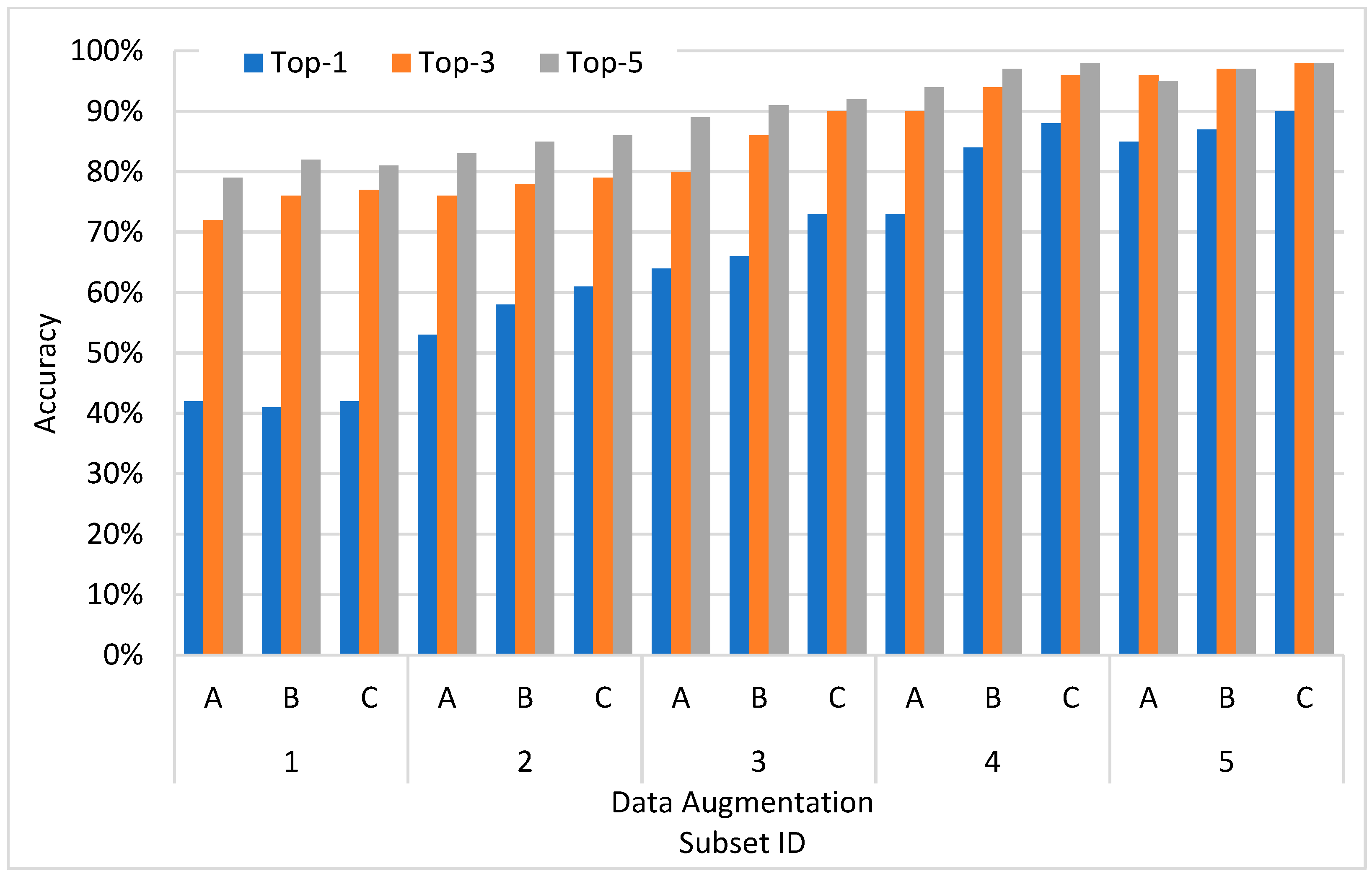
• It is important to select the right data augmentation. Appropriate data augmentation can help models to better learn sample features and reduce the overfitting problems caused by small datasets. Basic data augmentation should be adopted when new learning is adopted. When the model has no pre-training “knowledge”, an excessively complicated input interference prevents the models from learning basic features; when a combination of transfer learning + fine-tuning is adopted, it is recommended to use more complicated data enhancement (such as CutMix). If the model has pre-trained “knowledge”, strong input interference can help the models learn deep features;
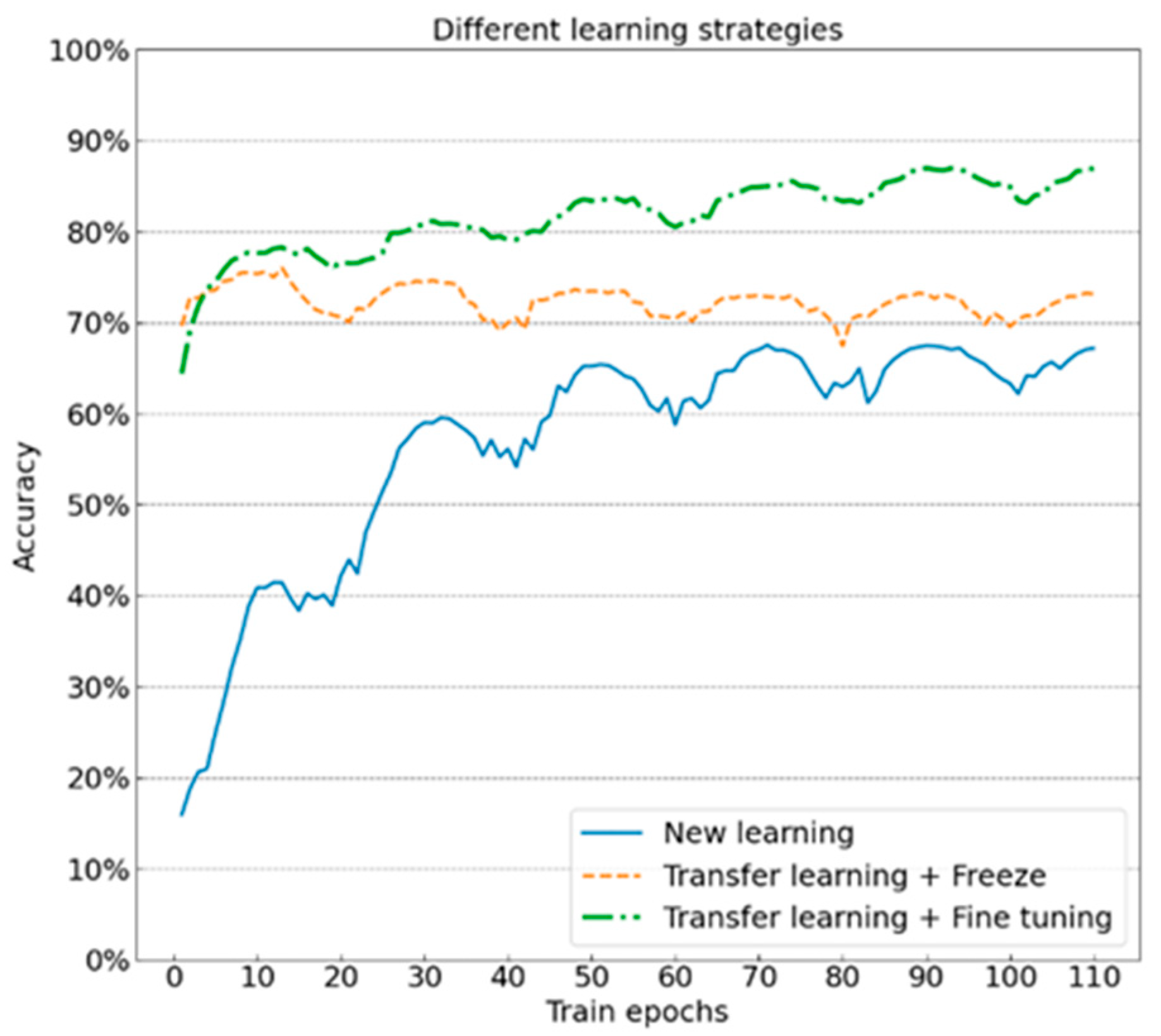
• Transfer learning can help models learn generically featured “knowledge” from other datasets. Learning the target dataset based on this “knowledge” can greatly improve the model performance. The training time needed for the model to achieve the same classification accuracy is greatly reduced, and the average classification accuracy is improved by 10~20% compared to the new learning model;
• The ability of transfer learning can be better exerted with fine-adjusting pre-training parameters than freezing pre-training parameters. Although the parameters of feature extraction in the transfer model are very close to the optimal solution, the fine-tuning is needed on this basis due to the differences between the datasets. According to the experimental results, the effect of the transfer learning model with fine-tuning or freezing is better than that of new learning, while the effect of the combination of transfer learning + fine-tuning is improved by 8% on average compared to the combination of transfer learning + freezing.

References

- Estruch, J.J.; Carozzi, N.B.; Desai, N.; Duck, N.B.; Warren, G.W.; Koziel, M.G. Transgenic Plants: An Emerging Approach to Pest Control. Nat. Biotechnol. 1997, 15, 137–141. [Google Scholar] [CrossRef] [PubMed]
- Faithpraise, F.; Birch, P.; Young, R.; Obu, J.; Faithpraise, B.; Chatwin, C. Automatic Plant Pest Detection & Recognition Using K-Means Clustering Algorithm & Correspondence Filters. Int. J. Adv. Biotechnol. Res. 2013, 4, 1052–1062. [Google Scholar]
- Samanta, R.K.; Ghosh, I. Tea Insect Pests Classification Based on Artificial Neural Networks. Int. J. Comput. Eng. Sci. 2012, 2, 1–13. [Google Scholar]
- Al-Hiary, H.; Bani-Ahmad, S.; Reyalat, M.; Braik, M.; Alrahamneh, Z. Fast and Accurate Detection and Classification of Plant Diseases. Int. J. Comput. Appl. 2011, 17, 31–38. [Google Scholar] [CrossRef]
- Dyrmann, M.; Karstoft, H.; Midtiby, H.S. Plant Species Classification Using Deep Convolutional Neural Network. Biosyst. Eng. 2016, 151, 72–80. [Google Scholar] [CrossRef]
- Krizhevsky, A.; Sutskever, I.; Hinton, G.E. ImageNet Classification with Deep Convolutional Neural Networks. In Advances in Neural Information Processing Systems; Curran Associates, Inc.: Lake Tahoe, NV, USA, 2012; Volume 25. [Google Scholar]
- Ning, X.; Duan, P.; Li, W.; Zhang, S. Real-Time 3D Face Alignment Using an Encoder-Decoder Network with an Efficient Deconvolution Layer. IEEE Signal Processing Lett. 2020, 27, 1944–1948. [Google Scholar] [CrossRef]
- CVPR 2017 Open Access Repository. Available online: https://openaccess.thecvf.com/content_cvpr_2017/html/Huang_Densely_Connected_Convolutional_CVPR_2017_paper.html (accessed on 24 March 2022).
- Atlam, M.; Torkey, H.; El-Fishawy, N.; Salem, H. Coronavirus Disease 2019 (COVID-19): Survival Analysis Using Deep Learning and Cox Regression Model. Pattern Anal. Appl. 2021, 24, 993–1005. [Google Scholar] [CrossRef] [PubMed]
- Salem, H.; Attiya, G.; El-Fishawy, N. Gene Expression Profiles Based Human Cancer Diseases Classification. In Proceedings of the 2015 11th International Computer Engineering Conference (ICENCO), Cairo, Egypt, 29–30 December 2015; pp. 181–187. [Google Scholar]
- Deep Learning|Nature. Available online: https://www.nature.com/articles/nature14539 (accessed on 24 March 2022).
- Ren, S.; He, K.; Girshick, R.; Sun, J. Faster R-CNN: Towards Real-Time Object Detection with Region Proposal Networks. In Advances in Neural Information Processing Systems; Curran Associates, Inc.: Montréal, QC, Canada, 2015; Volume 28. [Google Scholar]
- Shelhamer, E.; Long, J.; Darrell, T. Fully Convolutional Networks for Semantic Segmentation. IEEE Trans. Pattern Anal. Mach. Intell. 2017, 39, 640–651. [Google Scholar] [CrossRef] [PubMed]
- Reyes, A.K.; Caicedo, J.C.; Camargo, J.E. Fine-Tuning Deep Convolutional Networks for Plant Recognition. CLEF 2015, 1391, 467–475. [Google Scholar]
- Zhang, H.; He, G.; Peng, J.; Kuang, Z.; Fan, J. Deep Learning of Path-Based Tree Classifiers for Large-Scale Plant Species Identification. In Proceedings of the 2018 IEEE Conference on Multimedia Information Processing and Retrieval (MIPR), Miami, FL, USA, 10–12 April 2018; pp. 25–30. [Google Scholar]
- Wu, X.; Zhan, C.; Lai, Y.-K.; Cheng, M.-M.; Yang, J. IP102: A Large-Scale Benchmark Dataset for Insect Pest Recognition. In Proceedings of the 2019 IEEE/CVF Conference on Computer Vision and Pattern Recognition (CVPR), Long Beach, CA, USA, 15–20 June 2019; pp. 8779–8788. [Google Scholar]
- Xie, C.; Wang, R.; Zhang, J.; Chen, P.; Dong, W.; Li, R.; Chen, T.; Chen, H. Multi-Level Learning Features for Automatic Classification of Field Crop Pests. Comput. Electron. Agric. 2018, 152, 233–241. [Google Scholar] [CrossRef]
- Ayan, E.; Erbay, H.; Varçın, F. Crop Pest Classification with a Genetic Algorithm-Based Weighted Ensemble of Deep Convolutional Neural Networks. Comput. Electron. Agric. 2020, 179, 105809. [Google Scholar] [CrossRef]
- Nanni, L.; Maguolo, G.; Pancino, F. Insect Pest Image Detection and Recognition Based on Bio-Inspired Methods. Ecol. Inform. 2020, 57, 101089. [Google Scholar] [CrossRef] [Green Version]
- Kingma, D.P.; Ba, J. Adam: A Method for Stochastic Optimization. arXiv 2017, arXiv:1412.6980. [Google Scholar]
- Deng, L.; Wang, Y.; Han, Z.; Yu, R. Research on Insect Pest Image Detection and Recognition Based on Bio-Inspired Methods. Biosyst. Eng. 2018, 169, 139–148. [Google Scholar] [CrossRef]
- Bollis, E.; Pedrini, H.; Avila, S. Weakly Supervised Learning Guided by Activation Mapping Applied to a Novel Citrus Pest Benchmark. In Proceedings of the 2020 IEEE/CVF Conference on Computer Vision and Pattern Recognition Workshops (CVPRW), Seattle, WA, USA, 14–19 June 2020; pp. 310–319. [Google Scholar]
- Ren, F.; Liu, W.; Wu, G. Feature Reuse Residual Networks for Insect Pest Recognition. IEEE Access 2019, 7, 122758–122768. [Google Scholar] [CrossRef]
- Kasinathan, T. Insect Classification and Detection in Field Crops Using Modern Machine Learning Techniques. Inf. Process. Agric. 2021, 12, 446–457. [Google Scholar] [CrossRef]
- Thenmozhi, K.; Srinivasulu Reddy, U. Crop Pest Classification Based on Deep Convolutional Neural Network and Transfer Learning. Comput. Electron. Agric. 2019, 164, 104906. [Google Scholar] [CrossRef]
- Ung, H.T.; Ung, H.Q.; Nguyen, B.T. An Efficient Insect Pest Classification Using Multiple Convolutional Neural Network Based Models. arXiv 2021, arXiv:2107.12189. [Google Scholar]
- Khan, M.K.; Ullah, M.O. Deep Transfer Learning Inspired Automatic Insect Pest Recognition. In Proceedings of the 3rd International Conference on Computational Sciences and Technologies; Mehran University of Engineering and Technology, Jamshoro, Pakistan, 17–19 February 2022; Volume 8. [Google Scholar]
- Nanni, L. High Performing Ensemble of Convolutional Neural Networks for Insect Pest Image Detection. Ecol. Inform. 2022, 67, 101515. [Google Scholar] [CrossRef]
- Yang, X.; Luo, Y.; Li, M.; Yang, Z.; Sun, C.; Li, W. Recognizing Pests in Field-Based Images by Combining Spatial and Channel Attention Mechanism. IEEE Access 2021, 9, 162448–162458. [Google Scholar] [CrossRef]
- He, K.; Zhang, X.; Ren, S.; Sun, J. Deep Residual Learning for Image Recognition. arXiv 2015, arXiv:1512.03385. [Google Scholar]
- Xie, S.; Girshick, R.; Dollár, P.; Tu, Z.; He, K. Aggregated Residual Transformations for Deep Neural Networks. arXiv 2017, arXiv:1611.05431. [Google Scholar]
- Szegedy, C.; Vanhoucke, V.; Ioffe, S.; Shlens, J.; Wojna, Z. Rethinking the Inception Architecture for Computer Vision. arXiv 2015, arXiv:1512.00567. [Google Scholar]
- Simonyan, K.; Zisserman, A. Very Deep Convolutional Networks for Large-Scale Image Recognition. arXiv 2015, arXiv:1409.1556. [Google Scholar]
- El-Shafai, W.; Almomani, I.; AlKhayer, A. Visualized Malware Multi-Classification Framework Using Fine-Tuned CNN-Based Transfer Learning Models. Appl. Sci. 2021, 11, 6446. [Google Scholar] [CrossRef]
- Yun, S.; Han, D.; Oh, S.J.; Chun, S.; Choe, J.; Yoo, Y. CutMix: Regularization Strategy to Train Strong Classifiers with Localizable Features. arXiv 2019, arXiv:1905.04899. [Google Scholar]
- Duchi, J.; Hazan, E.; Singer, Y. Adaptive Subgradient Methods for Online Learning and Stochastic Optimization. J. Mach. Learn. Res. 2011, 12, 2121–2159. [Google Scholar]