Linear and Non-Linear Population Retrieval with Femtosecond Optical Pumping of Molecular Crystals for the Generalised Uniaxial and Biaxial Systems

Abstract

Femtosecond optical measurements of photoexcitable molecular crystals carry ultrafast dynamics information with structural sensitivity. The creation and detection of transient dynamics depend on the optical parameters, as well as the explicit molecular structure, crystal symmetry, crystal orientation, polarisation of the photoexciting beam, and interaction geometry. In order to retrieve the linear and non-linear population transfer in photoexcited crystals, excitation theory is combined here with the calculation of birefringence decomposition and is shown for both the generalised uniaxial and biaxial systems. A computational tool was constructed based on this treatment to allow modelling of electric field decomposition, dipole projections, and non-linear excitation population levels. This is available open source and with a GUI for ease of use. Such work has applications in two areas of ultrafast science: multidimensional optical crystallography and femtosecond time-resolved X-ray crystallography.

1. Introduction

Molecular physics applications in ultrafast science are rapidly developing in multiple areas of spectroscopy and X-ray diffraction. Here, we consider the application of ultrafast techniques to single crystal studies, with the aim to interpret and exploit the structural sensitivity of the information obtained from photoinduced dynamics.

Practical approaches for quantitative analysis of ultrafast processes in crystals combine the areas of crystal optics, X-ray crystallography, and non-linear optical excitation theory. The basis for this approach is formed by the electric field decomposition in the presence of birefringence, and the resulting linear combination of the separate field-dipole interactions for the orthogonal modes that solve Maxwell’s equations in anisotropic media. In the area of ultrafast spectroscopy, two-dimensional electronic spectroscopy (2DES) is a powerful technique that provides ultrafast dynamics information [1,2]. The methodology, analysis, and theory of 2DES [3] is highly advanced and has shown many fascinating examples and results for complex materials, including photosynthesis [4,5], solid state physics, and solar cell science [6]. Two-dimensional electronic spectroscopy measurements intrinsically have ultrafast time resolution and can be applied to a multitude of molecular processes for isolated pigments, as well as structures and aggregates with weak or strong coupling. There are very similar considerations for two-dimensional infrared spectroscopy of oriented single crystals and other four-wave mixing techniques such as time-domain impulsive Raman spectroscopy. There are many different types of ultrafast and non-linear spectroscopy experiments. Experimentally, ultrafast spectroscopy typically uses femtosecond optical pulses that are resonant with electronic and/or vibrational transitions and create and interrogate coherences and populations in molecular systems. Recently, the theoretical framework was shown for two-dimensional spectroscopy measurements of oriented single crystals [7]. This is a unique application, where the non-linear spectroscopy measurement is sensitive to explicit molecular structure, crystal symmetry, crystal orientation, and polarisation of the incident field. The third-order response of molecular crystals is generally different from that of isotropic solutions. Depending on the crystal symmetry, the interesting case arises where selected Feynman pathways that contribute to the overall third-order response become symmetry-disallowed, whereas the allowed pathways are weighted via the symmetry progressions of the four-point correlation functions for each individual coherence. An analytical calculation of the resulting four-point correlation functions was shown, from the initial result of using crystal classes or reduced point-group symmetries, to include all point-group symmetries following definition of additional zero-valued tensor elements [7]. The method therefore adheres to Neumann’s Principle, which states that the symmetry elements of any physical property of a crystal must include the symmetry elements of the point group of the crystal [8]. The theory was shown and demonstrated for selected polarisation conditions that correspond to the principal directions of refractive indices. Here, we provide a set of tools to model the electric field decomposition and associated dipole projections in a more generalised approach to extend such measurements to include all crystal orientations and polarisation directions, excluding the isotropic directions of the optic axes.

We emphasise that serial femtosecond crystallography (SFX), which is an emerging technique at X-ray free-electron laser facilities (XFELs) [9,10,11], could benefit from the consideration of this orientation-sensitive information that arises from crystal photoexcitation. Using pump-probe techniques, femtosecond time resolution has been achieved for X-ray crystallography of macromolecules. The SFX approach relies on collecting many stationary diffraction images of micrometre-sized crystals in a distribution of random orientations. Typically, many thousands of individual crystals are measured. Scaling and merging techniques then find the magnitudes of the structure-factor amplitudes that are used for structure solution. Importantly, this analysis is also generally applied to time-resolved, pump-probe SFX data. The different crystal orientations, however, result in differences of linear and non-linear population dynamics, such that the usual methodology, which averages over all orientations, loses this information that is intrinsically present in the dataset. Furthermore, averaging suppresses the light-induced differences relative to orientations that maximise the interactions. Such phenomenon can be particularly relevant for low quantum yield (<10%) reactions where the signal to noise ratio is a significant issue. Another observation is that, since SFX datasets already contain orientational information for each indexed frame, the methodology we propose can be retroactively applied to previously collected datasets.

A general method has previously been proposed for the calculation of populations from photoexcitation in oriented uniaxial crystals (which include trigonal, tetragonal, and hexagonal point-group symmetries) [12]. Here, we extend the analysis to include biaxial crystals and provide practical methods and a set of tools for decomposing the electric field of the pump laser and calculating the associated modified dipole projections. Furthermore, we provide practical guidance and methods to deal with crystal orientation, indicatrix determination, indexing, and molecular structure transforms, as well as solving ambiguities where these arise. We go on to describe and present a computational toolbox that combines birefringence decomposition and calculation with non-linear excitation theory. The toolbox is presented for the purpose that it can be applied to specific examples and systems in two-dimensional optical crystallography and in TR-SFX. The toolbox is provided as open source and is user friendly, including a graphical user interface and worked examples.

2. Crystal Orientation and Practical Determination of Principal Indices of Refraction

The following provides a summary and practical guidance to determine crystal orientation, as well as how the measurement and determination of the directions and values for the principal indices of refraction can be carried out. This is necessary since the methods for calculation of population transfer in Section 4 and Section 6 will be presented in this coordinate frame. In order to add the molecular dynamics modelling, the crystallographic axes must be rotated onto the optical frame. Most of the following information is available in standard texts of crystallography and mineralogy such as Nye (1959) [8]. However, methods commonly used in mineralogy are rarely used in protein crystallography or chemical crystallography and are worth summarising for these specific purposes.

Firstly, we summarise the crystal classes with respect to the directions of principal indices of refraction. These can be represented by the optical indicatrix. This three-dimensional ellipsoid is given by the following:

$$\frac{x^2}{n_1^2}+\frac{y^2}{n_2^2}+\frac{z^2}{n_3^2}=1$$

(1)

where $n_1$, $n_2$, and $n_3$ are the principal refractive indices of the crystal.

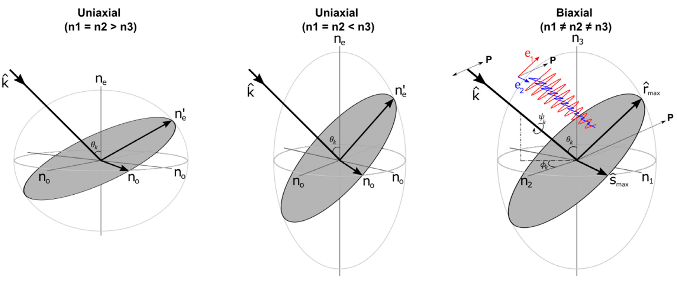
2.1. Uniaxial Crystals

For uniaxial crystals, $n_1=n_2$ and the optical indicatrix is rotationally symmetric about the optic axis. The optic axis here corresponds to the direction of the high-symmetry crystallographic axis. A ray travelling along this direction in the crystal encounters an isotropic medium and double diffraction does not occur. Uniaxial crystals have two principal axes of refraction and magnitudes of refractive index associated with them. For trigonal, tetragonal, and hexagonal point-group symmetries, the index ellipsoid is always rotationally symmetric. The consequence is that the decomposition of polarised radiation by double refraction only depends on the angle between the ray direction and the optic axis. When the polarisation direction is along one of the two principal axes of refraction, no double refraction occurs, given that the component in the other direction is zero. For an incident k-vector, the intersection plane between the normal of the k-vector and the indicatrix of a uniaxial crystal produces an ellipse (Figure 1 left & middle). The semi-axes of this ellipse correspond to the orthogonal radiation modes that solve Maxwell’s equations for anisotropic media. Thus, for any k-vector direction the polarisation direction of these modes is invariant and the initial polarisation of the incident wave is decomposed along these modes and determines their amplitudes accordingly. This treatment disregards attenuation, which will result in a circular polarisation. For many practical examples, attenuation is limited and this approximation can be made. In practice, micrometre-sized protein crystals have relatively low absorption values (<0.3 OD) due to the large unit cell that contains only a single or a few chromophores. If larger crystals are studied, the measurement of dichroic absorption along the principal axis will allow a straightforward modification of the birefringence decomposition for low attenuation to allow for circular polarisation conditions. For crystals of small molecules, the optical density is much larger and optical penetration may be insufficient, even to allow transmission measurements. Reflection measurements are more appropriate for such materials. Similarly, optical activity is disregarded but would have only a very small effect on the indicatrix. Although in isolated cases optical activity could modify the directions of decomposition, this is rare and possible only if the index differences in the absence of a field are very close in magnitude. Consequently, optical activity is also neglected in the following description. Therefore, explicit measurements of the magnitude of the indices of refraction and of the intrinsic birefringence are not necessary for uniaxial symmetries for the purpose of analysis of linear and non-linear population dynamics.

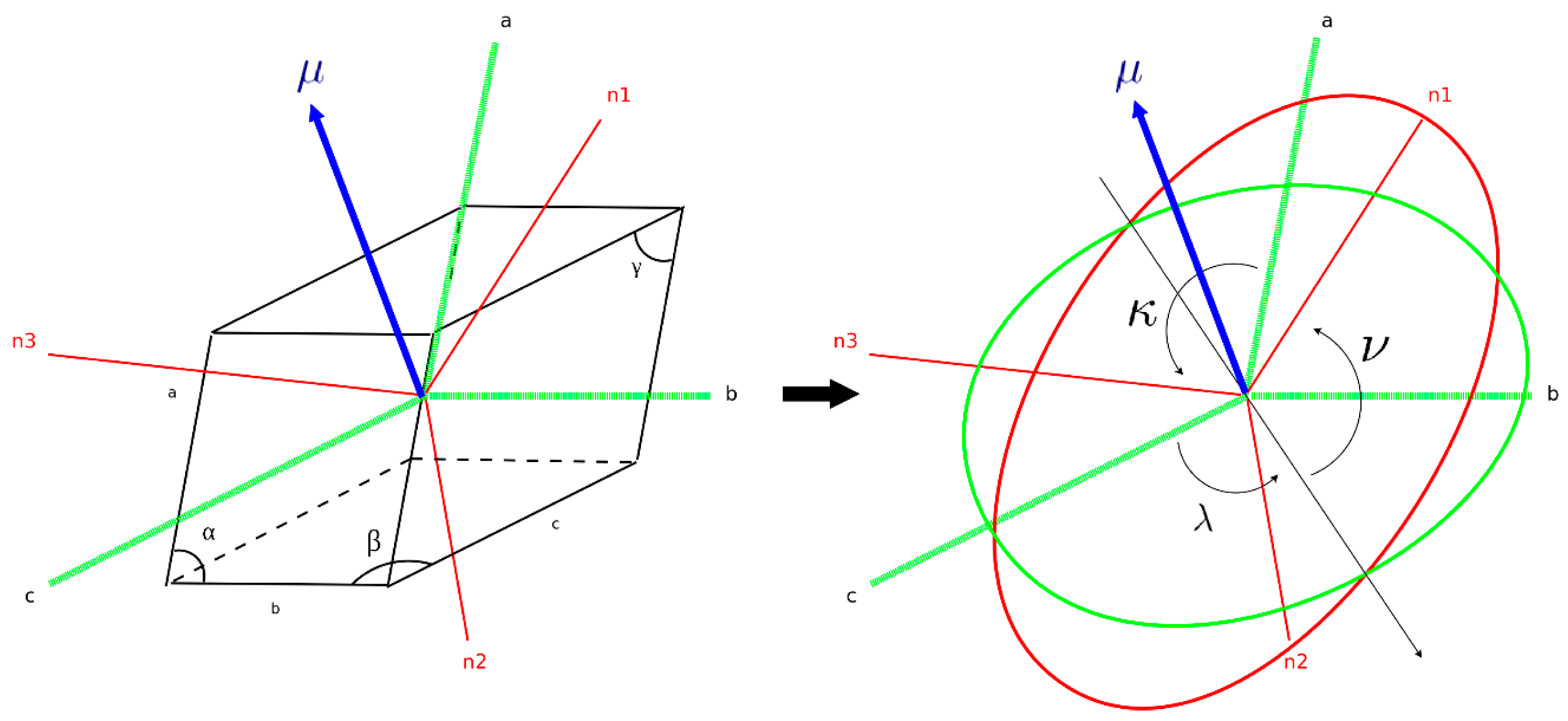
2.2. Biaxial Crystals

For biaxial symmetries, it is necessary to obtain values for all three principal refractive indices (Figure 1), in addition to a determination of their directions in the crystallographic frame, depending on the presence or absence of two-fold symmetry elements in their point group. Triclinic, monoclinic, and orthorhombic symmetries belong to the crystal classes that are biaxial, where $n_1\ne n_2\ne n_3$. In triclinic crystals, the absence of symmetry elements causes there to be no relation between the directions of the principal refractive indices and the crystallographic directions, other than by coincidence [7,8,13,14]. In order to measure and obtain this relationship, it is necessary to combine birefringence measurements in the polarising microscope together with an indexing determination for the crystal morphology. Starting with the latter, measurements of the angles between crystal faces using the microscope and an appropriate three-axis rotation stage can result in unambiguous indexing for selected or all crystal faces. The unit cell dimensions must be determined by X-ray crystallographic indexing using rotation ranges. This approach will be facilitated if crystal faces include singular indices rather than higher order indices. This condition is met for many protein crystals [15]. If indexing by visual means fails, it will be necessary to perform a face-indexing using X-ray crystallography, which provides the orientation matrix for the correct indexing solution. Monoclinic crystals include one two-fold symmetry axis, which by convention is the b-axis. The two-fold symmetry ensures that one of the principle refractive index axes is in the direction of the crystallographic b-axis. The consequence is that, for a k-vector perpendicular to the b-axis, double refraction occurs such that one polarisation direction corresponds to the b-axis and is furthermore wavelength-independent. For any other k-vector, knowledge of the directions of n₁ and n₃ an8tals, each axis is associated with a two-fold symmetry operation which fixes the directions of the principle refractive indices in the crystallographic directions. Indexing of orthorhombic crystals may present particular challenges. The unit cell is rectangular, and crystals may either appear rectangular or show more facets (e.g., they can have a dodecahedral shape). The visual measurement under the microscope of the interfacial angles, together with the unit cell dimension information, can usually allow indexing in this manner [15]. When crystal morphology is rectangular, or appears rectangular in at least four directions, the crystal faces can either reflect the orientation of the unit cell or they are combination directions. As an example, Perutz showed that orthorhombic crystals of carboxy-haemoglobin appear almost square in cross section, but end in bipyramidal prisms with {1 1 1} faces. The faces for the central part with a square cross section are {1 1 0} [16]. The direction of the principal refractive indices can therefore be determined; however, there can arise an ambiguity for assignment of index to those directions. Typically, X-ray crystallographic face indexing is needed. In general, for biaxial crystals it is necessary to make measurements of the magnitude of all three refractive indices $n_1$, $n_2$, and $n_3$ and of the intrinsic birefringence values.

In order to make measurements of the magnitude of birefringence, it is first necessary to orient crystals according to a known index. Crystals must also be embedded in mother liquor such that refraction at the surface is minimised. Mounting in quartz capillaries can aid in this part. When birefringent crystals are viewed under crossed polarisers, two situations can result in extinction. Either the view is along one of the two optic axes (in which case the crystal appears to be optically isotropic) or one of the principal axes of refractive index is aligned with a polariser direction. Consequently, under these conditions, the crystals will appear bright under parallel polarisers. When a crystal is rotated to the extinction point, all colours vanish and the view appears dark. To measure the difference in refractive index between principal axes, the crystal is rotated 45° away from the extinction point and a Berek compensator is inserted in the light path between the polarisers.

The retardance $\left(R\right)$ between two waves is the product of the birefringence ($\mathsf{\Delta }n)$ and the optical path length through the crystal (d) and must also be measured:

$$R=∆n\times d$$

(2)

The retardance is also given as a function of the wavelength ${\lambda }_0$ and the phase difference $\varphi$ between the waves:

$$R=\left(\varphi \times {\lambda }_0\right)/2$$

(3)

The fast axis of the Berek compensator should be along the slow axis of the crystal in order to arrive at a measurement of compensation of retardance. The compensator is calibrated such that the retardance value can be read after rotation of the drum, once the extinction point is obtained. The $\mathsf{\Delta }{n}_{a,b,c}$ values measured in the a, b and c directions should be measured individually. In addition, these values are related according to:

$$\mathsf{\Delta }{n}_a=\mathsf{\Delta }{n}_b-\mathsf{\Delta }{n}_c$$

(4)

where $\mathsf{\Delta }{n}_a=n_c-n_b, \mathsf{\Delta }{n}_b=n_c-n_a, \mathsf{\Delta }{n}_c=n_b-n_a,$ if $\mathsf{\Delta }{n}_a$ is the smallest birefringence and $\mathsf{\Delta }{n}_b$ is the largest birefringence. This relationship allows the verification of the independent intrinsic birefringence measurements.

The values of birefringence of crystals are typically in the range of 10⁻²–10⁻⁴ [15]. An alternative to the Berek compensator measurement uses the conventional Michel-Levy chart [17]. The method is less precise and only provides an estimate. In addition, since Newton’s series appear in multiple orders, there may be uncertainty in the order of assignment. Using either visual colour determination or a spectrometer measurement, there may also be significant error in the estimate of birefringence determination using this method. In optical mineralogy, the phase contrast (or oblique illumination) method would additionally provide a means for estimating the refractive indices, but this requires immersion in liquids with a large refractive index [18].

An additional method that is used in optical mineralogy that may be useful for certain cases of resolving indexing ambiguity is conoscopy analysis. Conoscopy is the examination of the interference figures and colour patterns in the focal plane of the microscope objective lens, produced by an anisotropic crystalline section viewed under convergent light illumination and crossed polarisers. This method requires the use of a Bertrand lens or phase telescope, or alternatively, a conoscope lens that is used in the polarising microscope. The method may be less suitable for protein crystals, as single crystals need to fill the field of view or they must be in an aperture to view the interference image. Conoscopy images are instructive when viewing either in the direction of an optic axis or perpendicular to an optic axis. The optics allow a two-dimensional projection and view of the interference pattern and colours. Conoscopy can directly distinguish uniaxial and biaxial crystals. The use of waveplates and quarter waveplates allow the identification of negative and positive crystals, hence aiding in the assignment of fast and slow crystal axes [19]. For biaxial crystals, conoscopy can also show the angle between the two optic axes, which is an independent verification of the indicatrix modelling following the index determination.

In order to construct the indicatrix, the absolute values of the principle refractive indices should be determined. The mean refractive index $\langle n\rangle$ can be derived from the value of the index increment $\delta n/\delta c$ for a different concentration in solution, in combination with the calculated concentration in the crystal from the unit cell dimension.

$$\langle n\rangle =n_{solvent}+\left(\frac{\delta n_{sample}}{\delta c}\right)\times c$$

(5)

For example, a value of index increment $\delta n/\delta c$ = 0.187 mL/g was measured at the wavelength of 436 nm by Holtzer et al. [20] for the protein tropomyosin.

2.3. Cubic Crystals

Finally, we briefly consider cubic crystals. Crystals with point-group groups 432, $\overline{4}$3m, 23, m3, or m3m are not doubly refracting and also appear isotropic in the linear optical response. However, the non-linear optical response of cubic crystals does not equal that of isotropic solutions and samples. Specifically, isotropic materials have 21 non-zero third-order susceptibility tensor elements, of which only 3 are independent. Isotropic materials have 60 zero-valued third-order tensor elements in the dipole approximation [21]. All cubic point groups also show 21 non-zero tensor elements; however, 7 of those are independent for 23 and m3 point groups, and 4 are independent for 432, $\overline{4}$3m, and m3m point groups. As an example, the isotropic tensor element ${\chi }_{yyzz}$ also equals ${\chi }_{zzyy}$, whereas for point groups 23 and m3 it does not; rather, ${\chi }_{yyzz}$ also equals ${\chi }_{zzxx}$ and ${\chi }_{xxyy}$. Then, for point groups 432, $\overline{4}$3m, and m3m, ${\chi }_{yzyz}$ is equal to the same elements as those in isotropic materials, but the independent group ${\chi }_{xxxx}={\chi }_{yyyy}={\chi }_{zzzz}$ appears which does not follow the isotropic sum rule ${\chi }_{xxxx}={\chi }_{xxyy}+{\chi }_{xyxy}+{\chi }_{xyyx}$. Therefore, non-linear behaviour of cubic crystals is distinct from isotropic solutions. The non-linear optical response for crystal symmetries has been discussed previously and is more appropriately quantified in terms of the response-function formalism [7]. This is beyond the scope of this paper. The objective here is to generalise the use of non-linear cross sections in combination with birefringence decomposition.

3. Rotation Matrix for Transition Dipole Moment to the Optical Frame

The objective of this contribution is to compute the linear and non-linear population transfer following birefringence decomposition of an arbitrary k-vector, with an emphasis on showing its application to the more challenging biaxial symmetries. The combination of crystal optics that evaluate birefringence decomposition in the explicit molecular frame and non-linear excitation theory is the key technique for analysis and is explicitly shown for biaxial crystals for the first time here. The X-ray crystallographic coordinates from the structure solution are needed as the first step in the analysis. Typically, quantum chemical calculations of transition dipole moments are conducted in the molecular frame using quantum chemistry methods. Electronic transitions are often accurately found at the TD-DFT level using an appropriate density functional, such as CAM-B3LYP in the case of light atoms [22]. With Cartesian coordinates in the crystallographic directions, an Euler rotation matrix then transforms this direction to the optical frame [14] (Figure 2). In the following, all optical calculations are performed in the coordinate frame of the principal refractive indices.

4. Electric Field Decomposition Using the Indicatrix

The decomposition of the electric field in uniaxial and biaxial crystals has been previously described by Sage et al. [14] and others [13].

In a uniaxial crystal, due to symmetry, the refractive index in two of the crystal axes is equal ($n_1=n_2 \ne n_3$). This results in the field decomposing into an ordinary ($e_o$) and extraordinary ($e_e$) optic axis, where the refractive index of the ordinary is $n_{e_o}=n_1=n_2$, whereas that of the extraordinary depends on the angle of the incident ray vector ($\widehat{k}$) and the high-symmetry axis ${\theta }_k$, such that $n_{e_e}=n_3\cos {\theta }_k$. As previously stated, this is true except in the special case of ${\theta }_k\to 0$, where $\widehat{k}$ is aligned down the optic (high-symmetry) axis and the crystal appears isotropic.

In a biaxial crystal ($n_1\ne n_2\ne n_3$), the decomposed electric field vectors are determined by the extrema of the ellipse that bisects the indicatrix ellipsoid in the plane normal to $\widehat{k}$ (Figure 1 right). In our model, we determine these vectors numerically for each $\widehat{k}$ or crystal orientation. A random vector is generated perpendicular to $\widehat{k}$, ($\widehat{r}$) and normalized, and the cross product of the two is used to find the third corresponding perpendicular vector ($\widehat{s}$). Then, $\widehat{r}$ and $\widehat{s}$ are iteratively rotated about $\widehat{k}$ (i.e., in the plane of the ellipse as shown in Figure 1) until the maxima solutions of Equation (1) are found (those being the semi-major axes of the ellipse). It is important to note that this method requires the condition that $n_3>n_1 \& n_2$. Figure 3 shows the calculation of the intrinsic birefringence by computing the difference between the refractive index of the two decomposed vectors as a function of orientation such than minima represent points where the axis are equal and hence the location of the optic axes. This was performed for two test case crystals using the literature values of refractive index for topaz and muscovite, in can be seen how the relative distribution of the refractive indices determines the position of the optic axes.

5. Dipole Projections

From Sage et al. [14] the absorption in a particular direction for a biaxial crystal is given as:

$$A={\displaystyle \sum }_{\alpha }3{ϵ}_{\alpha }cd\frac{1}{m}{\displaystyle \sum }_{j=1}^m{\left({\widehat{\mu }}_{\alpha j}·\widehat{e}\right)}^2$$

(6)

In orthorhombic space groups, the two-fold symmetry in all three principal directions results in the coincidence of the principal optic axes being with the crystal axes, and also the value of ${\left({\widehat{\mu }}_{\alpha j}·\widehat{e}\right)}^2$ being invariant in the two-fold rotation such that the transition dipole orientations can be described with respect to the crystallographic axes [14]:

$${\widehat{\mu }}_{\alpha j}=\left(\sin {\theta }_{\alpha j}\cos {\varphi }_{\alpha j},\sin {\theta }_{\alpha j}\sin {\varphi }_{\alpha j},\cos {\theta }_{\alpha j}\right)$$

(7)

where $\theta$ and $\varphi$ are the polar and azimuthal angles, measured with respect to the chosen crystal axis. In monoclinic space groups there is only one two-fold symmetry direction that results in the alignment of one optic axis with the crystallographic b-axis. However, in triclinic space groups the absence of symmetry elements causes there to be no relationship between the crystallographic and optical directions. Therefore, we present the treatment for biaxial crystals only in relationship to the optical directions. In this work, we define these angles with respect to the high refractive index axis (Figure 1 right). This results in the dipole projection being simply the square projection of these two vectors summed over all dipoles within the asymmetric unit, $\langle {\left(\widehat{\mu }·\widehat{e}\right)}^2\rangle$.

In the uniaxial case, the value of ${\langle \left(\widehat{\mu }·\widehat{e}\right)}^2\rangle$ is strongly impacted by the rotational symmetry of the system [12,14], resulting in:

$${\langle \left(\widehat{\mu }·{\widehat{e}}_3\right)}^2\rangle ={\cos }^2{\theta }_d$$

(8)

$${\langle \left(\widehat{\mu }·{\widehat{e}}_1\right)}^2\rangle ={\langle \left(\widehat{\mu }·{\widehat{e}}_2\right)}^2\rangle =½\sin {\theta }_d$$

(9)

where ${\widehat{e}}_3$ is the high-symmetry axis. Combining (8) & (9) with $\widehat{k}$ in spherical coordinates gives the total value:

$${\langle \left(\widehat{\mu }·\widehat{e}\right)}^2\rangle =\left[co{s}^2{\theta }_k{\cos }^2{\mathsf{\theta }}_{\mathrm{d}},{\sin }^2{\theta }_k½{\sin }^2{\theta }_d, ½\sin {\theta }_d\right]\left[\begin{array}{c}x\\ y\\ z\end{array}\right]$$

(10)

The first observation is that this value is invariant in ${\varphi }_d$. Secondly, when looking at the distributions over all values of $\widehat{k}$ (see Supplementary Materials and [12]) it can be seen that dipoles aligned parallel to the high-symmetry axis result in a larger variation of ${\langle \left(\widehat{\mu }·\widehat{e}\right)}^2\rangle$, with a significant number of orientations where the term is actually suppressed. Conversely, when the dipole is oriented perpendicular to the high-symmetry axis, the maximum value that ${\langle \left(\widehat{\mu }·\widehat{e}\right)}^2\rangle$ is suppressed by is a factor of 2, though it is also noted that non-zero values are obtained over a larger number of orientations [12].

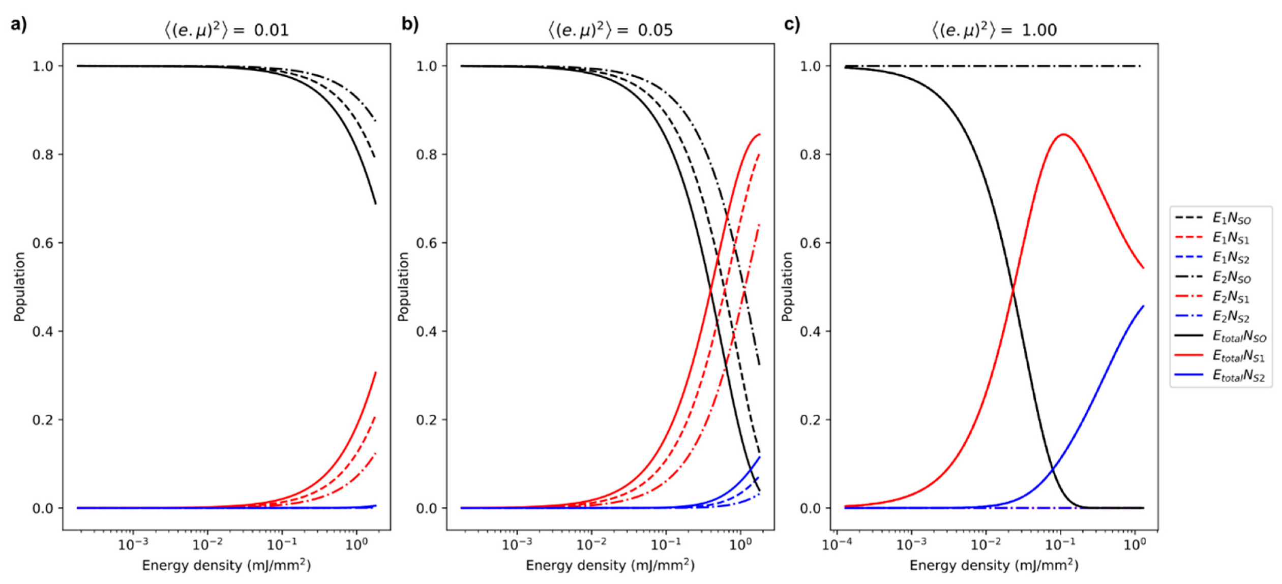
6. Linear and Non-Linear Excitation Calculations

Photoexcitation is modelled, as in Hutchison et al. [12], with a three-level system of ground-($S_0$), first-($S_1$), and second-($S_2$) excited state. The populations are calculated using the following rate equations:

$$N_{S_0}\left(t\right)=N_{S_0}\left(-\infty \right)\exp \left[\frac{{\sigma }_{S_{0\to 1}}F\left(t\right)}{\hslash \omega }\right]$$

(11)

$$N_{S_1}\left(t+dt\right)=N_{S_0}\left(-\infty \right)\left(1-\exp \left[\frac{{\sigma }_{S_{0\to 1}}F\left(t\right)}{\hslash \omega }\right]\right)-N_{S_2}\left(t\right)$$

(12)

$$N_{S_2}\left(t\right)=N_{S_1}\left(t\right)\left(1-\exp \left[\frac{{\sigma }_{S_{1\to 2}}F\left(t\right)}{\hslash \omega }\right]\right)$$

(13)

where $N_{S_n}$ is the population of the $S_n$ state, $N_{S_0}\left(-\infty \right)$ is the ground-state population calculated from the absorption, ${ϵ}_{S_0}$. ${\sigma }_n$ is the cross section of that state transition, and $F\left(t\right)$ and $\omega$ are the temporally integrated flux and central frequency of the excitation pulse, respectively. To incorporate the effect of the electric field decomposition, the pulse energy of each optic axis ($E_{e_n}$) is scaled by the dot product of that axis with the polarisation vector. The dipole projections are used to scale ${\sigma }_n$ such that ${\sigma }_{n}F\left(t\right)$ can be written as [12]:

$${\sigma }_{n}F\left(t\right)=\left[{\langle \left(\widehat{\mu }·{\widehat{e}}_1\right)}^2\rangle ·3{\sigma }_I\right] · {\mathrm{F}}_{{\mathrm{e}}_1}\left(t\right)dt+\left[{\langle \left(\widehat{\mu }·{\widehat{e}}_2\right)}^2\rangle ·3{\sigma }_I\right]·F_{e_2}\left(t\right)$$

(14)

where ${\langle \left(\widehat{\mu }·\widehat{e}\right)}^2\rangle$ is the total averaged dipole projection in the ${\widehat{e}}_n$ optic axis and ${\sigma }_I$ is the averaged isotropic cross section, as determined by spectroscopy on a solution or randomly oriented crystalline samples. An example of this calculation performed on a single orientation for several different pulse energies and values of ${\langle \left(\widehat{\mu }·\widehat{e}\right)}^2\rangle$ is shown in Figure 4.

7. Toolkit Program

A computational toolbox was constructed to allow the straightforward modelling of the electric field decomposition, associated dipole projections, and linear and non-linear optical excitation in uniaxial and biaxial crystals. It was constructed in python3 using the Anaconda [24] libraries and includes a graphically user interface (GUI) for ease of use. The code is open source and available at https://github.com/cdmhutchison/Xtal-orientation-excitation (accessed on 22 April 2022).

It consists of two main functions:

The first uses the theory described in Section 3 and Section 4. For a given (i) crystal type (uniaxial or biaxial), (ii) principal refractive indices, and (iii) dipole orientations, the code scans $\widehat{k}$ over all polar (${\theta }_k$), azimuth (${\varphi }_k$), and roll (${\psi }_k$) angles and generates arrays of electric field decompositions and associated values of ${\langle \left(\widehat{\mu }·\widehat{e}\right)}^2\rangle$. Depending on which frame is being considered, ${\psi }_k$ can correspond to the rotation of the crystal or the polarisation of the incident field.

The second function takes electric field vectors and values of ${\langle \left(\widehat{\mu }·\widehat{e}\right)}^2\rangle$ and uses the molecular extinction coefficients ($ϵ$) for linear excitation (${ϵ}_{S_0\to S_1}$), sequential double excitation (${ϵ}_{S_1\to S_2}$), and nonlinear absorption (${ϵ}_{nl}$), along with the crystal optical density and excitation pulse parameters to calculate the populations after excitation as described in Section 5.

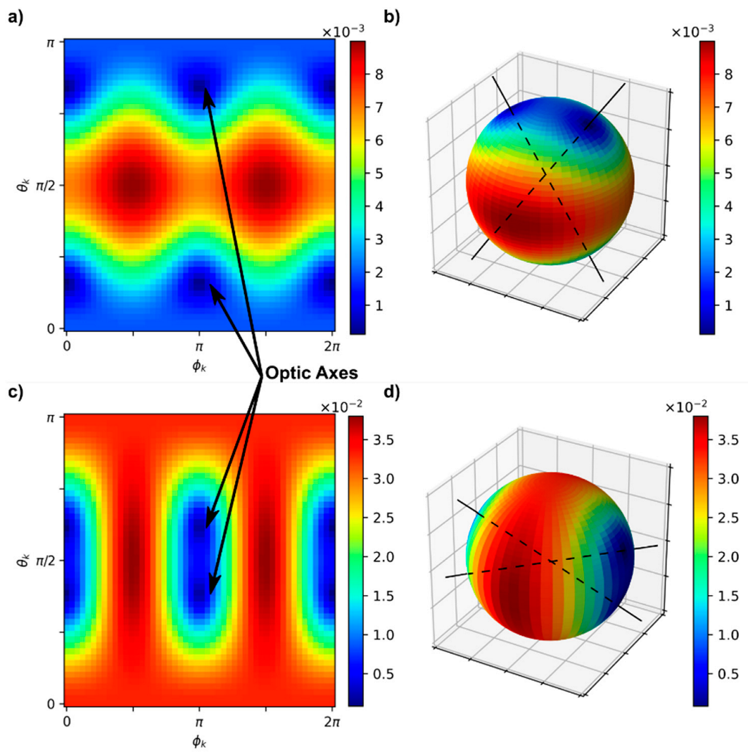
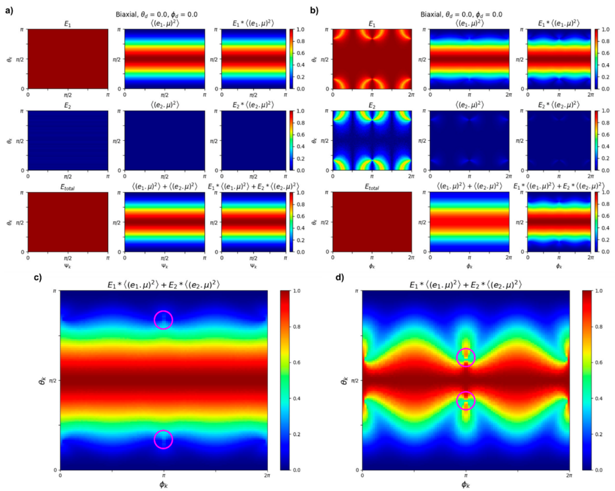
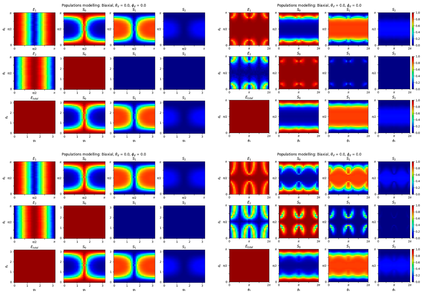
8. Biaxial Crystal Modelling Examples

Figure 5 shows modelled electric field and dipole projection distributions for two biaxial protein crystals with different refractive index distributions. A single dipole was included in the asymmetric unit aligned below the c-axis. In the first case (Figure 5a–c), the optic axis was aligned closer to the c-axis (Figure 3a,b); as such, the result was close to that of a uniaxial crystal with a dipole aligned to the high-symmetry axis. A large angular dependence was seen on ${\theta }_k$ with close to zero dependence on ${\psi }_k$. The biaxial birefringence manifested with a small dependence on ${\varphi }_k$, particularly near to the optic axis.

In the second case (Figure 5d & Supplementary Materials), the effect was far more pronounced as the optic axes are closer together and nearly perpendicular to the dipole projection. The result was a highly modified distribution of $E_1\ast {\langle \left(\widehat{\mu }·{\widehat{e}}_1\right)}^2\rangle +E_2\ast {\langle \left(\widehat{\mu }·{\widehat{e}}_2\right)}^2\rangle$.

Figure 6 shows the population calculation for the same two crystals described in Figure 3 and Figure 5. It can be seen that there is significant similarity between the shape of $E_n\ast {\langle \left(\widehat{\mu }·{\widehat{e}}_n\right)}^2\rangle$ and the relative pumping, with a significant excitation of $S_2$ population seen for some orientations and complete suppression for others for the same laser pulse parameters. This mapping could be used to sort an SFX dataset to distinguish between strongly- and weakly-pumped crystals.

9. Assumptions, Approximations, and Extensions of the Excitation Model

In order to keep the code as general as possible, and therefore, more applicable to the largest number of users/targets, we acknowledge that a number of simplifications were made. Firstly, the population modelling only considers the relative populations of three energy levels (ground-, single-, and double-excited states). In reality, the number of electronic states may be large and the dynamics of a system more complex, e.g. involving evolutions that can occur within the excitation pulse length. Stimulated emission pumping may be added if the carrier frequency, dynamic Stokes shift, and pulse duration support the process. Quantification of the stimulated-emission cross section can be conducted on the basis of modelling power density dependence of femtosecond transmission under such conditions [25]. Such modifications can be added in the provided toolbox by specifying the additional rate equations. Secondly, we make no assumptions about how the relative populations will evolve in the time between the excitation (pump) pulse and a potential measurement (probe), be that spectroscopic or diffraction-based. To tailor it to a specific scheme, the code could be simply modified to include more complex rate equations and further temporal evolution. The presented applications considered electronic excitation only. However, for low bandgap or spin transition systems, thermal excitation and lattice heating should be considered as well [26]. Finally, we do not consider the macroscopic crystal shape, such as the refraction that will occur at the crystal edges or any focusing that could occur with a curved-facet crystal (such as needles), both phenomena that will vary depending on exact crystal size and each’s orientation. For many applications, however, the refraction could be minimal if index matching of the solution or solvent is achieved.

10. Conclusions

This contribution shows methods and results that allow analysis of non-linear excitation for any direction of the incoming pulse and any crystal symmetry. The code and software toolbox that is provided can be directly used to apply the method for ultrafast measurements of single crystals, either for non-linear spectroscopy or X-ray crystallography. The polarisation dependence of four-wave mixing experiments is well known. Up to 81 non-zero third-order tensor elements can describe the total response, and they are tabulated in textbooks. A practical application that specifically selects a set of tensor elements for the analysis of the material response is typically conducted under conditions of precise alignment with one or more optic axes. Using the methods shown here, such experiments can also deal with other directions. As described in the introduction, there is also the additional application of serial crystallography. In this technique, a stream of small single crystals is used for pump-probe measurements. Although preferential crystal orientation in such jets is seen, usually there is a good coverage of all directions. Application of non-linear excitation theory using the method shown here is particularly useful in this case.

References

1. Mukamel, S. Multidimensional Femtosecond Correlation Spectroscopies of Electronic and Vibrational Excitations. Annu. Rev. Phys. Chem. 2000, 51, 691–729. [Google Scholar] [CrossRef] [PubMed] [Green Version]
2. Jonas, D.M. Two-Dimensional Femtosecond Spectroscopy. Annu. Rev. Phys. Chem. 2003, 54, 425–463. [Google Scholar] [CrossRef] [PubMed]
3. Jansen, T.L.C.; Saito, S.; Jeon, J.; Cho, M. Theory of coherent two-dimensional vibrational spectroscopy. J. Chem. Phys. 2019, 150, 100901. [Google Scholar] [CrossRef] [PubMed]
4. Tiwari, V.; Peters, W.K.; Jonas, D.M. Electronic resonance with anticorrelated pigment vibrations drives photosynthetic energy transfer outside the adiabatic framework. Proc. Natl. Acad. Sci. USA 2013, 110, 1203–1208. [Google Scholar] [CrossRef] [PubMed] [Green Version]
5. Chenu, A.; Scholes, G.D. Coherence in Energy Transfer and Photosynthesis. Annu. Rev. Phys. Chem. 2015, 66, 69–96. [Google Scholar] [CrossRef] [PubMed] [Green Version]
6. Richter, J.M.; Branchi, F.; Valduga de Almeida Camargo, F.; Zhao, B.; Friend, R.H.; Cerullo, G.; Deschler, F. Ultrafast carrier thermalization in lead iodide perovskite probed with two-dimensional electronic spectroscopy. Nat. Commun. 2017, 8, 376. [Google Scholar] [CrossRef] [PubMed] [Green Version]
7. van Thor, J.J. Coherent two-dimensional electronic and infrared crystallography. J. Chem. Phys. 2019, 150, 124113. [Google Scholar] [CrossRef] [PubMed]
8. Nye, J.F.; Lindsay, R.B. Physical Properties of Crystals: Their Representation by Tensors and Matrices. Phys. Today 1957, 10, 26. [Google Scholar] [CrossRef]
9. Barends, T.R.M.; Foucar, L.; Ardevol, A.; Nass, K.; Aquila, A.; Botha, S.; Doak, R.B.; Falahati, K.; Hartmann, E.; Hilpert, M.; et al. Direct observation of ultrafast collective motions in CO myoglobin upon ligand dissociation. Science 2015, 350, 445–450. [Google Scholar] [CrossRef] [PubMed]
10. Pande, K.; Hutchison, C.D.M.; Groenhof, G.; Aquila, A.; Robinson, J.S.; Tenboer, J.; Basu, S.; Boutet, S.; DePonte, D.P.; Liang, M.; et al. Femtosecond structural dynamics drives the trans/cis isomerization in photoactive yellow protein. Science 2016, 352, 725–729. [Google Scholar] [CrossRef] [PubMed] [Green Version]
11. Nogly, P.; Weinert, T.; James, D.; Carbajo, S.; Ozerov, D.; Furrer, A.; Gashi, D.; Borin, V.; Skopintsev, P.; Jaeger, K.; et al. Retinal isomerization in bacteriorhodopsin captured by a femtosecond X-ray laser. Science 2018, eaat0094. [Google Scholar] [CrossRef] [PubMed] [Green Version]
12. Hutchison, C.D.M.; van Thor, J.J. Optical control, selection and analysis of population dynamics in ultrafast protein X-ray crystallography. Philos. Trans. R. Soc. A Math. Phys. Eng. Sci. 2019, 377, 20170474. [Google Scholar] [CrossRef] [PubMed] [Green Version]
13. Born, M.; Wolf, E. Principles of optics: Electromagnetic Theory of Propagation, Interference and Diffraction of Light; Pergamon Press: Oxford, UK, 1994; ISBN 0521642221. [Google Scholar]
14. Sage, J.T.; Zhang, Y.; McGeehan, J.; Ravelli, R.B.G.; Weik, M.; Van Thor, J.J. Infrared protein crystallography. Biochim. Biophys. Acta-Proteins Proteom. 2011, 1814, 760–777. [Google Scholar] [CrossRef] [PubMed] [Green Version]
15. Ruiz, T.; Oldenbourg, R. Birefringence of tropomyosin crystals. Biophys. J. 1988, 54, 17–24. [Google Scholar] [CrossRef] [Green Version]
16. Perutz, M.F.; Weisz, O. Crystal Structure of Human Carboxyhæmoglobin. Nature 1947, 160, 786–787. [Google Scholar] [CrossRef] [PubMed]
17. Michel-Lévy, A.; Lacroix, A. Les Mineraux des Roches; Librairie Polytechnique: Paris, France, 1888. [Google Scholar]
18. Stoiber, R.E.; Morse, S.A. Crystal Identification with the Polarizing Microscope; Springer: Boston, MA, USA, 1994; ISBN 978-0-412-04831-9. [Google Scholar]
19. Nesse, W. Introduction to Optical Mineralogy, 4th ed.; Oxford University Press: Oxford, UK, 2012. [Google Scholar]
20. Holtzer, A.; Clark, R.; Lowey, S. The Conformation of Native and Denatured Tropomyosin B *. Biochemistry 1965, 4, 2401–2411. [Google Scholar] [CrossRef]
21. Boyd, R.W. Nonlinear Optics; Academic Press: Amsterdam, The Netherlands, 2008; ISBN 9780123694706. [Google Scholar]
22. Zamzam, N.; van Thor, J. Excited State Frequencies of Chlorophyll f and Chlorophyll a and Evaluation of Displacement through Franck-Condon Progression Calculations. Molecules 2019, 24, 1326. [Google Scholar] [CrossRef] [PubMed] [Green Version]
23. Hutchison, C.D.M.; Kaucikas, M.; Tenboer, J.; Kupitz, C.; Moffat, K.; Schmidt, M.; van Thor, J.J. Photocycle populations with femtosecond excitation of crystalline photoactive yellow protein. Chem. Phys. Lett. 2016, 654, 63–71. [Google Scholar] [CrossRef] [Green Version]
24. Anaconda Software Distribution; Anaconda, Inc.: Austin, TX, USA, 2016.
25. Lincoln, C.N.; Fitzpatrick, A.E.; van Thor, J.J. Photoisomerisation quantum yield and non-linear cross-sections with femtosecond excitation of the photoactive yellow protein. Phys. Chem. Chem. Phys. 2012, 14, 15752–15764. [Google Scholar] [CrossRef] [PubMed]
26. Torres-Cavanillas, R.; Morant-Giner, M.; Escorcia-Ariza, G.; Dugay, J.; Canet-Ferrer, J.; Tatay, S.; Cardona-Serra, S.; Giménez-Marqués, M.; Galbiati, M.; Forment-Aliaga, A.; et al. Spin-crossover nanoparticles anchored on MoS2 layers for heterostructures with tunable strain driven by thermal or light-induced spin switching. Nature 2021, 13, 1101–1109. [Google Scholar] [CrossRef] [PubMed]
Figure 1. Negative uniaxial (left), positive uniaxial (middle), and biaxial (right) indicatrix representations. The plane that is normal to the input k-vector bisects the indicatrix to create an ellipse, the semi-major axis of which are the decomposed electric field vectors. Due to symmetry one of the axes in the uniaxial case is always the same ( n o ). In the biaxial case the polarisation of the incident ray (P) is shown to decompose into e1 and e2 along the axis as defined by the semi-axis of the ellipse ( s ^ m a x & r ^ m a x ).
Applsci 12 04309 g001
Figure 2. For the example of a triclinic unit cell (left), there is no relation between the crystallographic Cartesian axes (a, b, c; green) and the principal optical directions (n1, n2, n3, red). The indicatrix is not shown. A transition dipole moment vector μ in the crystallographic coordinate frame is transformed to the optical frame by Euler rotation (Euler angles κ, λ, ν; right).
Applsci 12 04309 g002
Figure 3. Calculation of intrinsic birefringence by subtraction of indicatrix projection ellipse semi-major axes from each other as a function of θ k & ϕ k . Distributions are shown in 2D (left) and 3D spherical (right) projections for a topaz crystal (a,b) with refractive indices of n 1 = 1.618 ,   n 2 = 1.620 ,     and   n 3 = 1.627 and muscovite (c,d) crystal with indices n 1 = 1.563 ,   n 2 = 1.596 ,   and   n 3 = 1.601 . Maxima denote areas of high birefringence while the minima correspond to points where the refractive indices are equal and hence an optic axis. The small differences in refractive index cause a significant difference in separation of the optic axes as seen in the 3D projections (black lines). An example of a uniaxial crystal is shown in the Supplementary Materials.
Applsci 12 04309 g003
Figure 4. Modelled populations of S 0 , S 1 , and S 2 as a function of pulse energy for different k ^ orientations, which resulted in weak (a), medium (b), and strong (c) optical pumping. In each case the cross sections were σ S 0 S 1 = 7.3 × 10 17   cm−1, σ S 1 S 2 = 3.32 × 10 18 cm−1, and σ S n l = 4.6 × 10 17 cm−1 and the spot size was 100 μm (FWHM). These values were chosen based on those recorded for PYP in [23], with the exception that σ S 1 S 2 was 10 times larger than that reported for demonstration purposes.
Applsci 12 04309 g004
Figure 5. Modelled distributions of the electric field, ( μ ^ n · e ^ n ) 2 , and their products for a theoretical biaxial protein crystal that is dipole-oriented along a two-fold symmetry axis. These are shown mapped over θ k , ψ k   ( ϕ k = 0 ) (a) and θ k , ϕ k ( ψ k = 0 ) (b). The refractive index distribution was chosen to be the same as the topaz modelled in Figure 3. Also shown are zoomed plots of the total product ( E 1 ( μ ^ · e ^ 1 ) 2 + E 2 ( μ ^ · e ^ 2 ) 2 ) for a topaz (c) and the same model repeated for a muscovite-like refractive index distribution (d). The location of the optic axis (pink rings) can be seen to impact the distributions.
Applsci 12 04309 g005
Figure 6. Modelled population distributions for the same biaxial crystals described in Figure 5. In each case, the crystal was excited by a 130 fs, 1 μJ pulse in a 100 μm (FWHM) spot. In each case, the cross sections were σ S 0 S 1 = 7.3 × 10 17   cm−1, σ S 1 S 2 = 3.32 × 10 18 cm−1, and σ S n l = 4.6 × 10 17 cm−1. It can be seen that the distributions of E ( μ ^ · e ^ ) 2 (Figure 5) were encoded into the distributions of S0, S1, and S2. In certain regions, strong pumping results in significant depletion of S0, which occurred until a state was saturated.
Applsci 12 04309 g006
Publisher’s Note: MDPI stays neutral with regard to jurisdictional claims in published maps and institutional affiliations.