Research on Predicting Remain Useful Life of Rolling Bearing Based on Parallel Deep Residual Network

Abstract

The prediction of bearing remaining useful life (RUL) plays a pivotal role in ensuring the safe operation of machinery and reducing maintenance loss. Traditional prediction methods only consider the features of one domain or integrate the features of multiple domains into a one-dimensional sequence as the model input, which leads to some inaccuracy in prediction. In order to improve the prediction accuracy, a bearing RUL prediction method based on the parallel deep residual convolution neural network (P-ResNet), which is considered both time-domain features and time–frequency features, is proposed in this paper. Synchronous wavelet transform (SWT) is adopted to extract time–frequency features from original vibration signals. Both the time domain features and time–frequency domain features after dimension reduction by PCA are used as input to P-ResNet, which contains two series of parallel convolution operations to learn the time–frequency features and time-domain features, respectively, to ensure the comprehensiveness of information-bearing degradation. The residual layers were added to enhance the learning ability of time–frequency features. Kalman filter algorithm was used to smooth the prediction results. The IEEE PHM 2012 Data Challenge datasets were used as data sources for model training and prediction. Compared with the traditional convolutional neural network (CNN), the P-ResNet model maintains the synchronization of global and local information and has a stronger learning ability. The experiment data validate the effectiveness of the proposed method, and the comparison between the prosed methods and the others proves the superiority of the proposed method.

1. Introduction

As a critical technology to guarantee the reliability and safety of equipment, prognostics and health management (PHM) has made plenty of theoretical achievements and has been broadly used in the last few decades [1]. PHM aims to maximize the availability of engineering assets, reduce maintenance losses and improve system reliability and security. RUL prediction has been regarded as the foundation and core of PHM technology for a long time.

Rolling element bearings are significant mechanical components in rotating machinery, which is a common cause of operation failures [2]. The precise RUL estimation of the bearings can obviously improve the reliability and operation safety of the rotating machinery and avoid accidents. RUL prediction methods are broadly divided into model-based and data-driven methods.

Model-based methods use prior knowledge of equipment degradation and failure mechanisms to mathematically model equipment degradation and failure behavior and then estimate model parameters based on the collected data [3]. However, the establishment of a physical model to describe the degradation trend depends on thoroughly understanding the failure mechanism of the system. With the increasing complexity of the equipment, it is generally difficult to obtain the failure mechanism of the equipment, or the cost of obtaining the failure mechanism is too high. With the rapid development of modern industry, data-driven methods have been developed rapidly.

Data-driven methods rely on historical run-to-failure data to estimate the RUL by different machine learning methods. In recent years, a variety of data-driven algorithms have been proposed and made good achievements. Gebraeel et al. [4] developed a bearing performance degradation model using an artificial neural network and successfully predicted the bearing RUL. Ben Ali et al. [5] used the artificial neural network and Weibull theory to predict the bearing RUL. The experimental analysis shows that the predicted results of the artificial neural network are consistent with the actual results. In order to predict the RUL of industrial equipment precisely, Chen et al. [6] proposed a multivariate grey RBF hybrid model which combines the grey model and RBF neural network’s strongpoint, effectively ensuring the prediction accuracy and has practical value in engineering application. Loutas et al. [7] used multiple signal features and support vector regression (SVR) to make bearing RUL predictions. Song et al. [8] used a relevance vector machine to train and predict the battery capacity and, at the same time, used the Kalman filter (KF) to optimize the predicted results online, thereby achieving the RUL prediction of the battery. Although data-driven methods are feasible in many cases, their main challenge is to extract effective representative features from the unprocessed data. However, the performance defects of traditional machine learning models significantly limit their ability to learn advanced features.

In recent years, Deep Learning (DL) has made great breakthroughs in computer vision, natural language processing and other fields. Deep learning is characterized by a deep network structure with multiple layers stacked in the network, which can automatically and accurately construct high-level features from low-level features to learn a hierarchy of features [9]. A convolutional neural network (CNN) is a classic deep learning model that can automatically learn high-dimensional abstract features from the raw data, effectively establish the relationship between the degradation trend of mechanical properties and the measured data and reduce the dependence on prior knowledge and physical knowledge. Research on CNN-based RUL predictions started in 2016. Babu et al. [10] proposed a CNN model for RUL prediction, which has two convolutional layers and two pooling layers to extract the characteristics of the original signal, and combined it with a multilayer perceptron (MLP) to achieve bearing RUL prediction. Zhu et al. [11] used continuous wavelet transform to obtain the time–frequency images of bearing vibration signals and then input the images into CNN to achieve the bearing RUL prediction. Li et al. [12] performed a short-time Fourier transform on multiple time signals of bearings to obtain time–frequency images and then used time–frequency images to train CNN models; the correlation between neighboring signals was used to obtain good prediction results. Yang et al. [13] proposed a double-CNN structure, the first CNN was used to determine the starting degradation time of the bearing, and then the second CNN was used for RUL prediction. Compared with existing methods, it has higher accuracy. Luo et al. [14] proposed a CNN based on attention mechanism and Bi-LTSM. The original signals are directly input to CNN to extract time–frequency domain features, then the time–frequency features are input to Bi-LTSM with an attention mechanism for learning and bearing RUL prediction.

Although the studies mentioned above achieved satisfactory results, in the traditional deep learning model for bearing RUL prediction, multiple signal characteristics are not considered, which leads to inadequate comprehensiveness of bearing degradation failure information. Therefore, the deep learning-based bearing RUL prediction model considering features of multiple domains has become a research direction. Ren et al. [15] proposed a deep learning method for multi-bearing RUL collaborative prediction based on CNN and multiple signal characteristics. Cheng et al. [16] proposed a two-stage approach for bearing RUL prediction, which consists of a fast search and finds of density peaks clustering algorithm for health state recognition and a multi-dimensional recurrent neural network model based on LTSM and GRU. The input of the model contains features of the time domain, frequency domain and time–frequency domain, but the features are gathered into one-dimensional sequences. Processing automatical completely without any parameters presetting is one of the highlights of this work. Huang et al. [17] proposed a prediction method based on a self-organizing map (SOM) and back propagation network, in which two time-domain features are considered as well as three frequency-domain features of different bearing defects. In their work, a new effective indicator was extracted by minimum quantization error (MQE) derived by SOM to train the back propagation model in order to learn more high dimensional features of bearing degradation.

The time–frequency representation method, which can extract advanced features hidden in signals, has been widely used for nonstationary signals. However, the model using only the 2D time–frequency features, such as the proposed methods in the literature [11,12], lack enough robustness [18]. Cao et al. [19] proposed a novel temporal convolutional network with a residual self-attention mechanism. The Hilbert–Huang Transform was adopted to extract the three-dimensional marginal spectrum, which contains time-domain features and time–frequency domain features as input of their proposed CNN model, which combined the causal convolution and dilated convolution. In the literature [18], Wang et al. proposed a 3D convolutional neural network, and the sub-sequences of time–frequency features were extracted by continuous wavelet transform for training the 3D CNN model to learn more effective hidden features.

In this paper, a new P-ResNet framework-based intelligent RUL prediction method is proposed. Synchrosqueezed wavelet transforms (SWT) were adopted to obtain time–frequency images of raw collected data. The 1D time-domain characteristics and 2D time–frequency images were input into the P-ResNet model, which contains two parallel series of convolutional operations to learn the time–frequency features and time-domain features, respectively, in parallel. Adding residual layers to the deep network model to the 2D series of convolutional operation enhances the learning ability of 2D time–frequency domain features. Since the RUL prediction noise and other uncertainties, the KF algorithm was adopted to reduce the uncertainties and obtain more accurate results. Experiments were performed on a commonly used rolling bearing degradation data set to verify the effectiveness of the method.

The rest of this paper is organized as follows: The theoretical background is provided in Section 2. The proposed method is presented in Section 3 and experimentally validated in Section 4. The paper ends with the conclusions in Section 5.

2. Theoretical Background

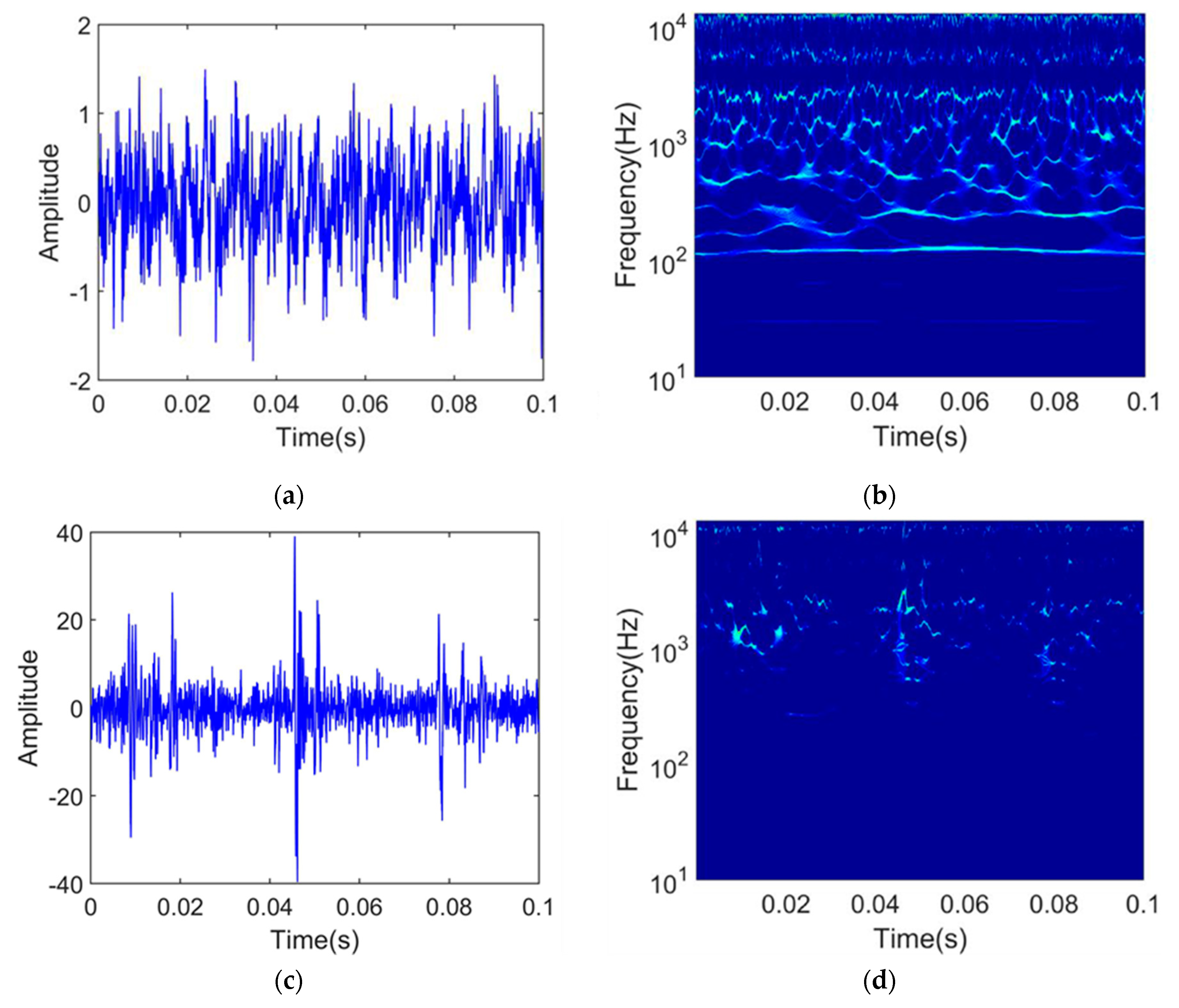
2.1. Synchrosqueezed Wavelet Transforms

Bearing degradation signal is complex and nonstationary, time–frequency domain features can represent such kind of information effectively. Wavelet transform (WT) is a common time–frequency analysis technique, which is widely applied in the condition monitoring of rotating machinery. However, the traditional WT has the disadvantages of low time–frequency resolution, and the signal features are fuzzy in time–frequency domain, which has a negative impact on the degraded feature extraction of bearings.

Synchrosqueezed Wavelet Transforms (SWT) [20] is a time–frequency rearrangement method based on traditional wavelet transform (WT), using the characteristic that the phase of the signal is not affected by the scale transformation in the frequency domain after WT to obtain the corresponding frequency at each scale. Then, the scale of the same frequency is added, and the wavelet coefficients obtained by WT are redistributed and compressed so that the value near the frequency is compressed into the frequency. SWT mainly includes the following steps. Firstly, the continuous wavelet transform is applied to the signal

$$W_x\left(a,b\right)=a^{-\frac{1}{2}}{\displaystyle {\int }_{-\infty }^{+\infty }x\left(t\right)}\overline{\psi }\left(\frac{t-b}{a}\right)dt$$

(1)

where a is the scaling parameter, b is the translating parameter, $x\left(t\right)$ is a 1-D degradation signal. $\psi \left(t\right)$ is the complex conjugate of mother wavelet function. Then instantaneous frequency ${\omega }_x\left(a,b\right)$ for the signal x is calculated by

$${\omega }_x\left(a,b\right)=-i{\left(W_x\left(a,b\right)\right)}^{-1}\frac{\partial }{\partial b}{W}_x\left(a,b\right).$$

(2)

The information is transferred from the time–scale plane to the time–frequency plane, according to the map $\left(b,a\right)\to \left(b,{\omega }_x\left(a,b\right)\right)$. $W_x\left(a,b\right)$ is computed only at discrete values $a_k$, with $a_k-a_{k-1}={\left(\Delta a\right)}_k$, and its synchrosqueezed transform $T_X\left({\omega }_l,b\right)$ was likewise determined only at the centers ${\omega }_l$ of the successive bins $\left[{\omega }_l-\Delta \omega /2,{\omega }_l+\Delta \omega /2\right]$, with ${\omega }_l-{\omega }_{l-1}=\Delta \omega$. This process is expressed as

$$T_x\left({\omega }_l,b\right)={\left(\Delta \omega \right)}^{-1}{\displaystyle \sum _{a_k:\left|{\omega }_x\left(a,b\right)-{\omega }_l\right|\le \Delta \omega /2}{W}_x\left(a,b\right)}{a}_k{}^{-3/2}\Delta a_k.$$

(3)

In this way, each frequency component in the signal is compressed in the frequency domain direction, and the problem of the low resolution of the traditional WT in the time–frequency domain is solved.

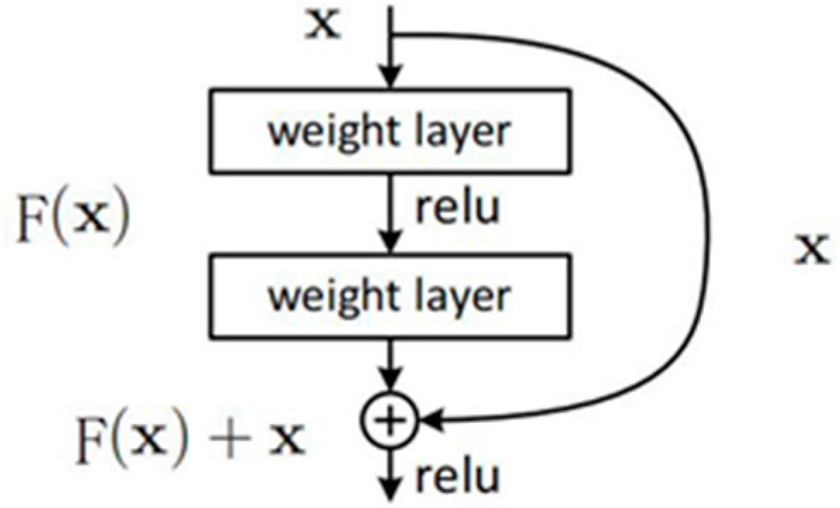
2.2. Deep Residual Convolutional Neural Networks

Because the bearing degradation process has strong nonlinear characteristics, the shallow, deep learning model is difficult to find the optimal results. Increasing the width and depth of traditional CNN can improve network performance, but with the increase in network layers, some local features are lost, and there are problems such as gradients disappearance and explosion [21]. The residual network structure [22] effectively solves these problems and significantly improves model performance. The residual network consists of a series of residual blocks, as shown in Figure 1, which can be expressed as

$$y=F\left(x,\left\{W_i\right\}\right)+x$$

(4)

where x and y are the input and output vectors of the corresponding network layer, respectively, the function $F\left(x,\left\{W_i\right\}\right)$ represents the residual mapping to be learned. The shortcut connections introduce neither extra parameter nor computation complexity, and the performance degradation of traditional neural networks with increasing depth is solved.

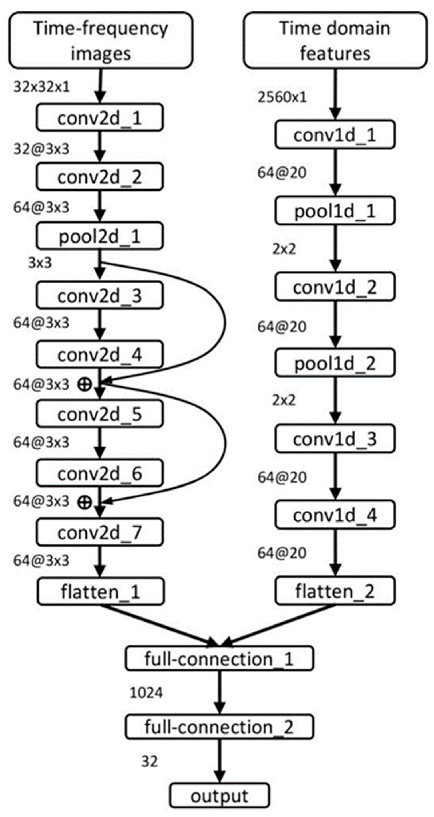
2.3. Parallel Network Structure

The time-domain features contain the time-dependent vibration characteristics, and the time–frequency domain features can effectively reveal the nonstationary characteristics of the bearing degradation signals. The collected bearing vibration signals are one-dimensional time series, while the time–frequency images are two-dimensional, and the forms of the features are quite different. The traditional processing method is to manually extract partial degradation features and combine them into a one-dimensional sequence for analysis [16,23] or only use one domain feature for analysis [12,13], which cannot guarantee the comprehensiveness of degradation information.

In this paper, the time-domain features and the time–frequency images are combined as input by using the P-ResNet. One-dimensional convolution operation of the time domain features and two-dimensional convolution operation of the time–frequency images are carried out to ensure the comprehensiveness of the bearing degradation information. The structure of the P-ResNet model is shown in Figure 2. The corresponding networks of time–frequency images include seven two-dimensional convolutional layers, a two-dimensional pooling layer, two residual layers, and a flattened layer. The corresponding networks of the time domain features include four one-dimensional convolutional layers, two one-dimensional pooling layers, and a flattened layer. Then the two flattened layers are combined into a one-dimensional vector as the input of the fully connected layer. Finally, the RUL is predicted through three fully connected layers.

3. Proposed Method

3.1. Flow Chart

Figure 3 presents the flow chart of the proposed prognostic method. The collection of bearing vibration signals is performed by sensors. In most instances, the state of the bearing is stable at the initial stage of operation, and the bearing can be considered healthy without the need for accurate RUL estimation. If a certain threshold value indicating the start of degradation is reached, an accurate prediction is performed, and the time corresponding to the threshold value is expressed as the start prediction time (SPT).

After collecting the original vibration data of the bearing, SPT is first determined. The data after SPT are transformed by SWT to obtain the time–frequency images. The time-domain characteristics and time–frequency images are input into the regression model for training and RUL prediction.

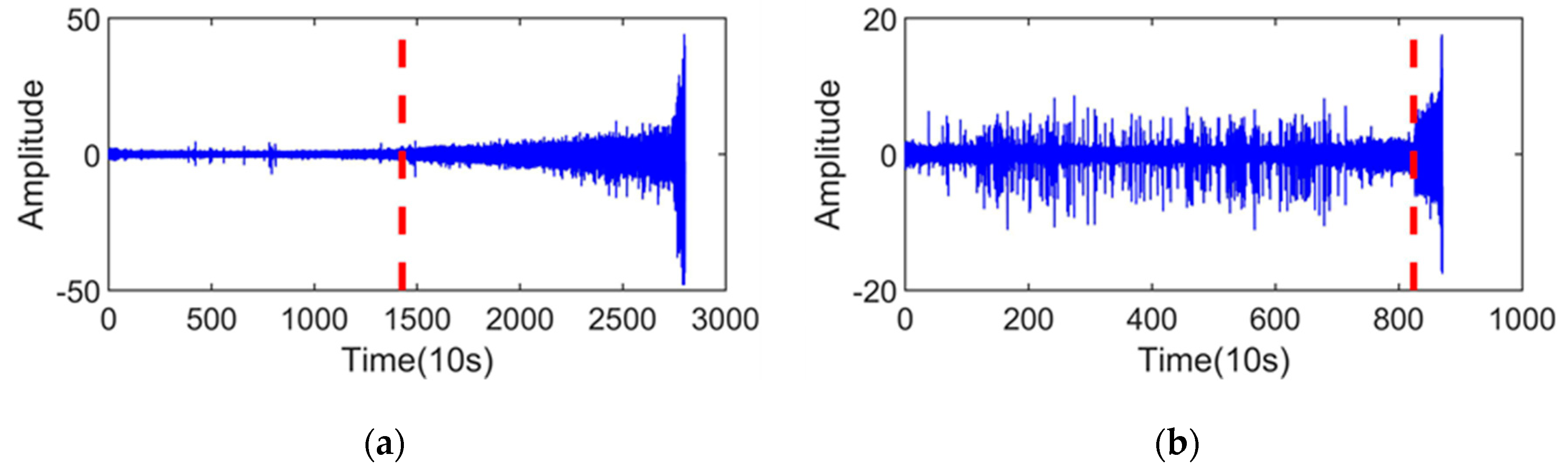
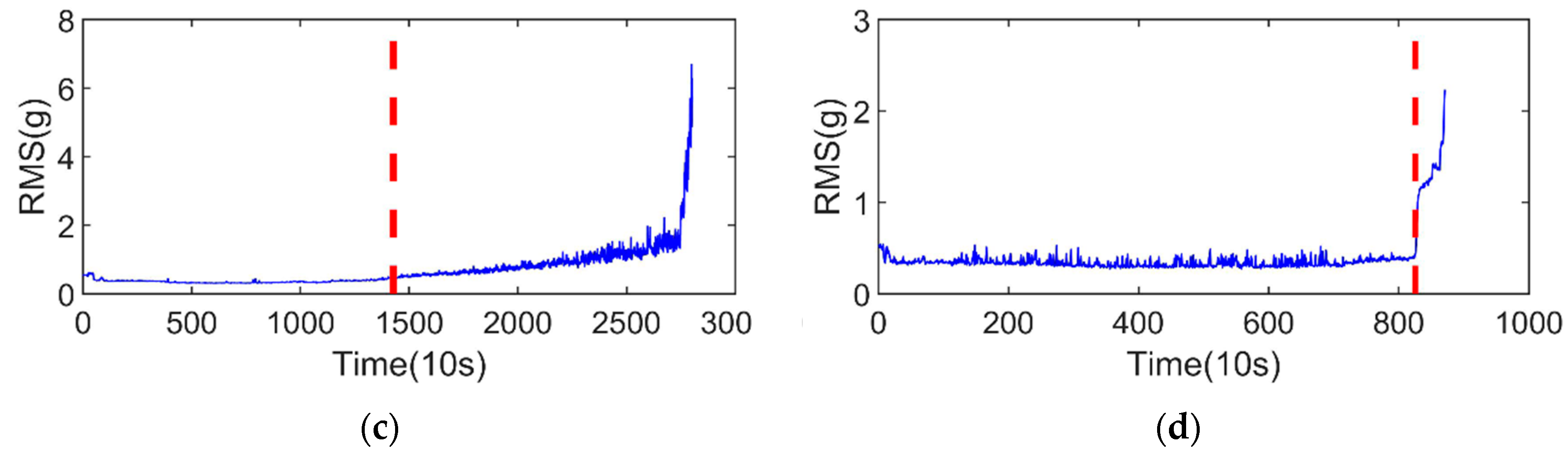
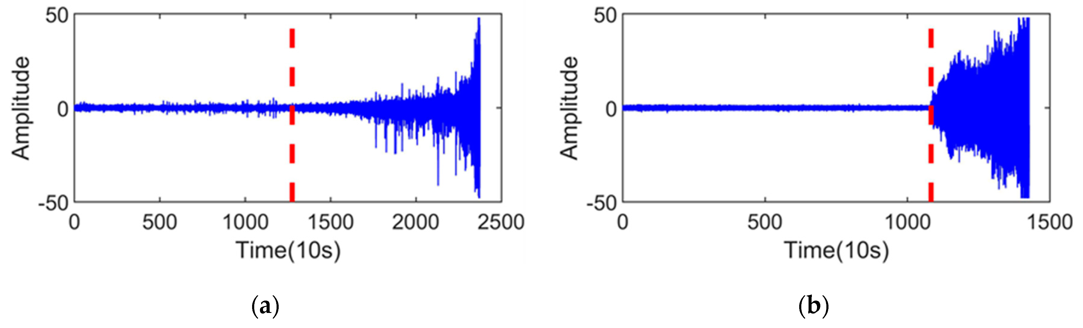
3.2. SPT Determination

The bearing vibration signal before SPT rarely contains information about bearing degradation; it is very important to determine SPT, which affects the accuracy of RUL estimation [24]. The root mean square (RMS) is the most appropriate indicator of bearing health because it shows the trends of the different health statuses of the bearing: in the normal stage, the RMS remains stable; in the initial degradation stage, the RMS starts linear growth; in the severe degradation stage, the RMS starts nonlinear growth, but there are some outliers caused by random noises in the RMS.

This paper adopts a simple and effective method to determine the SPT. At the initial stage of bearing operation, the RMS of the bearing vibration signal and its mean value $\mu$ and variance $\sigma$ were calculated. Then the moving average (MA) method is used to compute the RMS mean value ${\mu }_i$ of the next five consecutive samples; when $\left|{\mu }_i-\mu \right|>3\sigma$, the time corresponding to the maximum sample of the five samples is selected as SPT. Experiments show that the method effectively filters out RMS abnormal points.

3.3. Training Details of Neural Network Model

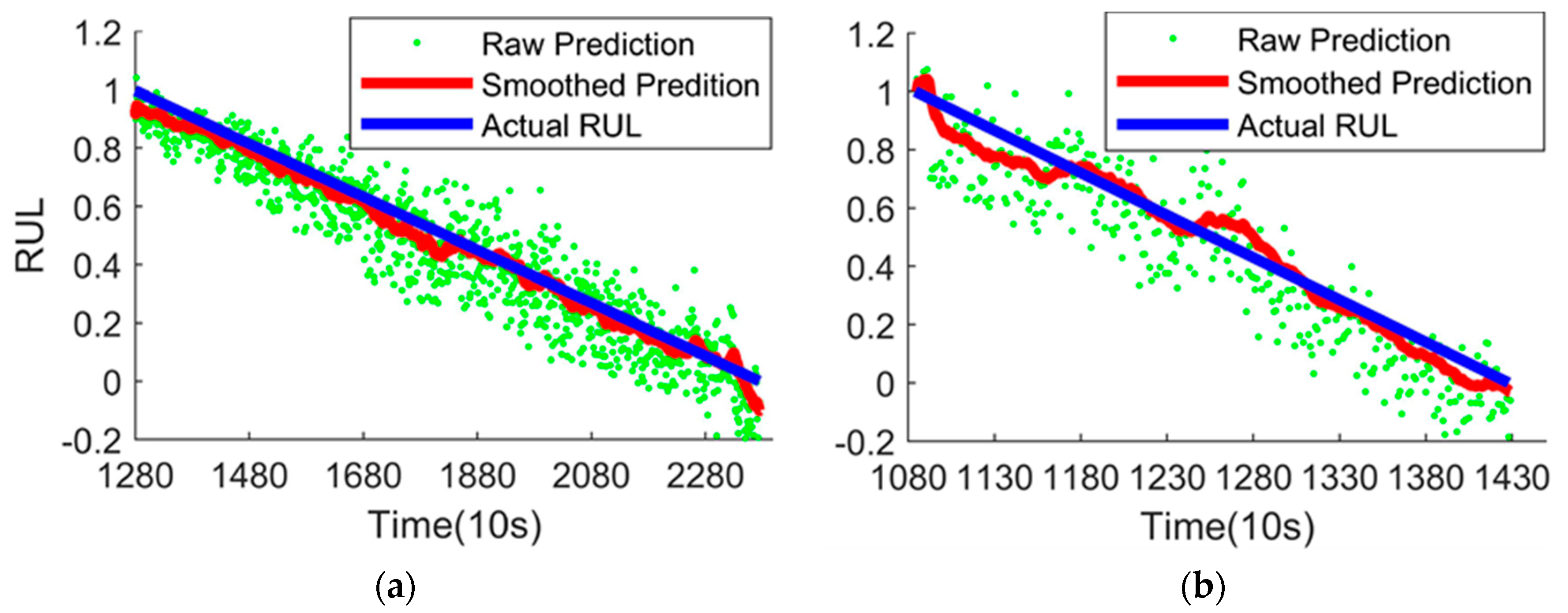
The structure of P-ResNet is shown in Figure 2. The input layer consists of two parts, the size of the time–frequency images is 32 × 32, and the size of the time-domain feature is 2560 × 1. In order to avoid the problems of gradient vanishing or explosion, the whole model uses rectified linear units (ReLU) as the activation function. In order to solve the instability of RUL prediction and obtain more accurate results, the RUL percentage is used as the label of bearing data. First, determine the SPT of training data, then the labels corresponding to the training data are set to be linearly decreasing,

$$y_i=R_i=1-\frac{T_i-T_1}{T_e-T_1}$$

(5)

where $y_i$ is the label of the input at time $t_i$, $R_i$ is the RUL percentage of the training data at time $t_i$. $T_e$ is the total time of the test; $T_1$ is the SPT, $T_i$ is the run time for now. The model first evaluates the level of degradation of bearing performance and then maps the RUL percentage to bearing RUL.

Because RUL prediction is a regression problem, mean square error (MSE) [25], which has the advantage of a fast convergence rate, is quite a suitable loss function to adopt for the model,

$$L\left(\widehat{y},y\right)=\frac{1}{m}{{\displaystyle \sum _{i=1}^m\left({\widehat{y}}_i-y_i\right)}}^2$$

(6)

where m is the batch size and ${\widehat{y}}_i$ represents the corresponding RUL percentage prediction by the P-ResNet, $y_i$ denotes the actual RUL percentage of the ith sample.

In the model training, the model parameters are updated by the back propagation algorithm, and the loss function is iteratively minimized by the Adam optimization algorithm [26]. The weights of all layers are initialized with a mean value of 0 and a standard deviation of 0.01. The biases are initialized with 0. The learning rate is set to 0.01, each batch contains 32 samples, and the number of training epochs is 1000.

3.4. Smoothing

The RUL prediction by the regression model usually has local fluctuations, but the actual bearing RUL has a linear relationship with the running time. In order to reduce the measurement noise and other uncertainties to obtain more accurate results, the KF algorithm [27] is adopted. The KF algorithm consists of two stages: prediction and measurement update. The equations for the prediction stage are

$$\begin{array}{l}{x}_{t|t-1}=x_{t-1|t-1}\\ P_{t|t-1}=P_{t-1|t-1}+Q\\ K_t=P_{t|t-1}{\left(P_{t|t-1}+R_t\right)}^{-1}\\ x_{t|t}=x_{t|t-1}+K_t\left({\widehat{y}}_t-x_{t|t-1}\right)\end{array}$$

(7)

where $x_{t|t-1}$ is the RUL prediction using the previous RUL, $x_{t-1|t-1}$ is the best RUL prediction at time $t-1$, $P_{t|t-1}$ is the variance of $x_{t|t-1}$, Q is the variance of system process, $K_t$ is Kalman gain, $R_t$ is the variance of measurement noise. ${\widehat{y}}_t$ represents the bearing RUL at time t obtained by the P-ResNet model. $x_{t|t}$ is the optimized predicted value obtained by KF at time t. The variance update process is

$$P_{t|t}=\left(1-K_t\right)P_{t|t-1}$$

(8)

where $P_{t|t}$ is the variance of $x_{t|t}$. The initial value $x_0$ is set to be 1, Q is set to be 1 × 10⁻⁴, and $R_0$ is set to be 4 × 10⁻³.

4. Experimental Study

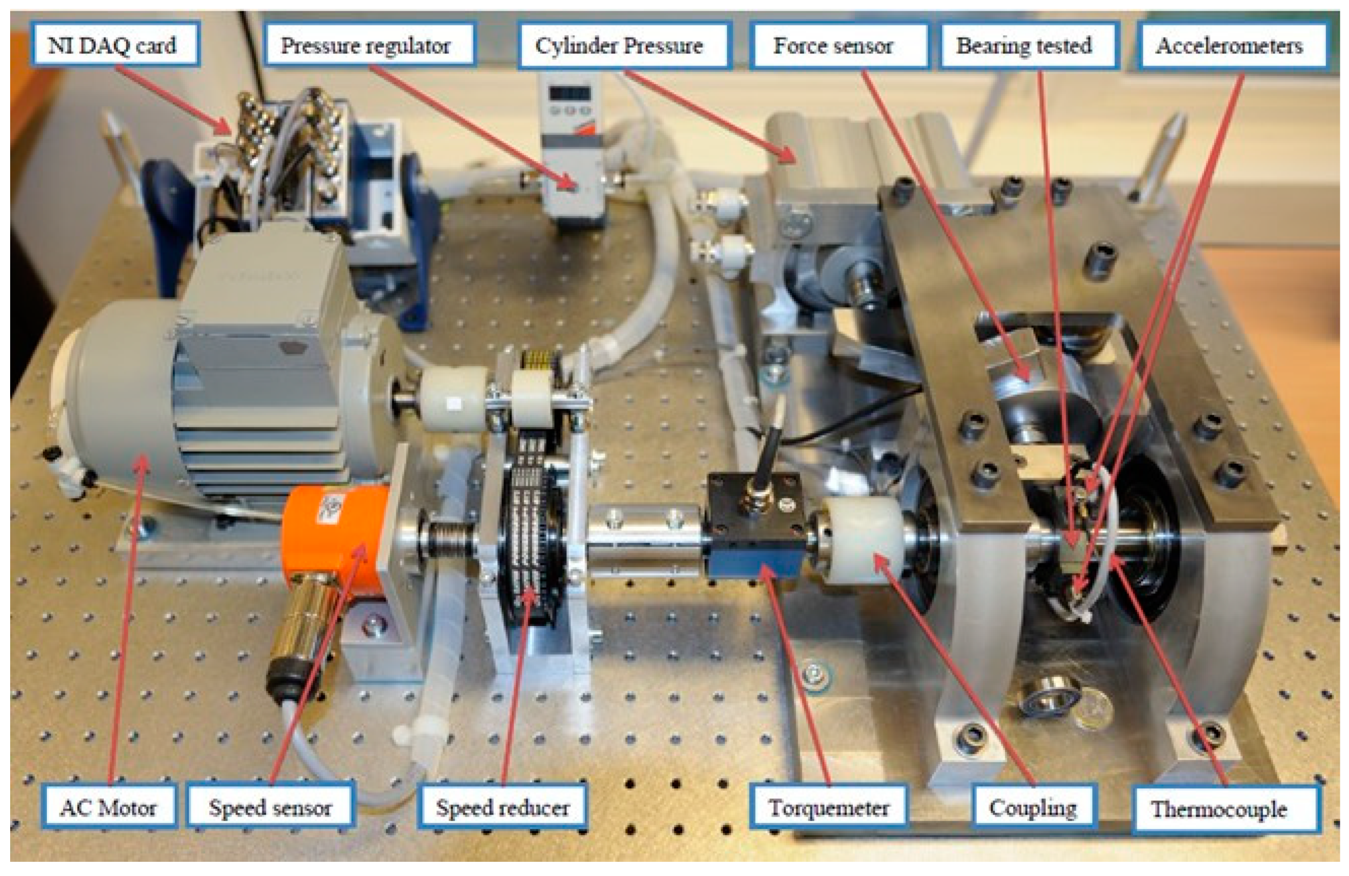
4.1. Dataset Description

The experimental data were collected from PRONOSTIA in the IEEE PHM 2012 Data Challenge [28]. During the experiments, a radial force of 4 kN was applied to the test bearings for accelerated life testing. The rotating speed of bearings is 1800 r/min. In order to monitor the degradation process, the bearing was installed with two acceleration sensors, where one was set on the vertical axis, and the other one was on the horizontal axis. The sampling frequency of the vibration signal is 25.6 kHz, 2560 data points were recorded at 0.1 s per sampling, and the recording interval is 10 s. When the amplitude of the vibration signal exceeded 20 g, the bearing was considered invalid, and the experiment was stopped. The PRONOSTIA platform is shown in Figure 4.

In this paper, the signals collected in the horizontal direction were used for analysis. The bearing1_1 and bearing1_2, which contain a total of 3674 samples, were used as training sets, and the bearing1_3 in size of 1802 samples and bearing1_4 in size of 1139 samples were used as test sets.

Matlab was used for data preprocessing, including SPT determination, SWT and PCA dimension reduction, as well as for plotting the diagrams. Tensorflow framework was used for implementing the P-ResNet, model training and testing.

4.2. Experimental Process

The vibration signals of the training sets are shown in Figure 5a,b, and the RMS of the training sets are shown in Figure 5c,d. First was determining the SPT of the training sets, which is indicated by the red dashed line in Figure 4. It was observed that the SPT of the two bearings is 1427 and 824, respectively.

After the SPT was determined, the data after SPT were processed. Each sample has 2560 points, which can be directly used as the time domain features to input the regression model. The training sets are transformed into time–frequency images by SWT. In order to illustrate the frequency energy change with regard to time, the vibration signals and time–frequency images of the first and last samples of bearing1_1 are shown in Figure 6. From Figure 6, we can see that the frequency fluctuations in the time–frequency image of the bearing in the initial degradation stage are not obvious. However, in the final stage, defective bearings appear periodic pulse phenomenon. These time–frequency images 320 × 2560 are resized to 32 × 32 to form a standard image size using principal component analysis (PCA), which is used as input of the regression model. The time-domain features and time–frequency images, and corresponding labels are used to train the regression model. After model training is finished, the RUL of test sets can be predicted.

The vibration signals of the test sets are shown in Figure 7a,b, and the RMS of the test sets are shown in Figure 7c,d. First, the SPT of the test sets was determined, which is indicated by the red dashed line in Figure 7. The test samples after SPT were processed in the same way as the training sets, and then input into the regression model for RUL prediction.

The RUL prediction results of the test sets are shown in Figure 8. It can be seen from Figure 8 that the smoothed prediction curve is quite close to the actual RUL, which can prove that the proposed method is effective for detecting the bearing degradation trend and predicting RUL.

4.3. Comparisons with Different Methods

A comparison of the RUL prediction results with results from the other three methods is presented so as to evaluate the performance of the proposed method comprehensively. The first method [14] relies on time–frequency images and CNN to predict bearing RUL. The second method [10] uses the time domain characteristics of bearing vibration signals and CNN to predict the bearing RUL. The third method [7] uses SVR to predict bearing RUL.

The commonly used performance comparison indexes are mean absolute error (MAE) and root mean square error (RMSE), which are defined as

$$\mathrm{MAE}=\frac{1}{m}{\displaystyle \sum _{i=1}^m\left|{\widehat{y}}_i-y_i\right|},$$

(9)

$$\mathrm{RMSE}=\sqrt{\frac{1}{m}{{\displaystyle \sum _{i=1}^m\left({\widehat{y}}_i-y_i\right)}}^2}$$

(10)

where m is the number of samples in the test sets and ${\widehat{y}}_i$ represents the corresponding RUL percentage estimation by the deep neural network, $y_i$ denotes the actual RUL percentage of the ith sample, the comparison results are shown in

Table 1. Numerical prognostic performance comparisons of different methods.

		The Proposed Method	Time–Frequency Features + CNN	Time Domain Features + CNN	SVR
Bearing1_3	MAE	0.09	0.12	0.15	0.14
	RMSE	0.12	0.16	0.22	0.31
Bearing1_4	MAE	0.17	0.73	0.31	0.25
	RMSE	0.23	0.26	0.28	0.36

. It can be clearly seen that the MAE and RMSE value performed by the proposed method is smaller than those performed by the other three methods. By taking the MAE value as the standard, the RUL prediction accuracy of the proposed method was improved by at least 3% compared with the other three methods. With the RMSE value as the standard, there is also at least a 3% accuracy improvement of the proposed method compared with the other three methods.

The comparison with the time–frequency features + CNN method shows that the proposed method have more robustness for different test set [18] and a small increase in prediction accuracy, which proves that learning two domain types of features in parallel is more comprehensive and more robust for RUL prediction. Compared with the time-domain features + CNN method, the prediction accuracy of the proposed method has a quite sufficient increase, which proves that the time–frequency features are important to consider. The last comparison with the SVR method shows the defects of traditional machine learning to learn complex features.

5. Conclusions

In this paper, a bearing RUL prediction method based on P-ResNet was proposed. During machine operation, the start prediction time was firstly determined by an RMS-based moving average method. Then, the time–frequency domain images of raw data were obtained by synchrosqueezed wavelet transform (SWT). To ensure the comprehensiveness of the bearing degradation information and improve the accuracy of the RUL prediction, the time domain features of bearing vibration signals and the time–frequency images were both used as the inputs of the parallel convolutional network model, which can learn those two types of features with two different series of convolutional operations in parallel. The residual network layers in the regression model enhance the learning ability. Finally, the KF algorithm is used to maintain the stability of the predicted results. In order to verify the performance of the proposed method, the IEEE PHM 2012 Data Challenge dataset was adopted for experimental study. The experimental results prove that the proposed method is effective for bearing RUL prediction. Compared with the other three methods, at least a 3% accuracy improvement proved that the proposed method has certain superiority.

The advantages of the proposed methods are summarized as follows. (1) Synchrosqueezed wavelet transform (SWT), which overcomes the low time–frequency resolution of the traditional wavelet transform, was adopted to obtain time–frequency domain features of vibration signals. With both time–frequency domain features and time-domain features as training data, the comprehensiveness of bearing degradation information can be ensured. (2) A parallel deep residual convolutional neural network (P-ResNet) was used for training and RUL prediction. In the structure of P-ResNet, there are two parallel series of convolutional layers to learn time–frequency domain features and time-domain features, respectively, and residual layers to enhance the learning ability, which can obtain a more accurate trained model for RUL prediction. (3) The KF algorithm was adopted for smoothing the predicted results, which can effectively reduce the measurement noises and other uncertainties.

In terms of practical application, the proposed method can be applied to the rolling bearing RUL prediction for equipment in the fields of automobile, metallurgy, petrochemical, and so on to reduce the probability of bearing failure, improve the reliability of equipment and finally reduce economic losses for enterprises.

There are two directions for our further research on this work. First of all, to verify different components of the RUL prediction performance of the proposed method, more vibration signal datasets collected from different equipment components such as gear and worm must be used for training the proposed model, which adjusted the parameters. Secondly, in order to be applied to the RUL prediction of bearing under different working conditions, the proposed model will be improved with unsupervised domain adaptation.

References

1. Zhao, Z.; Quan, Q.; Cai, K.Y. A profust reliability based approach to prognostics and health management. IEEE Trans. Rel. 2014, 63, 26–41. [Google Scholar] [CrossRef]
2. Heng, A.; Zhang, S.; Tan, A.C.C.; Mathew, J. Rotating machinery prognostics: State of the art, challenges and opportunities. Mech. Syst. Signal Process. 2009, 23, 724–739. [Google Scholar] [CrossRef]
3. Tian, Z.G.; Liao, H.T. Condition based maintenance optimization for multi-component systems using proportional hazards model. Reliab. Eng. Syst. Saf. 2011, 96, 581–589. [Google Scholar] [CrossRef]
4. Gebraeel, N.; Lawley, M.; Liu, R.; Parmeshwaran, V. Residual life predictions from vibration-based degradation signals: A neural network approach. IEEE Trans. Ind. Electron. 2004, 51, 694–700. [Google Scholar] [CrossRef]
5. Ali, J.B.; Chebel-Morello, B.; Saidi, L.; Malinowski, S.; Fnaiech, F. Accurate bearing remaining useful life prediction based on Weibull distribution and artificial neural network. Mech. Syst. Signal Process. 2015, 56, 150–172. [Google Scholar]
6. Chen, X.; Xiao, H.; Guo, Y.; Kang, Q. A multivariate grey RBF hybrid model for residual useful life prediction of industrial equipment based on state data. Int. J. Wirel. Mob. Comput. 2016, 10, 90–96. [Google Scholar] [CrossRef]
7. Loutas, T.H.; Roulias, D.; Georgoulas, G. Remaining useful life estimation in rolling bearings utilizing data-driven probabilistic E-support vectors regression. IEEE Trans. Rel. 2013, 62, 821–832. [Google Scholar] [CrossRef]
8. Song, Y.; Liu, D.; Hou, Y.; Yu, J.; Peng, Y. Satellite lithium-ion battery remaining useful life estimation with an iterative updated RVM fused with the KF algorithm. Chin. J. Aeronaut. 2018, 31, 31–40. [Google Scholar] [CrossRef]
9. Liu, R.; Yang, B.; Zio, E.; Chen, X. Artificial intelligence for fault diagnosis of rotating machinery: A review. Mech. Syst. Signal Process. 2018, 108, 33–47. [Google Scholar] [CrossRef]
10. Babu, G.S.; Zhao, P.; Li, X.L. Deep convolutional neural network based regression approach for estimation of remaining useful life. In Proceedings of the 21st International Conference on Database Systems for Advanced Applications, Dallas, TX, USA, 16–19 April 2016. [Google Scholar]
11. Zhu, J.; Chen, N.; Peng, W. Estimation of bearing remaining useful life based on multiscale convolutional neural network. IEEE Trans. Ind. Electron. 2019, 66, 3208–3216. [Google Scholar] [CrossRef]
12. Li, X.; Zhang, W.; Ding, Q. Deep learning-based remaining useful life estimation of bearings using multi-scale feature extraction. Reliab. Eng. Syst. Saf. 2019, 182, 208–218. [Google Scholar] [CrossRef]
13. Yang, B.; Liu, R.; Zio, E. Remaining useful life prediction based on a double-convolutional neural network architecture. IEEE Trans. Ind. Electron. 2019, 66, 9521–9530. [Google Scholar] [CrossRef]
14. Luo, J.; Zhang, X. Convolutional neural network based on attention mechanism and Bi-LSTM for bearing remaining life prediction. Appl. Intell. 2022, 52, 1076–1091. [Google Scholar] [CrossRef]
15. Ren, L.; Cui, J.; Sun, Y.; Cheng, X. Multi-bearing remaining useful life collaborative prediction: A deep learning approach. J. Manuf. Syst. 2017, 43, 248–256. [Google Scholar] [CrossRef]
16. Cheng, Y.; Hu, K.; Wu, J.; Zhu, H.; Lee, C.K.M. A deep learning-based two-stage prognostic approach for remaining useful life of rolling bearing. Appl. Intell. 2022, 52, 5880–5895. [Google Scholar] [CrossRef]
17. Huang, R.; Xi, L.; Li, X.; Liu, R.; Qiu, H.; Lee, J. Residual life predictions for ball bearings based on self-organizing map and back propagation neural network methods. Mech. Syst. Singal Process. 2007, 21, 193–207. [Google Scholar] [CrossRef]
18. Wang, X.; Wang, T.; Ming, A.; Han, Q.; Chu, F.; Zhang, W.; Li, A. Deep spatiotemporal convolutional-neural-network-based remaining useful life estimation of bearings. Chin. J. Mech. Eng. 2021, 34, 62–76. [Google Scholar] [CrossRef]
19. Cao, Y.; Ding, Y.; Jia, M.; Tian, R. A novel temporal convolutional network with residual self-attention mechanism for remaining useful life prediction of rolling bearings. Reliab. Eng. Syst. Safe. 2021, 215, 107813. [Google Scholar] [CrossRef]
20. Daubechies, I.; Lu, J.; Wu, H.T. Synchrosqueezed wavelet transforms: An empirical mode decomposition-like tool. Appl. Comput. Harmon. Anal. 2011, 30, 243–261. [Google Scholar] [CrossRef] [Green Version]
21. Glorot, X.; Bengio, Y. Understanding the difficulty of training deep feedforward neural networks. In Proceedings of the 13th International Conference on Artificial Intelligence and Statistics, Sardinia, Italy, 13–15 May 2010. [Google Scholar]
22. He, K.; Zhang, X.; Ren, S.; Sun, J. Deep Residual Learning for Image Recognition. In Proceedings of the 2016 IEEE Conference on Computer Vision and Pattern Recognition (CVPR), Las Vegas, NV, USA, 27–30 June 2016; pp. 770–778. [Google Scholar]
23. Ren, L.; Cheng, X.; Wang, X.; Cui, J.; Zhang, L. Multi-scale dense gate recurrent unit networks for bearing remaining useful life prediction. Future Gener. Comput. Sys. 2019, 94, 601–609. [Google Scholar] [CrossRef]
24. Ahmad, W.; Khan, S.A.; Kim, J.M. A hybrid prognostics technique for rolling element bearings using adaptive predictive models. IEEE Trans. Ind. Electron. 2018, 65, 1577–1584. [Google Scholar] [CrossRef]
25. Picking Loss Functions—A Comparison Between MSE, Cross Entropy and Hinge Loss. Available online: https://rohanvarma.me/Loss-Functions/ (accessed on 14 April 2022).
26. Kingma, D.; Ba, J. Adam: A method for stochastic optimization. arXiv 2014, arXiv:1412.6980. [Google Scholar]
27. Kalman, R.E. A new approach to linear filtering and prediction problems. ASME. J. Basic Eng. 1960, 82, 35–45. [Google Scholar] [CrossRef] [Green Version]
28. Nectoux, P.; Gouriveau, R.; Medjaher, K.; Ramasso, E.; Morello, B.; Zerhouni, N.; Varnier, C. PRONOSTIA: An experimental platform for bearings accelerated degradation tests. In Proceedings of the 2012 IEEE International Conference on Prognostics and Health Management, Denver, CO, USA, 18–21 June 2012. [Google Scholar]
Figure 1. Residual block.
Applsci 12 04299 g001
Figure 2. P-ResNet structure.
Applsci 12 04299 g002
Figure 3. Flow chart of the proposed method for prognostics.
Applsci 12 04299 g003
Figure 4. The PRONOSTIA platform.
Applsci 12 04299 g004
Figure 5. Vibration signals of the training sets and their RMS: (a) vibration signal of the bearing1_1; (b) vibration signal of the bearing1_2; (c) RMS of the bearing1_1; and (d) RMS of the bearing1_2.
Applsci 12 04299 g005aApplsci 12 04299 g005b
Figure 6. Bearing 1_1: (a) Waveform for the first sample; (b) time–frequency images for the first sample; (c) waveform for the last sample; and (d) time–frequency images last sample.
Applsci 12 04299 g006
Figure 7. Vibration signals of the test sets and their RMS: (a) vibration signal of the bearing1_3; (b) vibration signal of the bearing1_4; (c) RMS of the bearing1_3; and (d) RMS of the bearing1_4.
Applsci 12 04299 g007aApplsci 12 04299 g007b
Figure 8. RUL prediction results of the test sets. (a) RUL prediction results of the Bearing1_3 by the proposed method; (b) RUL prediction results of the Bearing1_4 by the proposed method.
Applsci 12 04299 g008