Forecasting Fine-Grained Air Quality for Locations without Monitoring Stations Based on a Hybrid Predictor with Spatial-Temporal Attention Based Network

Abstract

Air pollution in cities is a severe and worrying problem because it causes threats to economic development and health. Furthermore, with the development of industry and technology, rapid population growth, and the massive expansion of cities, the total amount of pollution emissions continue to increase. Hence, observing and predicting the air quality index (AQI), which measures fatal pollutants to humans, has become more and more critical in recent years. However, there are insufficient air quality monitoring stations for AQI observation because the construction and maintenance costs are too high. In addition, finding an available and suitable place for monitoring stations in cities with high population density is difficult. This study proposes a spatial-temporal model to predict the long-term AQI in a city without monitoring stations. Our model calculates the spatial-temporal correlation between station and region using an attention mechanism and leverages the distance information between all existing monitoring stations and target regions to enhance the effectiveness of the attention structure. Furthermore, we design a hybrid predictor that can effectively combine the time-dependent and time-independent predictors using the dynamic weighted sum. Finally, the experimental results show that the proposed model outperforms all the baseline models. In addition, the ablation study confirms the effectiveness of the proposed structures.

1. Introduction

In recent years, with the increasing development of industry and technology, the rapid growth of the population, and the massive expansion of cities, air pollution has become significantly worse and threatens both health and economy. For example, PM_2.5, which consists of particles less than 2.5 μm, is fatal and leads to cardiovascular disease or respiratory illness [1]. Hence, an air quality index (AQI) is used by government agencies (https://www.airnow.gov/aqi/aqi-basics/) (accessed on 17 April 2022) to communicate to the public how polluted the air currently is or how polluted it is forecast to become. By monitoring AQI levels, the government and citizens can forecast air quality and thus take significant actions in advance to prevent being affected by air pollution. Even though the demand to forecast the air quality has increased, forecasting air quality is still challenging for several reasons. Air quality values vary significantly over time and across locations because of various complicated factors, such as meteorological effects, surrounding land usages, and the daily behaviors of people. Moreover, sudden changes and accidents might affect the air quality as well and thus make it difficult for a general air quality prediction model to accurately forecast the future. For example, an industrial accident such as a fire in a factory might cause the concentration of pollutants to increase rapidly. Conversely, the outbreak of widespread diseases like COVID-19 [2] might decrease pollution emissions because of substantially reduced human activities.

In general, air quality prediction in cities has focused on two conditions. One is to predict future air pollution in areas with monitoring stations, known as the air pollution forecasting problem. This problem has been widely discussed and has had many high-performance solutions in recent research [3,4]. The other condition is to estimate air pollution in areas without monitoring stations in the current hour, also known as fine-grained air pollution estimation [5,6]. The second condition is also more challenging because there is no sufficient labeled data to train an effective module [5]. In the real world, monitoring stations are usually insufficient and sparsely distributed in a large city because of the high construction and maintenance costs. In addition, suitable places in densely populated cities are rare and unavailable. As a result, people have to analyze and predict the current fine-grained AQI with limited historical data.

Traditionally, researchers [7,8,9] used historical air pollution data crawled from established monitoring stations to predict air quality. However, with the increasing amount of open data and sensors, people can collect more heterogeneous and dynamic data highly correlated with air pollutants. The studies [10,11] utilized these data and developed deep-learning-based models that outperform the traditional methods in air quality modeling. However, deep learning-based methods were still unable to accurately predict fine-grained air quality throughout a city because of the scarcity of air pollution monitoring stations and the incompleteness of historical data. Therefore, recently, it has become popular to discuss how existing monitoring stations can predict future air pollution levels and assess the current air pollution levels in minuscule urban areas. For example, the works [12,13] used past air quality records as a reference to calculate the spatial quality relationship between “areas with monitoring stations” and “areas without monitoring stations” and applied this relationship to predictions. Most studies have attempted to achieve the two goals stated above separately or in one model [14,15,16].

In this study, we focus on forecasting fine-grained air quality for every region, including the one without a monitoring station. The proposed model has three major components: feature extractor, inversed distance attention layer, and hybrid predictor. We use the attention layer to learn the relationship between the embedding results of the light feature extractor and the general feature extractor. Then, we apply the inversed distance as an amended coefficient to strengthen the influence of high correlation monitoring stations. Finally, the hybrid predictor generates long-term air quality predictions. To summarize, the main contributions of this study are as follows:

• To the best of our knowledge, we are the first to combine the air quality forecasting of monitoring stations, and predict the air quality of sites without monitoring stations, forecast the long-term fine-grained air quality without monitoring stations and realize the goal of long-term prediction for locations without monitoring stations.
• This study proposes a hybrid predictor with two complementary data flows that can perform well in long-term prediction for the locations without monitoring stations.
• The experimental results show that the proposed model outperforms the baseline methods. In addition, the ablation study confirms the effectiveness of the proposed structure.

The rest of this paper is organized as follows. In Section 2, we introduce the related work. We formulate the problem and introduce the data in Section 3. In Section 4, we introduce our proposed model in detail. In Section 5, we experimentally evaluate the effectiveness of the proposed solution by comparing different methods. Finally, we conclude our work with a discussion about future work in Section 6.

2. Related Work

Air pollution prediction has become a popular research topic in recent years. Researchers have proposed several methods to fulfill the objectives. In this section, we introduce the previous works of air quality forecasting, fine-grained air quality estimation, and the combination of air quality forecasting and fine-grained air quality estimation.

• Air Quality Forecasting: Previous studies have proposed many data-driven approaches for air quality modeling. For example, the work [7] introduced autoregressive integrated moving average (ARIMA), which is a famous and widely adopted data-driven model for air pollution forecast at monitoring stations. In [8], the authors proposed a traditional physical-based numerical model that used historical air pollution data [9] to formulate the urban pollution process and pollutant dispersion. Moreover, studies [3,4,17] used the combination of spatial and temporal features to model air quality forecasting. Recently, big data and neural network techniques have improved the traditional methods and achieved state-of-the-art performance in urban air quality forecasting [10,11]. Graph convolution neural network (GCN) has become particularly popular in many works. The GCN-based air quality prediction takes monitoring stations as nodes of the graph and uses static features to calculate the node embedding to forecast the predicted values [13].
• Fine-Grained Estimation: Several studies have proposed to use basic interpolation methods such as spatial averaging, nearest neighbor, inversed distance weighting (IDW), and kriging to solve the fine-grained estimation of air quality for locations without monitoring stations [18,19]. In addition, the work [5] proposed an affinity graph framework to infer real-time air quality of a location without a monitoring station, and recommend the best locations for new monitoring stations. As air quality forecasting, several studies have investigated interpolation methods using the combination of spatial and temporal features [3,6,20]. In addition, a neural network with an attention mechanism [12] has become popular for estimating the air quality of a region without monitoring stations.
• Joint Air Quality Forecasting and Fine-Grained Estimation: Few studies have attempted to achieve both air quality forecasting and fine-grained estimation. The work [15] used the combination of GCN and LSTM networks to learn the spatial–temporal correlation and then predict these two targets. The work in [16] proposed a hybrid model to perform feature selection, air quality forecasting, and fine-grained estimation jointly in one single model. Moreover, the studies in [14,21] show that using air quality forecasting and fine-grained estimating as multi-task learning can improve the generalization performance by leveraging the commonalities and differences between these two tasks.

Although previous studies [14,16] have proposed methods to jointly model air quality forecasting and fine-grained estimation and enhance the performance, there is still much for improvement. For example, these methods do not solve long-term prediction challenges in regions without sufficient historical data or monitoring stations. To solve this problem, we propose a model that can capture the complex spatial and temporal interaction between air pollution and geographical data, and then predict the air quality in places without sufficient historical data.

3. Preliminaries

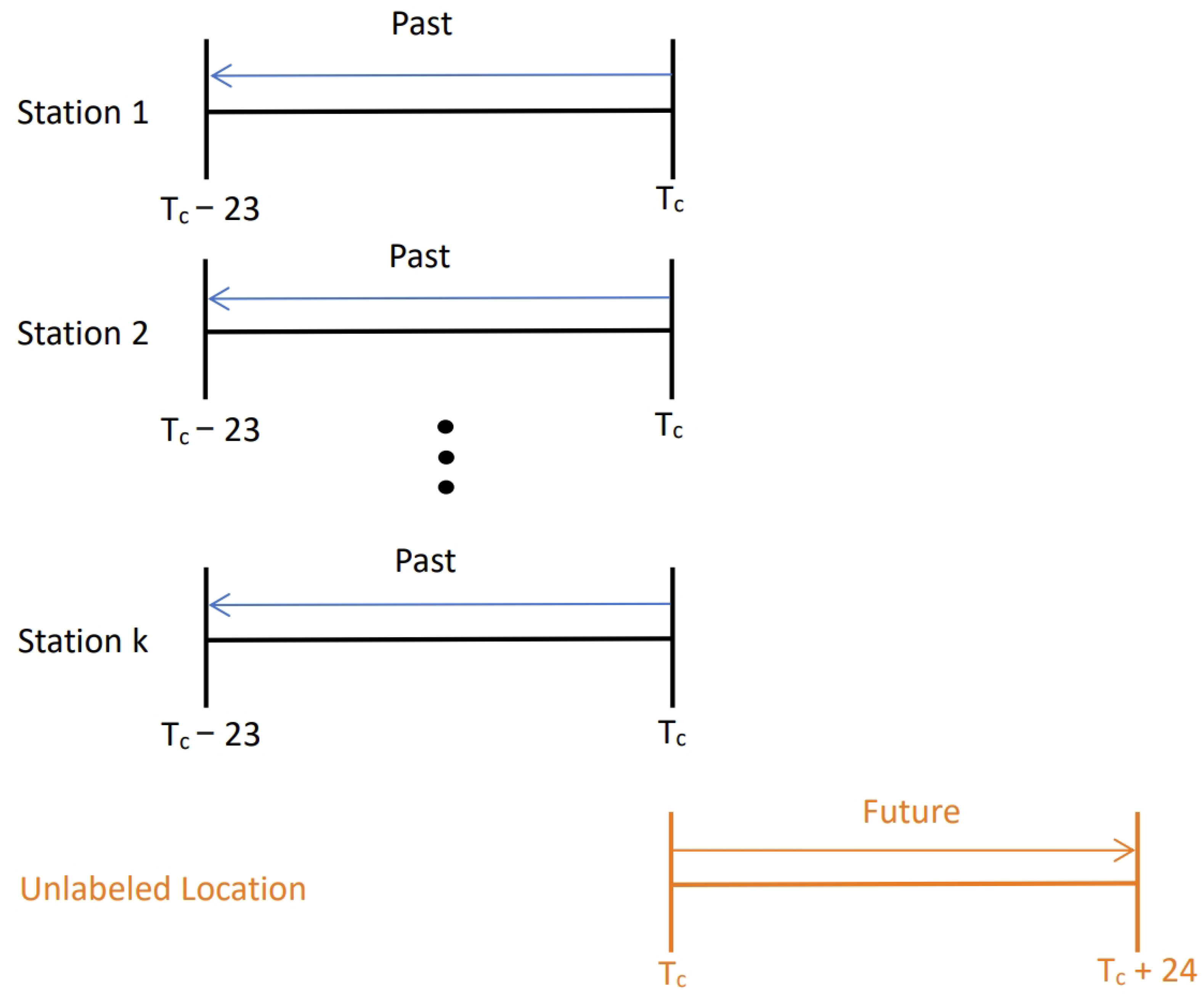
3.1. Problem Statement

We divide cities into disjoint grids (e.g., 2.2 km × 2.2 km). Let U and S represent the lack and the existence of air quality monitoring stations separately. Given a grid $G_U$ and a set of grids $G_S={\left\{G_{Sn}\right\}}_{(n=1)}^K$, where K is the number of monitoring stations, our goal is to infer future AQI of $G_U$ (say, next 24 h) based on historical and current dynamic and static features of $G_U$ and $G_S$.

3.2. Definition of Input Features

In this study, we aim to infer spatially fine-grained city air quality value based on existing air quality monitoring stations and achieve a long-term prediction on areas without monitoring stations. The input features of the proposed model are categorized into dynamic features (i.e., AQI and meteorological data) and static features (i.e., point of interest (POIs), road network, and land use). The details of input features are as follows:

• Grid: We use longitude and latitude to divide the target area into disjoint square grids as the basic unit. Notably, we adjust the size of the grid to ensure that each grid contains only one air quality monitoring station. A grid region with no monitoring station is denoted as unlabeled grids $G_{Un}$, and a grid region with a monitoring station is denoted as labeled grids $G_{Sn}$.
• AQI: In this study, we use the dataset collected by [22]. We choose PM_2.5 values observed by air-quality monitoring stations every hour as the predictive features because PM_2.5 is the main pollutant that influences the air quality level and also the most widely used indicators of an air quality report.
• Meteorological Data: The meteorological data are critical factors to air quality level. The grid-level meteorological data in [22] includes temperature, pressure, humidity, wind direction, and wind speed.
• POIs: The amounts of POIs represent activities and the density of people in a region, which might have a huge influence on the air quality. In this study, we collect POIs data from Gaode Map and select 14 types of POIs.
• Road Network: It is known that air quality is strongly affected by traffic condition. The type and accumulated length of a road might be strongly correlated to the real-time traffic condition. In this study, the road network data are collected using OpenStreetMap and four features are identified for each grid: (1) total length of highway, (2) total length of primary road, (3) total length of secondary road, and (4) total length of the pedestrian walk.
• Land Use: The air quality of a region is highly affected by its surrounding land. For example, “Industrial Area” could be the source of air pollution; “Residential” is the place that attracts people and traffic, which worsens the air quality. Conversely, the region with a larger area of open “Green” or “Water” land might improve the air quality. In this study, we use OpenStreetMap to collect four types of land use data including (1) total area of green land, (2) total area of industrial area, (3) total area of residential area and (4) total area of waters for each grid.

4. Methodology

In this section, we introduce our proposed model to forecast the PM_2.5 values in 24 h at a target location without a monitoring station. The data preprocessing and representations of input features were described in Section 4.1. Figure 1 presents the overview of our proposed framework. We divide our model into three hierarchical layers including (a) feature extractor, (b) inversed distance attention, and (c) hybrid predictor. The feature extractor has two independent structures that calculate the embedding vectors of unlabeled target grids without monitoring stations and labeled grids with monitoring stations. The inversed distance attention calculates the influences of different labeled grids on unlabeled target grids. Finally, the hybrid predictor makes a long-term prediction of air quality by using the parallel structure of two independent predictors.

4.1. Data Preprocessing and Symbols

The AQI values $X^A$ collected from monitoring sensors sometimes have missing values that might decrease the performance of the model predictions. To solve this problem, a previous study [13] proposed replacing the missing values by computing the mean value in a six-hour sliding window. For example, after imputation, the missing value “NaN” in a time series of AQIs [ …, 34, 37, 46, “NaN”, 40, 31, 33, …] will be replaced by 37. Note that samples with at least two consecutive missing values are excluded from the training and testing because the artificial data might affect the effectiveness of prediction. Finally, we apply standard normalization to the AQI data.

The time series of meteorological features $X^M$ in this study have five categories: (1) temperature, (2) pressure, (3) humidity, (4) wind direction, and (5) wind speed. Among these features, only the wind direction is a categorical feature with categories, while the others are numerical. We apply one-hot encoding to the wind direction data and standard normalization to the values of numerical data.

For POI features POIs $X^P$, 14 POI categories include Company, Culture, Daily Life, Entertainment, Institution, Transportation Spots, Medical, Vehicle Service, Shopping Mall, Sports, Food and Beverage, Hotels, Education, and Financial. The POI features are the total numbers of each POI categories within the grid. After computing the POI features of all grids, the POI features are then normalized by the sum of each category among all grids so that all values are in the range of [0, 1]. For Road Networks $X^R$ and Land Use s $X^L$ features, the values are normalized to the range of [0, 1] by the total length and area of each type, respectively.

In addition, we calculate the distance between the unlabeled grid and all labeled grids by using their central latitudes and longitudes. For instance, IDW and K-NN are the common baselines for inferring fine-grained AQI from monitoring stations, and the most important key point for prediction is the distance between target regions and each monitoring station. In Equation (1), we normalize the distance between $G_U$ and $G_S$ as the Distance feature $X^D$ and yield the Inversed Distance feature $X^{ID}$ simultaneously. Normalization on the Inversed Distance feature is not performed, since the minimum Distance feature is 1.

$$\begin{array}{c}{X}^D=Normalize\left(Distance(G_U,S)\right),forSin{G}_S\\ X^{ID}=1/Distance(G_U,S),forSin{G}_S\end{array}$$

(1)

After data preprocessing, we have static features and sequential features in each grid. However, there are a few differences between input features between each grid due to the existence of monitoring stations. We extract the feature set $F_{Sn}$, which includes Meteorological $X_U^M$, POIs $X_U^P$, Road Net $X_U^R$, Land Use $X_U^L$, Distance $X_U^D$, and Inversed Distance $X_U^{ID}$ for unlabeled girds $G_U$. For a set of grids with a monitoring station, we denote them as labeled grids and use AQI $X_{Sn}^A$, Meteorological $X_{Sn}^M$, POIs $X_{Sn}^P$, Road Net $X_{Sn}^R$, Land Use $X_{Sn}^L$, Distance $X_{Sn}^D$, and Inversed Distance $X_{Sn}^{ID}$ as labeled grids features $F_{Sn}$.

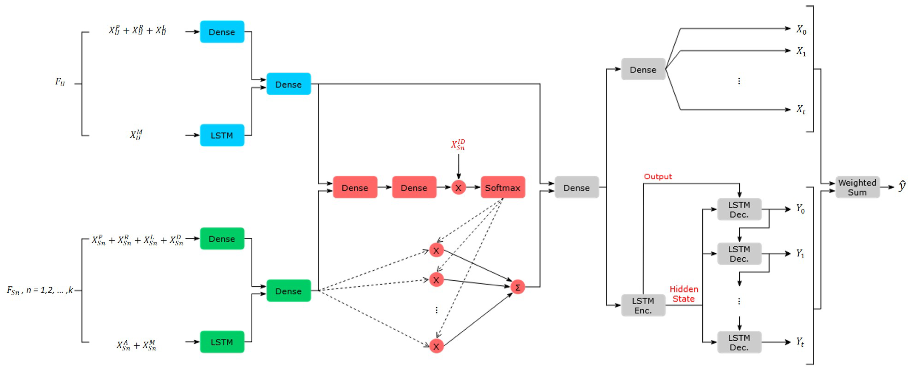
4.2. Feature Extractor

We first introduce the feature extractor, which is the input layer of our model. The input layer consists of two independent feature extractors that process the unlabeled grid $G_U$ and labeled grids $G_S$ separately due to the dimensional difference between the input features. Moreover, the input features are composed of non-sequential data and sequential data. Thus, we extract their embedding vectors separately in different ways.

Since the input features, air quality index $X^A$ and meteorological features $X^M$ are long-term time-related, we can use recurrent neural network (RNN) to encode each of the sequential features. Although RNN is designed to deal with time series data, this technique suffers from a vanishing or exploding gradient problem. To deal with the flaws, long short-term memory (LSTM) is proposed in [23]. In Equation (2), the first two gates control the proportion of previous state $C_{(t-1)}$ and generate the current state $C_t$. Then, the output gate is used to control the amount of cell states to generate the current output value $h_t$.

$$\begin{array}{c}{i}_t=\sigma (W_i[X_t,h_{t-1}]+b_i),\\ f_t=\sigma (W_f[X_t,h_{t-1}]+b_f),\\ o_t=\sigma (W_o[X_t,h_{t-1}]+b_o),\\ c_t=f_t\odot c_{t-1}+i_t\odot tanh(W_c[X_t,h_{t-1}]+b_c),\\ h_t=o_t\odot tanh\left(c_t\right),\end{array}$$

(2)

where $W_i$, $W_f$, $W_o$, and $W_c$ are the weights for concatenated input vectors at time step t for each gate, $i_t$ is the input gate’s activation vector, $f_t$ is the forget gate’s activation vector, $o_t$ is the output gate’s activation vector, and $b_i$, $b_f$, $b_o$, and $b_c$ are the biases vectors. To make the model nonlinear, $\sigma$ and $tanh$ are applied as activation functions and ⊙ is the element-wise multiplication of the matrix.

Other static features such as $X^P$, $X^R$, $X^L$ and $X^D$ are non-dynamic related. We employ a single dense layer (the first dense layer in Figure 1a) to extract and learn the interaction between static features.

Then we calculate the static embedding in Equation (3):

$$\begin{array}{c}{e}_U^1=ReLU(W_U^1(X_U^P\oplus X_U^R\oplus X_U^L)+b_U^1),\\ e_{Sn}^1=ReLU(W_S^1(X_{Sn}^P\oplus X_{Sn}^R\oplus X_{Sn}^L\oplus X_{Sn}^D)+b_S^1),\mathrm{for}n=1,\dots ,k\end{array}$$

(3)

where $e_U^1$ and $e_{Sn}^1$ are the output of the first dense layer of unlabeled grids and labeled grids, ⊕ denotes the operation of feature concatenation, and rectified linear unit (ReLU) is our activation function. After extracting both static features and sequential features, we aim to capture the correlation between them. We further construct another dense layer on top of LSTM and the first dense layer, in order to obtain the feature interaction and calculate the embedding feature of each grid. We can have an interactive dense layer in Equation (4):

$$\begin{array}{c}{e}_U^2=ReLU(W_U^2(e_U^1\oplus h_U^t)+b_U^2),\\ e_{Sn}^2=ReLU(W_S^2(e_{Sn}^1\oplus h_{Sn}^t)+b_S^2),\mathrm{for}n=1,\dots ,k\end{array}$$

(4)

in which $e_U^2$ and $e_{Sn}^2$ are the outputs of the feature extractor for unlabeled grids and labeled grids, and $h^t$ is the last hidden state of LSTM. In Equation (4), we use the same weight and bias in the feature extractor for all k labeled grids. Since the labeled grids are the same, learning shared weight is a method to reduce duplicated computation and parameter numbers.

4.3. Inversed Distance Attention

The proposed inversed distance attention is shown in Figure 1b. We can acquire the spatio-temporal embedding vectors of unlabeled grids and all labeled grids through the first layer feature extractor. However, not all labeled grids have the same contribution to each unlabeled grid. The attention mechanism [24] is a beneficial structure that computes their different contributions. Hence, we apply the attention technique in our model to learn the importance between unlabeled grids and all labeled grids. There are a total of k embedding vectors of labeled grids. Generally, attention networks calculate the attention score of two vectors: $e_U^2$ and $e_{Sn}^2$ for k times. Then we exploit each attention score as the pooling coefficient to multiply $e_{Sn}^2$ and sum up the results of all grids as one embedding vector.

Inner product, cosine similarity, and multilayer perceptron (MLP) are common methods to calculate the attention score. In our model, we make use of MLP as the base attention network because its performance is the best of common methods. In Equation (5), we first concatenate $e_U^2$ and $e_{Sn}^2$ and use two dense layers as MLP attention mechanism to obtain the correlation values.

$$\begin{array}{c}{e}_{ATTn}=ReLU(W_{ATT}^2\left(ReLU(W_{ATT}^1(e_U^2\oplus e_{Sn}^2)+b_{ATT}^1)\right)+b_{ATT}^2),\mathrm{for}n=1,\dots ,k\end{array}$$

(5)

$$\begin{array}{c}{a}_{Sn}=\frac{exp(e_{ATTn}\ast X_{Sn}^{ID})}{{\sum }_{n=1}^{k}exp(e_{ATTn}\ast X_{Sn}^{ID}))},\mathrm{for}n=1,\dots ,k\end{array}$$

(6)

$$\begin{array}{c}{e}_S^3=\sum _{n=1}^k{e}_{Sn}^2\times a_{Sn}\end{array}$$

(7)

Generally, the attention score can be obtained by directly encoding all correlation values by softmax layer. However, the distance between $G_U$ and $G_{Sn}$ might have a high influence when calculating the correlation. It is conceivable that the closer to $G_U$ in $G_{Sn}$, the more impact there will be on $G_U$, so in Equation (6) we multiply the inversed distance feature ($X_{Sn}^{ID}$) and correlation values before the softmax layer. We can have an attention score for each labeled grid after the softmax layer, and use them as a weighted coefficient to obtain the final output $e_S^3$ of inversed distance attention in Equation (7).

4.4. Hybrid Predictor

In this section, we detail our proposed structure for prediction. The main purpose of the prediction layer in Figure 1c is to obtain the predicted AQI values from the final embedding vector. First, the final embedding vector is obtained by concatenating the output of the inversed distance attention ($e_S^3$) and the embedding vector of unlabeled grids ($e_U^2$). Although our predicted target can be taken as a regression problem, we can use MLP to process embedding vectors and predict the results. Compared to the common regression problem, directly using traditional MLP does not yield good accuracy, due to the lack of historical AQI data from unlabeled grids. Therefore, we propose a hybrid predictor to solve the problem and achieve a better long-term prediction by splitting the predicted values into two data flows. We assume that predicted values can be separated into two independent fractions: time-independent and time-dependent. We design two divided predictor structures that have two independent data flows to predict the AQI, respectively. In the end of the predictor, we sum the predicted values up with dynamic weights to combine these two data flows on each prediction timestamp.

We apply the first dense layer behind the inversed distance attention layer to learn the cross features of unlabeled grid embedding and attention output. In Equation (8), we can have a cross embedding vector ($e_Z$) for the prediction of two data flows after the dense layer.

$$\begin{array}{c}{e}_Z=ReLU(W_Z(e_U^2\oplus e_S^3)+b_Z)\end{array}$$

(8)

We then directly use MLP, a common method for a regression problem, to predict one data flow. As Equation (9), we can have time-independent predicted values for future time t by using an additional dense layer.

$$\begin{array}{c}{X}_m=W_x{e}_Z+b_x,\mathrm{for}m=0,1,\dots ,t\end{array}$$

(9)

Another predicted data flow, time-dependent flow, means the prediction for the next timestamp is based on the current prediction and so on for further timestamp prediction. To achieve this goal, we propose an LSTM predictor that is based on the structure of LSTM AutoEncoder [25]. AutoEncoder is a common unsupervised learning method that usually trains a hidden embedding vector for the image, or compresses the dimension of vectors. AutoEncoder is a structure that minimizes the error between input and output vectors. We use the concept of the decoder part for time-dependent data flow in our model.

LSTM Enc. refers to the structure of LSTM Encoder in Figure 2. Because the input of LSTM should be a sequence, we repeat the cross embedding vector ($e_Z$) several times as a sequence input. Through the processing of the encoder, we can have output ($e_{Enc.}$) and hidden state $(h_t^{AE},c_t^{AE})$ of the encoder for the next step in Equations (10) and (11).

$$\begin{array}{c}{e}_{LSTM},(h_t^{AE},c_t^{AE})=LSTMEnc.\left(e_Z\right)\end{array}$$

(10)

$$\begin{array}{c}{e}_{Enc.}=ReLU\left(e_{LSTM}\right)\end{array}$$

(11)

LSTM Dec. in Figure 2 is composed of one LSTM and one dense layer. We have a total of t LSTM decoders which have the same hidden sizes as the t number of the encoder’s LSTM. In Equation (12), we take the output of the encoder that usually represents the last layer of $h_t^{AE}$ as the initial input of the decoder. The hidden state of the encoder is also the initial hidden state for all decoder units. In other words, we set the same hidden state for both the encoder and all decoders in back-propagation. Meanwhile, in Equation (13), the output of the first decoder would be the input of the second decoder, and so on until t time periods. With our proposed LSTM predictor, the data flow of time-dependent prediction can be dealt with.

$$\begin{array}{c}{Y}_0=LSTMDec.(e_{Enc},(h_t^{AE},c_t^{AE}))\end{array}$$

(12)

$$\begin{array}{c}{Y}_m=LSTMDec.(Y_{m-1},(h_t^{AE},c_t^{AE})),\mathrm{for}m=1,2,\dots ,t\end{array}$$

(13)

From two separate predicting data flows, we acquire two complementary predicted values that are time-independent, as well as time-dependent values for the future t time periods. Then we aggregate the results of the two data flows. Although it is intuitive to simply sum the two components to obtain final predicted values, we should also take into account that the proportion of two components is not equal in all timestamps. Hence, we exploit the dynamic weights sum to yield results $\widehat{y}$ in Equation (14):

$$\begin{array}{c}\widehat{y}=\sum _{m=0}^t({\alpha }_m\ast X_m+{\beta }_m\ast Y_m)\end{array}$$

(14)

in which ${\alpha }_t$ is the weight of time-independent predictor and ${\beta }_t$ is the weight of time dependent on predicted time t. We do not define ${\alpha }_t$ and ${\beta }_t$ as fixed values but use them as dynamic weights to learn the proportions automatically in all timestamps during the training processing. A better performance can be achieved by our proposed dynamic weights summation method. In Figure 2, we illustrate our technical data flows and the components of the proposed framework.

5. Experiments

In this section, we first introduce the Beijing dataset used in this study. Then, we include the details of the experimental setting. Finally, we present the experimental results.

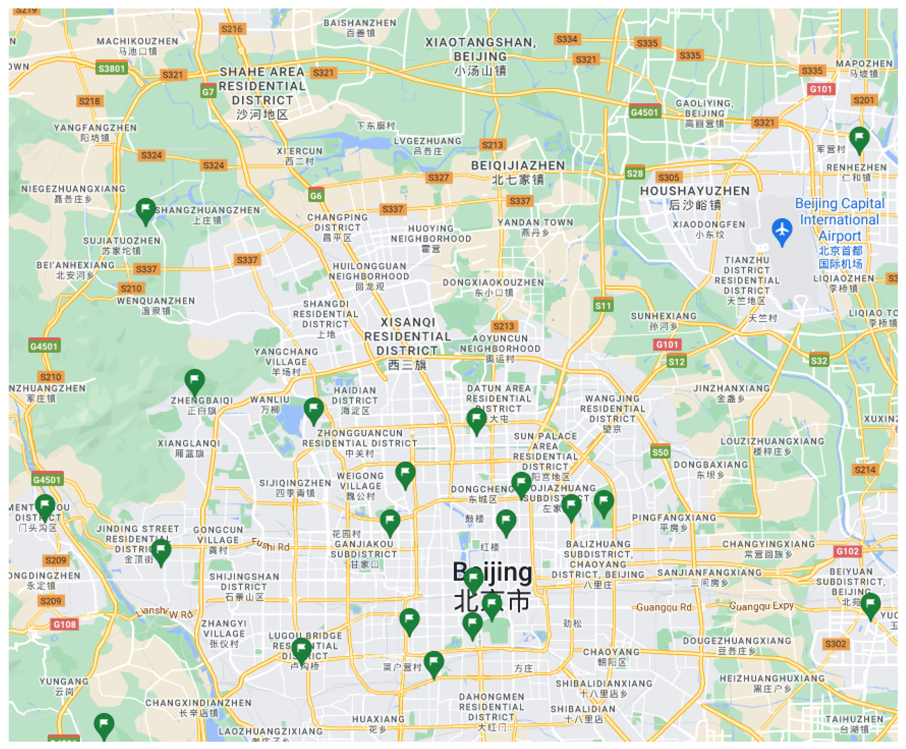
5.1. Dataset

In this study, we set ${115.9}^{\circ }$ E∼${117.2}^{\circ }$ E and ${39.38}^{\circ }$ N∼${40.6}^{\circ }$ N as our target region. We then divided the target region into a total of 3172 grids with a resolution of approximately 2.2 km × 2.2 km (${0.025}^{\circ }$ longitude and ${0.02}^{\circ }$ latitude.) In addition, we made sure there was no more than one station in a grid. Figure 3 shows the target region, where each green mark represents the location of a certain monitoring station. In total, there are 35 monitoring stations in the target region.

The input features of the models include the AQI, meteorological data, POIs, road networks, and land use. These features were collected from 1 January 2017 to 31 December 2017 hourly. Notably, we have the historical PM_2.5 data of all monitoring stations, and fine-grained meteorological records of the target location for all experiments.

5.2. Experimental Settings and Evaluation Metrics

Because the fine-grained air quality data were unavailable, we selected some monitoring stations as unlabeled locations and the predicted targets. Specifically, in the total 35 grids with monitoring stations, we randomly selected 15 grids as labeled grids $G_{Sn}$ and the rest of grids as unlabeled grids $G_{Un}$. We used all 8760 timestamps in a year to collect valid input data and predicted values for training and testing. All available data are partitioned into a training set, validation set, and testing set at an 8:1:1 ratio. Figure 4 is an example with k monitoring stations selected as labeled grids, and the current time is Tc. According to the problem definition in Section 3, we take Tc − 23 PM_2.5 data of labeled grids as input features and Tc + 24 PM_2.5 data of remaining unlabeled grids as a single piece of available data. In other words, the total number of all remaining unlabeled grids is the number of valid instances in time Tc (monitoring sensors sometimes have missing values). To obtain sufficient training and testing data, it is impossible to ensure that all timestamps in all k selected stations have complete historical data. Therefore, we made sure that at least one unlabeled grid will not have missing data in the future. We looked over all timestamps to collect available data and set k as 15 to calculate the amount of all available data in our experiment.

The mean absolute error (MAE) and the root mean square error (RMSE) are used as the evaluation metrics to evaluate the predicted and the ground truth air quality value. The definitions of MAE and RMSE are as follows:

$$\begin{array}{c}MAE=\frac{1}{n}\sum _{i=1}^n|\widehat{y}-y|\end{array}$$

(15)

$$\begin{array}{c}RMSE=\sqrt{\frac{1}{n}{\sum }_{i=1}^n{(\widehat{y}-y)}^2}\end{array}$$

(16)

where $\widehat{y}$ and y are the predicted and observed ground truth values, respectively. We calculated average MAE and RMSE for the current time (0 h) and the future times (1–6, 7–12, 13–18, and 19–24 h).

In order to obtain robust evaluation results, we ran the experiment 10 times and used the average MAE and RMSE scores as representative. In each run, we randomly selected labeled and unlabeled grids and made sure that the combinations of monitoring stations selections were different from the previous runs.

5.3. Experimental Results

First, we show the performance comparison between our model and some baseline methods. Then, we discuss how different numbers of labeled grids affect performance. Finally, we conduct the ablation studies to show the advantages of the proposed inversed distance attention and hybrid predictor.

5.3.1. Comparison with Baseline Models

Baseline models can be divided into two categories, non-NN-based methods and NN-based methods. The non-NN-based methods include K-nearest neighbor (K-NN), weighted K-NN, GBDT regression, and linear regression. The NN-based methods include MLP, LSTM, and LSTM-IDW. The details of the baseline models are as follows.

• K-nearest neighbor (K-NN) regression: The idea of the K-NN regressor is to predict the value by using the nearest monitoring stations as references. In this study, we set the nearest neighbors to three (i.e., k = 3). That is, the predicted value was calculated by using the average scores of the three nearest stations.
• Weighted KNN regression: The weighted K-NN predicts the target values by using the inverse-distance-weighted [26] average scores of the nearest stations. That is, a closer station will have a greater influence on the predicted value of the target station. In this study, we used k = 3 as the setting of the K-NN regressor.
• Gradient Boosting Decision Tree (GBDT) regression: GBDT is a state-of-art tree-based model that captures complex cross features [27].
• Linear Regression: A linear model that assumes a linear relationship between the input variables and the output variable.

• Multilayer Perceptron (MLP): For the MLP model, we concatenate all features on all timestamps as input. The MLP model has two layers.
• LSTM: For the LSTM model, we concatenated all static features with every time step of time-series data as input features. The LSTM model contains two LSTM layers and one dense output layer.
• LSTM-IDW: The LSTM-IDW model is a combination of the LSTM model and the IDW method. We use LSTM to make an AQI prediction of the labeled grids using their historical data first, and then use IDW interpolation to infer the future predictive values of unlabeled grids based on the prediction values of LSTM.

Table 1. Comparison between the proposed and the baseline models. The values in the table are the MAE and RMSE of AQI values.

Methods	Metrics	${\mathit{T}}_{\mathbf{0}}$	${\mathit{T}}_{\mathbf{1}}-{\mathit{T}}_{\mathbf{6}}$	${\mathit{T}}_{\mathbf{7}}-{\mathit{T}}_{\mathbf{12}}$	${\mathit{T}}_{\mathbf{13}}-{\mathit{T}}_{\mathbf{18}}$	${\mathit{T}}_{\mathbf{19}}-{\mathit{T}}_{\mathbf{24}}$
k-NN Nearest Average	MAE RMSE	23.19 40.87	32.01 52.82	45.21 71.41	53.25 81.46	58.05 85.92
IDW Interpolation	MAE RMSE	22.80 40.24	31.77 52.44	45.08 71.25	53.43 81.33	57.94 85.78
GBDT Regression	MAE RMSE	21.41 37.33	25.70 41.32	29.90 45.90	32.54 49.83	34.04 51.10
Linear Regression	MAE RMSE	24.93 39.15	29.00 43.68	35.14 51.42	39.09 57.14	40.30 58.38
MLP	MAE RMSE	24.95 43.28	26.64 45.22	31.54 52.23	33.74 56.89	36.02 59.91
LSTM	MAE RMSE	52.66 88.60	53.73 91.33	57.30 97.18	60.90 102.53	62.53 103.55
LSTM-IDW	MAE RMSE	22.80 40.24	31.87 52.61	42.43 68.72	51.29 77.48	57.85 81.22
Our Model	MAE RMSE	19.35 33.78	19.41 32.08	19.72 33.14	20.41 35.88	22.25 39.95

is the overall comparison between baseline models and our proposed model. Our model outperforms baselines particularly in long-term prediction. The results of LSTM-based models are worse than other methods, for the reason that is also the challenge of our target: the lack of historical air quality data of unlabeled grids makes it difficult for LSTM to make predictions.

In addition, the error of LSTM-IDW is slightly smaller than IDW and K-NN, and LSTM-IDW performs much better than LSTM. LSTM-IDW is mostly affected by the accuracy of the first stage predicted method before interpolation, and the limitation of IDW interpolation’s calculating spatial correlation still influences the overall performance. From the results, our proposed model is able to calculate more critical spatial-temporal correlations and performs better than comparative baselines with the same input features.

5.3.2. Ablation Study of Inversed Distance Attention

We used the attention mechanism to calculate the correlation between target prediction regions and grids with monitoring stations. By multiplying the inversed distance feature as a modification term before the softmax layer, the performance of our model will be improved. In this section, we show an ablation analysis with the attention mechanism and the influence of the inversed distance feature. Here we introduce three models for comparison:

• Model without Attention mechanism: We disabled all the attention structures in our model and used summation to aggregate the embedding vectors of all labeled grids.
• Model without Inversed Distance Attention: In Figure 1b, we only disregard the inversed distance feature $X_{Sn}^{ID}$ to calculate the attention weight, while the process and parameter settings are the same as our proposed method.
• Model with Inversed Distance Attention: This is our proposed model with inversed distance attention structure. We compare our prediction result with the two above models to show the advantage of the proposed inversed distance attention layer.

The overall results for inversed distance attention are shown in

Table 2. Ablation analysis on Inversed Distance Attention (IDA) networks. The values in the table are the MAE and RMSE of AQI values.

Methods	Metrics	${\mathit{T}}_{\mathbf{0}}$	${\mathit{T}}_{\mathbf{1}}-{\mathit{T}}_{\mathbf{6}}$	${\mathit{T}}_{\mathbf{7}}-{\mathit{T}}_{\mathbf{12}}$	${\mathit{T}}_{\mathbf{13}}-{\mathit{T}}_{\mathbf{18}}$	${\mathit{T}}_{\mathbf{19}}-{\mathit{T}}_{\mathbf{24}}$
Without Attention	MAE RMSE	21.53 36.74	20.88 35.40	22.00 37.35	22.12 39.94	24.91 45.75
Without IDA	MAE RMSE	20.42 33.28	19.67 31.84	20.68 33.26	21.21 36.12	23.14 40.65
With IDA	MAE RMSE	19.35 33.78	19.41 32.08	19.72 33.14	20.41 35.88	22.25 39.95

. In the first and second rows, a simple attention layer can improve the performance by giving the high influential grids critical weights. Moreover, in the second and third rows, we prove that multiplying the inversed distance before the softmax layer can further decrease errors. Thus, the distances between unlabeled grids and labeled grids can significantly impact the finding of related reference grids with monitoring stations.

5.3.3. Ablation Study of Hybrid Predictor

We study the advantages of our hybrid predictor in this section. Hence, we test our proposed hybrid predictor with the ablation analysis and verify whether our overall framework can achieve the best performance. First, we compare our performance with different individual predictors. The first one is MLP as the time-independent predictor, and the second one is the LSTM AutoEncoder as the time-dependent predictor. Namely, we divide our framework into two data flows to predict the result separately in this experiment. Second, we combine these two predictors into a hybrid predictor as a testing model with a simple sum. We sum up the results of two predictors with equal weight. Finally, we use the proposed dynamic weights sum to aggregate the results and compare them to the results of the summation that has no dynamic weights sum. In this part, we show our proposed idea step by step with the results.

However, we expect a prediction model might have better performance during the current time than the more extended periods. That is to say, the trend of the error from $T_0$ to $T_{19-24}$ should be incremental, meeting our expectations for real life. From

Table 3. The MAE with only MLP as the predictor for all 10 times. The values in the table are the MAE of AQI values.

No. of Data	${\mathit{T}}_{\mathbf{0}}$	${\mathit{T}}_{\mathbf{1}}-{\mathit{T}}_{\mathbf{6}}$	${\mathit{T}}_{\mathbf{7}}-{\mathit{T}}_{\mathbf{12}}$	${\mathit{T}}_{\mathbf{13}}-{\mathit{T}}_{\mathbf{18}}$	${\mathit{T}}_{\mathbf{19}}-{\mathit{T}}_{\mathbf{24}}$
Data 1	18.53	18.50	20.79	19.82	21.85
Data 2	22.11	20.14	19.23	19.09	20.30
Data 3	24.41	22.54	23.63	23.40	29.16
Data 4	17.88	18.31	18.90	20.48	23.59
Data 5	18.68	21.77	26.85	22.76	24.47
Data 6	23.28	19.83	22.08	23.17	25.53
Data 7	23.80	23.19	25.07	23.80	24.80
Data 8	22.13	19.76	19.97	23.97	23.45
Data 9	19.81	17.73	18.78	20.05	21.54
Data 10	18.02	17.61	18.79	19.39	22.16
AVERAGE	20.86	19.94	21.41	21.59	23.68

and

Table 4. The MAE with only LSTM AutoEncoder as the predictor for all 10 times. The values in the table are the MAE of AQI values.

No. of Data	${\mathit{T}}_{\mathbf{0}}$	${\mathit{T}}_{\mathbf{1}}-{\mathit{T}}_{\mathbf{6}}$	${\mathit{T}}_{\mathbf{7}}-{\mathit{T}}_{\mathbf{12}}$	${\mathit{T}}_{\mathbf{13}}-{\mathit{T}}_{\mathbf{18}}$	${\mathit{T}}_{\mathbf{19}}-{\mathit{T}}_{\mathbf{24}}$
Data 1	25.41	25.59	28.45	31.00	33.14
Data 2	31.70	27.86	25.01	26.77	32.33
Data 3	28.73	29.01	31.15	34.45	43.32
Data 4	27.00	28.76	30.65	34.68	37.84
Data 5	25.52	27.91	33.87	33.67	34.52
Data 6	28.28	27.64	31.20	33.95	37.78
Data 7	30.75	30.88	30.54	29.28	29.05
Data 8	33.25	31.23	34.69	39.48	42.04
Data 9	28.00	26.77	27.81	28.80	32.11
Data 10	22.77	22.97	25.32	25.77	29.80
AVERAGE	28.14	27.86	29.87	31.78	35.19

, we only show the results with MAE to compare each predictor, since the trends of MAE and RMSE are similar. We list all 10 experiment results simultaneously for a more detailed comparison between two different predictors.

The results with the MLP predictor (Table 3) are obviously superior in that the overall MAE is better than the results with the LSTM AutoEncoder predictor (Table 4), whether in every experiment or the average results. However, the accuracy trend of the LSTM AutoEncoder predictor is more realistic than the MLP predictor. We mark the values in $T_0$ that are worse than $T_{1-6}$ in Table 3 and Table 4 and denote them as unexpected $T_0$, and find that the number of unexpected $T_0$ in Table 3 is more than in Table 4. Thus, we can have a hypothesis that each predictor structure has its advantages and disadvantages, and their combined effectiveness proves that their results are complementary.

Hence, the aggregation of two data flows shows that the two predictors are complementary and beneficial to our proposed method.

Table 5. The results of aggregating two data flow with simple summation in all 10 times. The values in the table are the MAE of AQI values.

No. of Data		${\mathit{T}}_{\mathbf{0}}$	${\mathit{T}}_{\mathbf{1}}-{\mathit{T}}_{\mathbf{6}}$	${\mathit{T}}_{\mathbf{7}}-{\mathit{T}}_{\mathbf{12}}$	${\mathit{T}}_{\mathbf{13}}-{\mathit{T}}_{\mathbf{18}}$	${\mathit{T}}_{\mathbf{19}}-{\mathit{T}}_{\mathbf{24}}$
Data 1		16.88	17.31	18.39	19.66	20.61
Data 2		20.46	17.90	17.46	18.80	19.83
Data 3		23.12	20.86	22.39	23.74	28.83
Data 4		17.50	19.16	19.37	21.29	23.29
Data 5		18.60	21.90	26.15	22.00	25.08
Data 6		20.28	18.33	20.41	21.31	23.84
Data 7		21.40	22.67	24.79	23.46	24.08
Data 8		23.41	20.61	19.24	22.27	23.29
Data 9		20.17	17.76	18.72	19.71	20.22
Data 10		15.42	15.93	17.16	17.41	18.78
AVERAGE	MAE RMSE	19.72 33.90	19.24 32.76	20.41 34.76	20.97 37.46	22.78 41.71

shows the result from integrating two predictors by simply adding up. Through simple summation, the overall MAE is better than with each predictor individually, and the number of unexpected $T_0$ is less than the results in Table 3. Thus, we easily confirm that a simple sum hybrid predictor can enhance the performance and that separating the predicted values into two independent data flows is effective.

Last but not least, we assume that the proportions of the MLP predictor and LSTM AutoEncoder predictor might not be the same for all cases. Hence, we propose to sum up the dynamic weights in our model and show the results in

Table 6. The detailed results of our proposed model with weighted summation for all 10 times. The values in the table are the MAE of AQI values.

No. of Data		${\mathit{T}}_{\mathbf{0}}$	${\mathit{T}}_{\mathbf{1}}-{\mathit{T}}_{\mathbf{6}}$	${\mathit{T}}_{\mathbf{7}}-{\mathit{T}}_{\mathbf{12}}$	${\mathit{T}}_{\mathbf{13}}-{\mathit{T}}_{\mathbf{18}}$	${\mathit{T}}_{\mathbf{19}}-{\mathit{T}}_{\mathbf{24}}$
Data 1		16.92	17.49	18.78	19.36	20.18
Data 2		19.98	18.24	18.38	18.83	19.93
Data 3		21.02	20.17	20.31	21.11	22.26
Data 4		19.86	22.63	23.77	24.89	30.67
Data 5		16.18	18.15	18.33	17.83	19.18
Data 6		20.92	20.83	19.16	20.93	23.08
Data 7		21.96	22.36	23.81	22.97	25.89
Data 8		22.34	20.78	20.34	23.52	23.80
Data 9		19.16	17.49	17.54	17.92	19.34
Data 10		15.21	15.98	16.76	16.75	18.17
AVERAGE	MAE RMSE	19.35 33.78	19.41 32.08	19.72 33.14	20.41 35.88	22.25 39.95

. We exploit the MAE of 10 groups data and the overall MAE and RMSE to compare the difference between simple sum in Table 5 and dynamic weights sum in Table 6. Even though the number of unexpected $T_0$ is the same, the overall MAE and RMSE have both improved with the dynamic weights sum. In conclusion, our proposed hybrid predictor with dynamic weights sum efficiently reduces overall errors and can meet the demand in real life as well.

5.3.4. Affection of Number of Labeled Grids

Generally, errors are fewer when more labeled grids are selected. Missing observed values in a real case is usual. Hence, in our experimental settings in Section 5.2, the number of labeled grids might influence available data for training and testing. In other words, it is more difficult to have complete historical PM_2.5 data with at least 20 labeled grids than with at least 15 labeled grids. In this part, we experiment with the different numbers of labeled grids (k) to discuss the effect of k.

To set up the experiment, we select the same amount (15,210) of data with different k. Namely, k as the only variation means that the result will not be influenced by the total amount of data or predicted target. We experiment with k at 10, 15, and 20 as appropriate values in our dataset. First, we randomly select 20 labeled grids from 35 grids with monitoring stations and collect all available data. Next, we randomly select 15 grids from the previously selected 20 as the labeled grids and with k = 15, and randomly select 10 from the selected 15 grids. We then filter the selected number of k stations in previously collected data. The predicted unlabeled grids, predicted values and the number of all collected available data are the same with a different k. The only difference is the set of labeled grids used for reference. We then repeat the steps to select grids and collect available data 10 times and also evaluate the effect of k with average MAE and RMSE in

Table 7. Comparison results for our proposed model with the different number k of labeled grids. The values in the table are the MAE and RMSE of AQI values.

Number of Labeled Grids (k)	Metrics	${\mathit{T}}_{\mathbf{0}}$	${\mathit{T}}_{\mathbf{1}}-{\mathit{T}}_{\mathbf{6}}$	${\mathit{T}}_{\mathbf{7}}-{\mathit{T}}_{\mathbf{12}}$	${\mathit{T}}_{\mathbf{13}}-{\mathit{T}}_{\mathbf{18}}$	${\mathit{T}}_{\mathbf{19}}-{\mathit{T}}_{\mathbf{24}}$
k = 10	MAE RMSE	20.89 36.71	23.22 40.73	27.94 47.36	27.76 47.34	32.22 56.61
k = 15	MAE RMSE	19.98 35.86	22.62 39.74	27.46 45.67	26.63 44.94	30.43 52.54
k = 20	MAE RMSE	19.43 35.01	21.83 39.05	25.72 43.63	25.33 42.59	28.8 50.33

. As we expected, our model performs better with a larger k because there is more referable monitoring stations. However, a larger k is not feasible in real life due to the completeness of observed data stated in the previous section. Thus, we choose an appropriate k = 15 as our setting in this dataset.

6. Conclusions

In this study, we propose a new topic in air quality prediction that forecasts the fine-grained air quality in regions without monitoring stations. The challenge to this objective is the lack of historical air quality data, which is crucial to precise long-term prediction. Hence, we propose a hybrid predictor structure that consists of two data flows to predict time-independent and time-dependent values respectively. We then combine the two complementary results with the dynamic weights sum, which effectively increases the accuracy of long-term prediction. Additionally, we propose inversed distance attention based on the MLP attention mechanism that further improves the overall performance. Our attention networks can provide crucial correlation information of all monitoring stations, as well as any region in the city for an accurate fine-grained air quality prediction. According to the experiment results, our model outperforms all baselines significantly for the next 19–24 h in MAE and RMSE. As a result, our fine-grained air quality prediction not only performs well in the current time but satisfies the demand for long-term prediction. In our future plan, we aim to devise a score specific to the air quality prediction problem that quantifies the human health improvement induced by the model to measure the model prediction performance.

References

- Xing, Y.F.; Xu, Y.H.; Shi, M.H.; Lian, Y.X. The impact of PM2.5 on the human respiratory system. J. Thorac. Dis. 2016, 8, E69. [Google Scholar] [PubMed]
- Menut, L.; Bessagnet, B.; Siour, G.; Mailler, S.; Pennel, R.; Cholakian, A. Impact of lockdown measures to combat Covid-19 on air quality over western Europe. Sci. Total Environ. 2020, 741, 140426. [Google Scholar] [CrossRef] [PubMed]
- Qin, S.; Liu, F.; Wang, C.; Song, Y.; Qu, J. Spatial-temporal analysis and projection of extreme particulate matter (PM10 and PM2.5) levels using association rules: A case study of the Jing-Jin-Ji region, China. Atmos. Environ. 2015, 120, 339–350. [Google Scholar] [CrossRef]
- Zheng, Y.; Yi, X.; Li, M.; Li, R.; Shan, Z.; Chang, E.; Li, T. Forecasting fine-grained air quality based on big data. In Proceedings of the 21th ACM SIGKDD International Conference on Knowledge Discovery and Data Mining, Sydney, Australia, 10–13 August 2015; pp. 2267–2276. [Google Scholar]
- Hsieh, H.P.; Lin, S.D.; Zheng, Y. Inferring air quality for station location recommendation based on urban big data. In Proceedings of the 21th ACM SIGKDD International Conference on Knowledge Discovery and Data Mining, Sydney, Australia, 10–13 August 2015; pp. 437–446. [Google Scholar]
- Le, V.D.; Bui, T.C.; Cha, S.K. Spatiotemporal deep learning model for citywide air pollution interpolation and prediction. In Proceedings of the 2020 IEEE International Conference on Big Data and Smart Computing (BigComp), Busan, Korea, 19–22 February 2020; IEEE: Piscataway, NJ, USA; pp. 55–62. [Google Scholar]
- Kumar, K.; Yadav, A.; Singh, M.; Hassan, H.; Jain, V. Forecasting daily maximum surface ozone concentrations in Brunei Darussalam—An ARIMA modeling approach. J. Air Waste Manag. Assoc. 2004, 54, 809–814. [Google Scholar] [CrossRef] [PubMed] [Green Version]
- Lateb, M.; Meroney, R.N.; Yataghene, M.; Fellouah, H.; Saleh, F.; Boufadel, M. On the use of numerical modelling for near-field pollutant dispersion in urban environments—A review. Environ. Pollut. 2016, 208, 271–283. [Google Scholar] [CrossRef] [PubMed] [Green Version]
- Rybarczyk, Y.; Zalakeviciute, R. Machine learning approaches for outdoor air quality modelling: A systematic review. Appl. Sci. 2018, 8, 2570. [Google Scholar] [CrossRef] [Green Version]
- Xayasouk, T.; Lee, H.; Lee, G. Air pollution prediction using long short-term memory (LSTM) and deep autoencoder (DAE) models. Sustainability 2020, 12, 2570. [Google Scholar] [CrossRef] [Green Version]
- Zheng, Y.; Liu, F.; Hsieh, H.P. U-air: When urban air quality inference meets big data. In Proceedings of the 19th ACM SIGKDD International Conference on Knowledge Discovery and Data Mining, Chicago, IL, USA, 11–14 August 2013; pp. 1436–1444. [Google Scholar]
- Cheng, W.; Shen, Y.; Zhu, Y.; Huang, L. A neural attention model for urban air quality inference: Learning the weights of monitoring stations. In Proceedings of the Thirty-Second AAAI Conference on Artificial Intelligence, New Orleans, LA, USA, 2–7 February 2018. [Google Scholar]
- Lin, Y.; Mago, N.; Gao, Y.; Li, Y.; Chiang, Y.Y.; Shahabi, C.; Ambite, J.L. Exploiting spatiotemporal patterns for accurate air quality forecasting using deep learning. In Proceedings of the 26th ACM SIGSPATIAL International Conference on Advances in Geographic Information Systems, Seattle, WA, USA, 6–9 November 2018; pp. 359–368. [Google Scholar]
- Chen, L.; Ding, Y.; Lyu, D.; Liu, X.; Long, H. Deep multi-task learning based urban air quality index modelling. Proc. ACM Interact. Mobile Wearable Ubiquitous Technol. 2019, 3, 1–17. [Google Scholar] [CrossRef]
- Qi, Y.; Li, Q.; Karimian, H.; Liu, D. A hybrid model for spatiotemporal forecasting of PM2.5 based on graph convolutional neural network and long short-term memory. Sci. Total Environ. 2019, 664, 1–10. [Google Scholar] [CrossRef] [PubMed]
- Qi, Z.; Wang, T.; Song, G.; Hu, W.; Li, X.; Zhang, Z. Deep air learning: Interpolation, prediction, and feature analysis of fine-grained air quality. IEEE Trans. Knowl. Data Eng. 2018, 30, 2285–2297. [Google Scholar] [CrossRef] [Green Version]
- Soh, P.W.; Chang, J.W.; Huang, J.W. Adaptive deep learning-based air quality prediction model using the most relevant spatial-temporal relations. IEEE Access 2018, 6, 38186–38199. [Google Scholar] [CrossRef]
- Li, L.; Zhang, X.; Holt, J.B.; Tian, J.; Piltner, R. Spatiotemporal interpolation methods for air pollution exposure. In Proceedings of the Ninth Symposium of Abstraction, Reformulation, and Approximation, Catalonia, Spain, 17–18 July 2011. [Google Scholar]
- Wong, D.W.; Yuan, L.; Perlin, S.A. Comparison of spatial interpolation methods for the estimation of air quality data. J. Exp. Sci. Environ. Epidemiol. 2004, 14, 404–415. [Google Scholar] [CrossRef] [Green Version]
- Lin, Y.; Chiang, Y.Y.; Pan, F.; Stripelis, D.; Ambite, J.L.; Eckel, S.P.; Habre, R. Mining public datasets for modeling intra-city PM2.5 concentrations at a fine spatial resolution. In Proceedings of the 25th ACM SIGSPATIAL International Conference on Advances in Geographic Information Systems, Redondo Beach, CA, USA, 7–10 November 2017; pp. 1–10. [Google Scholar]
- Zhao, X.; Xu, T.; Fu, Y.; Chen, E.; Guo, H. Incorporating spatio-temporal smoothness for air quality inference. In Proceedings of the 2017 IEEE International Conference on Data Mining (ICDM), New Orleans, LA, USA, 18–21 November 2017; IEEE: Piscataway, NJ, USA; pp. 1177–1182. [Google Scholar]
- Wang, H. Air Pollution and Meteorological Data in Beijing 2016–2017. 2019. Available online: https://dataverse.harvard.edu/dataset.xhtml?persistentId=doi:10.7910/DVN/RGWV8X (accessed on 10 November 2021).
- Hochreiter, S.; Schmidhuber, J. Long short-term memory. Neural Comput. 1997, 9, 1735–1780. [Google Scholar] [CrossRef] [PubMed]
- Vaswani, A.; Shazeer, N.; Parmar, N.; Uszkoreit, J.; Jones, L.; Gomez, A.N.; Kaiser, Ł.; Polosukhin, I. Attention is All You Need. In Proceedings of the Advances in Neural Information Processing Systems, Long Beach, CA, USA, 4–7 December 2017; pp. 5998–6008. [Google Scholar]
- Srivastava, N.; Mansimov, E.; Salakhudinov, R. Unsupervised learning of video representations using lstms. In Proceedings of the International Conference on Machine Learning. PMLR, Lille, France, 6–11 July 2015; pp. 843–852. [Google Scholar]
- Appice, A.; Ciampi, A.; Fumarola, F.; Malerba, D. Missing sensor data interpolation. In Data Mining Techniques in Sensor Networks; Springer: Berlin/Heidelberg, Germany, 2014; pp. 49–71. [Google Scholar]
- Friedman, J.H. Greedy function approximation: A gradient boosting machine. Ann. Stat. 2001, 29, 1189–1232. [Google Scholar] [CrossRef]