Article

Network Intrusion Detection Model Based on CNN and GRU

1
College of Air and Missile Defense, Air Force Engineering University, Xi’an 710051, China
2
College of Computer, Chang’an University, Xi’an 710061, China
*
Author to whom correspondence should be addressed.
Appl. Sci. 2022, 12(9), 4184; https://doi.org/10.3390/app12094184
Submission received: 3 March 2022 / Revised: 12 April 2022 / Accepted: 18 April 2022 / Published: 21 April 2022
(This article belongs to the Special Issue AI for Cybersecurity)

Abstract

:
A network intrusion detection model that fuses a convolutional neural network and a gated recurrent unit is proposed to address the problems associated with the low accuracy of existing intrusion detection models for the multiple classification of intrusions and low accuracy of class imbalance data detection. In this model, a hybrid sampling algorithm combining Adaptive Synthetic Sampling (ADASYN) and Repeated Edited nearest neighbors (RENN) is used for sample processing to solve the problem of positive and negative sample imbalance in the original dataset. The feature selection is carried out by combining Random Forest algorithm and Pearson correlation analysis to solve the problem of feature redundancy. Then, the spatial features are extracted by using a convolutional neural network, and further extracted by fusing Averagepooling and Maxpooling, using attention mechanism to assign different weights to the features, thus reducing the overhead and improving the model performance. At the same time, a Gated Recurrent Unit (GRU) is used to extract the long-distance dependent information features to achieve comprehensive and effective feature learning. Finally, a softmax function is used for classification. The proposed intrusion detection model is evaluated based on the UNSW_NB15, NSL-KDD, and CIC-IDS2017 datasets, and the experimental results show that the classification accuracy reaches 86.25%, 99.69%, 99.65%, which are 1.95%, 0.47% and 0.12% higher than that of the same type of CNN-GRU, and can solve the problems of low classification accuracy and class imbalance well.

1. Introduction

Network intrusion detection is a security mechanism that has been developed in recent years to dynamically monitor, prevent and defend against system intrusions. It specifically refers to collect information from several nodes of a computer network or system and analyze this information to discover whether there is an attack or a breach of security policy in the network system. Research on intrusion detection technology has been conducted worldwide since the 1980s, and it has now developed into an integral part of the network security architecture [1].
Traditional machine learning methods have been widely used in network intrusion detection systems, such as Bayesian [2,3,4], Support Vector Machines [5,6,7,8,9,10], Decision Trees [11,12,13], Logistic Regression [14,15,16], etc. These methods have achieved good results. However, these methods are not suitable for massive and high-dimensional data, and cannot solve the problem of degraded classification performance due to their own sensitivity to outliers and noise. At the same time, due to the continuous development of digital technology and the increasingly diverse means of cyber-attacks, traditional machine learning methods have had difficulty in meeting the needs of users.
In recent years, deep learning techniques have been widely used in natural language processing [17], image recognition [18] and other fields. These techniques have also achieved good results in the field of intrusion detection by combining low-level features to form a more abstract and non-linear high-level representation, and then mining the input–output relationships between data. The neural networks commonly used in the field of intrusion detection mainly include convolutional neural networks (CNN), recurrent neural networks (RNN), and deep belief networks. In the literature [19], the data traffic is converted into individual pixel points in bytes, and then the images generated from the traffic are fed into convolutional neural network for convolution, pooling and other operations, and finally the classification results are obtained. The method achieves high accuracy in binary classification and multi-classification problems. The literature [20] used the recognized KDD99 dataset to conduct experiments. During the experiments, the Long Short-Term Memory (LSTM) network was used to complete the selection of parameters and achieved more satisfactory experimental results, however, the method resulted in a high false alarm rate due to the improper selection of training parameters. The literature [21] proposed a hierarchical intrusion detection system based on spatial-temporal features, which first uses deep convolutional neural networks to learn low-level spatial features of network traffic, and then uses LSTM to obtain high-level temporal features, however, the method does not consider the problems of feature fusion and data imbalance. The literature [22] combines the features of WaveNet and Bidirectional Gated Recurrent Unit (BiGRU) for feature extraction, and proposes an intrusion detection method that fuses WaveNet and BiGRU. It can achieve better detection accuracy, although it does not consider the problem of sample imbalance.
Although intrusion detection techniques have made great progress, there are also the following problems. First, with regard to feature redundancy, more feature dimensions will not only increase the training time of the model, but also reduce the detection effect of the model. The literature [23] proposed an intrusion detection method based on Principal Component Analysis (PCA) and recurrent neural networks. The principal component analysis method was used to reduce the dimensionality and noise of the data to find out the subset of principal component features containing the maximum information, and then the processed data was trained using RNN networks for classification with a high accuracy rate. The literature [24] proposed an intrusion detection method combining the advantages of an autoencoder and residual network, in which feature extraction was performed by reconstructing the network with an autoencoder, after which the extracted features were used to train the designed residual network, and the experimental results showed good performance in terms of accuracy, true rate and false alarm rate. However, the methods mentioned above in the literature are generally effective in solving the feature redundancy problem. Secondly, the dataset used to evaluate the effectiveness of the model has an unbalanced sample of positive and negative classes. The literature [25] uses an improved local adaptive synthetic minority oversampling technique for unbalanced traffic data to achieve traffic anomaly detection using RNN, which is more accurate for different types of detection, although the improvement is less obvious.
To address the above-mentioned problems, this paper designs an intrusion detection model fusing CNN and GRU. The main contributions are as follows:
(1)
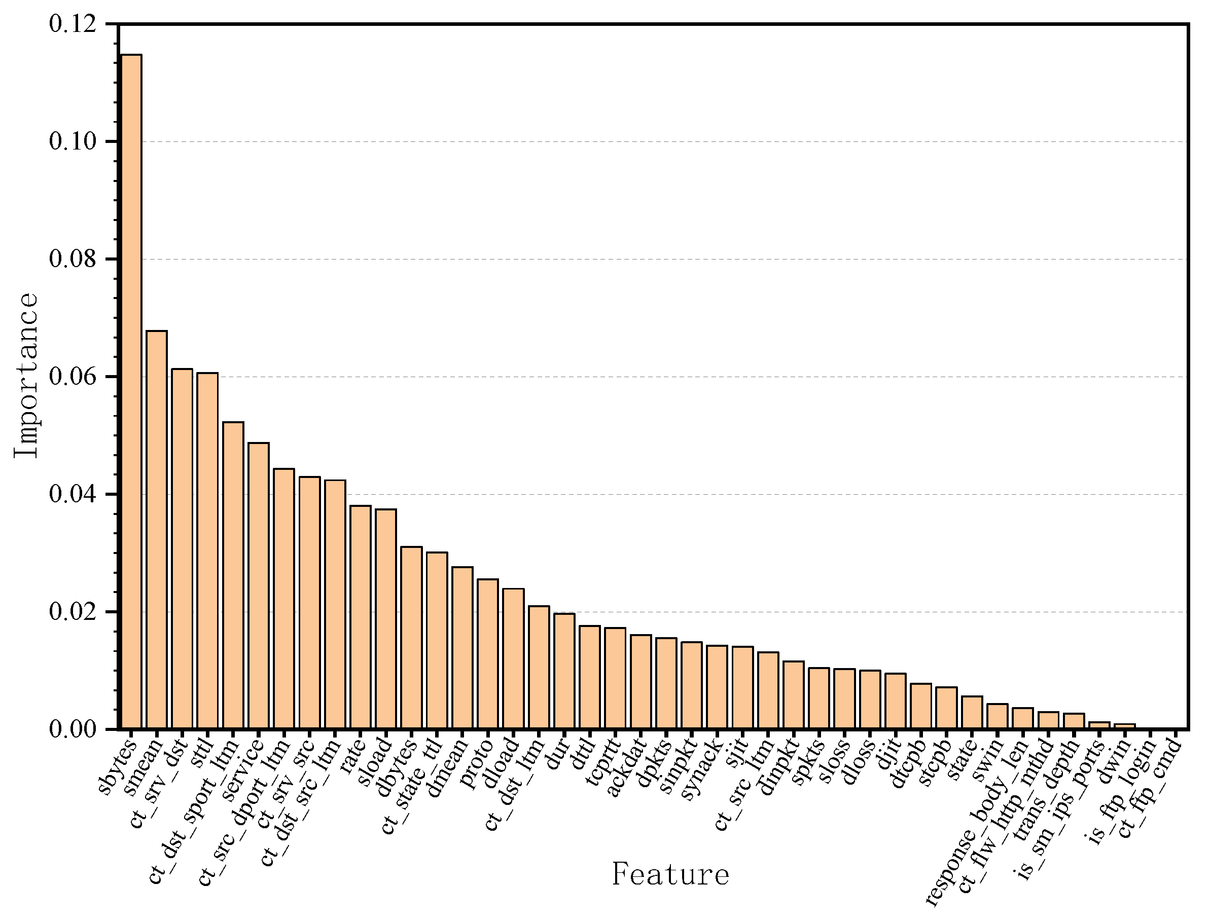
To address the problem of feature redundancy, this paper proposes a feature selection algorithm (RFP algorithm). First, a random forest algorithm is introduced to calculate the importance of features, and then Pearson correlation analysis is used to select features;
(2)
To address the problem of sample imbalance, this paper proposes a hybrid sampling algorithm (ADRDB algorithm) by combining the Adaptive Synthetic Sampling (ADASYN) [26] and Repeated Edited nearest neighbors (RENN) [27] sampling methods for sampling, while using Density-Based Spatial Clustering of Applications with Noise (DBSCAN) [28] to reject noise, and finally achieving a balanced dataset;
(3)
In this paper, CNN is introduced to extract spatial features from the network data traffic and use its weight sharing feature to improve the speed; GRU network is introduced to extract temporal features and learn the dependency between features, so as to avoid overfitting problems; the attention mechanism is introduced to assign different weights to the features, thus reducing the overhead and improving the model performance.

2. Related Work

Network security intrusion detection is a relatively broad area of research. Existing models used in the field of intrusion detection include Convolutional Neural Networks, Recurrent Neural Networks, machine learning, and hybrid models. Scholars have used a variety of different approaches to address the problems of low detection accuracy and difficulty in detecting a few classes of samples in the field of intrusion detection. Convolutional neural networks are primarily used in tasks related to image and video analysis, such as image classification, face recognition, target recognition, image processing and so on. Furthermore, in recent years it has also been widely used in the field of intrusion detection. A recurrent neural network is mainly used in various tasks of connected handwriting recognition and speech recognition. It is also commonly used in the field of intrusion detection due to its effectiveness in processing time series data.
In terms of improving detection accuracy: Tama, B.A. et al. used a combination of particle swarm optimization algorithms, ant colony algorithms and genetic algorithms for feature selection to reduce the feature size of the training data, followed by a secondary classification method to detect abnormal behavior in the network [29]. Bu, S.J. et al. combined a traditional learning classifier system with a convolutional neural network for the detection of anomalous behavior, and the proposed system has adaptive and learning capabilities [30]. Le, T.T.H. et al. first performed feature selection via the SFSDT model, followed by classification via recurrent neural networks, achieving better results on both the NSL-KDD dataset and the ISCX dataset [31]. Hassan, M.M. et al. proposed an intrusion detection system based on CNN and a weight-dropped long short-term memory network, and achieved more satisfactory results [32].
In terms of addressing the class imbalance: Louk, M.H.L. et al. compared existing sampling methods and found that EasyEnsemble performed better in resolving sample imbalance [33]. Liu, L. et al. divided the dataset into hard and easy sets by ENN, and reduced the imbalance of the original dataset by processing the samples in the hard set through the K-Means algorithm [34]. Yan, M. et al. identified anomalous traffic with good accuracy by an improved density peak clustering algorithm [35]. The recent work related to network intrusion detection using optimization algorithms, deep learning algorithms, and machine learning algorithms is given in Table 1.
To effectively select feature subsets and hyperparameters, Abdullah Alharbi et al. [36] proposed a local-global optimal neural network Bat algorithm (LGBA-NN). They tested on the N-BaIoT dataset and compared with several recent advanced methods, such as the particle swarm optimization (PSO) algorithm and Bat algorithm. The experiments demonstrate that the LGBA-NN algorithm has a significant improvement in the detection accuracy of multi-class botnets up to 90%.
Jevgenijus Toldinas et al. [37] first transformed the original network data into four-channel (Red, Green, Blue, and Alpha) images, which were later divided into a training and a testing set. The obtained images were classified based on the ResNet50 model and evaluated on the UNSW_NB15 and BOUN_Ddos datasets. The experimental results demonstrate that the proposed model has a high accuracy in detecting anomalous attacks.
In response to the ongoing and changing malicious threats in the current cyber environment, Muhammad Ashfaq Khan [38] proposes a hybrid intrusion detection system based on deep learning (HRCNNIDS). The authors use convolutional neural networks to capture regional features and temporal features through recurrent neural networks and evaluate the proposed system based on CSE-CIC-IDS2018 dataset. The experimental results show that the method has a high detection rate for malicious attacks.
In recent years, the number and complexity of attacks on network environments have continued to rise, and Guo Pu et al. [39] proposed an unsupervised anomaly detection method for network intrusion detection work. They combined subspace clustering (SSC) and a class of support vector machines (OCSVM) to achieve better performance on the NSL-KDD dataset.
Gia Nhu Nguyen et al. [40] introduced blockchain data transfer technology to the field of intrusion detection to both secure data and improve detection efficiency. Their proposed model uses sensors to collect data, after which intrusion detection is performed through deep belief networks. In addition, the model ensures privacy and security by sharing the created model. The authors evaluated the proposed model through NSL-KDD 2015 and CIDDS-001 datasets and achieved better results.
To address the existing problem of imbalanced intrusion detection data samples, Ranjit Panigrahi et al. [41] proposed a host-based intrusion detection algorithm. They first generate balanced samples from high-level imbalanced datasets in the preprocessing stage by an improved random sampling mechanism. Then the datasets are filtered by an improved multi-class feature selection mechanism. Finally, a merged tree construction algorithm based on the C4.5-based detector is built. The experimental results show that their proposed algorithm achieves a very high detection accuracy.
In their study, MohammadNoor Injadat et al. [42] fully considered the impact of sampling techniques on model performance and compared two feature selection techniques based on information gain and correlation, and finally proposed the multi-stage optimization of an intrusion detection system based on machine learning. In this system, they first sample the dataset by the SMOTE algorithm, followed by feature selection, and finally optimize the parameters of the model by the optimization algorithm. Experiments through evaluation on the UNSW_NB15 dataset and CIC-IDS2017 dataset demonstrate that the proposed model significantly improves the detection accuracy while reducing the training sample size and feature set size.
A study [43] introduces sample-weighted and class-weighted algorithms into support vector machines to solve the problems faced by intrusion detection. Experimental results show that the algorithm can achieve the advantages of short time consumption, high recognition accuracy, low false alarm rate and high classification accuracy in different situations.
Xiaokang Zhou et al. [44] propose a few-shot learning model based on a Siamese convolutional neural network for intrusion detection tasks. In their model, they first construct a Siamese convolutional neural network to measure the distance based on the optimized feature representation of the input samples, and then efficiently identify the cyber-physical attack types. Furthermore, to improve the efficiency of the training process, they propose a robust cost function that includes three specific losses (transformation loss in the relative feature representation, coding loss in the encoding process, and prediction loss based on the distance between features). The experimental results show that their proposed method has better detection performance.
To cope with the security problems in large-scale data streams, Xiaokang Zhou et al. [45] proposed a learning model for variational long short-term memory networks based on a reconfigured feature representation. They first designed an encoder neural network implementation associated with a variational reparameterization scheme to represent the low-dimensional features of the original data. Then, three loss functions are defined and quantified to constrain the reconstructed hidden variables to a more explicit and meaningful form. Experimental results show that the model can effectively deal with imbalance and high-dimensional problems, and also achieve better detection results.

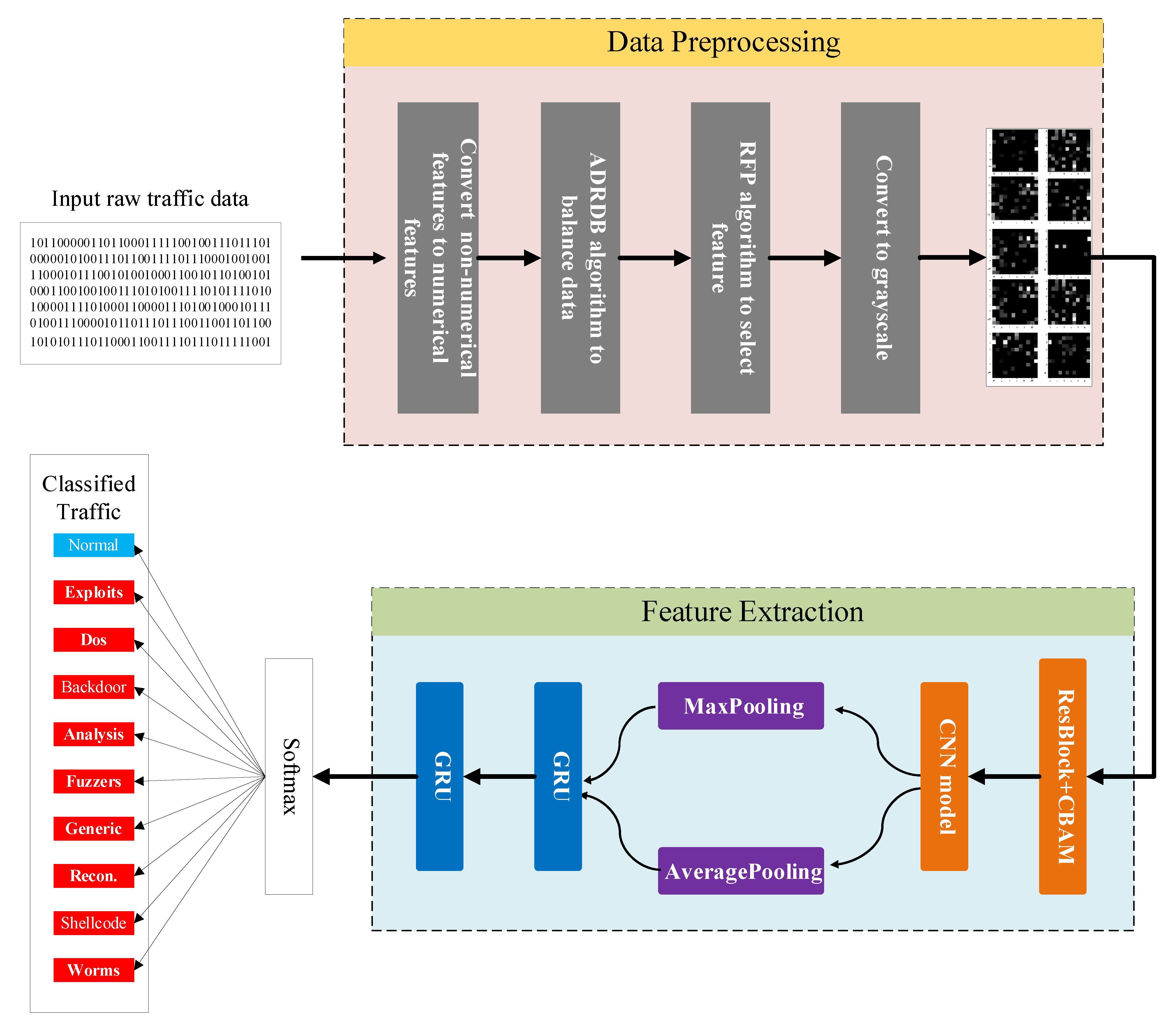
3. Network Intrusion Detection Model Based on CNN and GRU

Traditional intrusion detection models are more concerned with time series features and ignore spatial features in the process of detecting attacks. The CNN structure is more effective in extracting the spatial features of the data traffic, however, its ability to extract long-distance dependent information is mediocre; the GRU structure is more effective in extracting long-distance dependent information and can avoid forgetting during the learning process, however, its number of parameters is large and the training time is long. Therefore, this paper integrates the two to improve the model’s ability to learn features, which can fully extract features from both spatial and temporal dimensions, and thus achieve a higher classification detection accuracy.
The proposed network intrusion detection model combining convolutional neural network and GRU, referred to as the CNN-GRU model, consists of three main stages: firstly, the pre-processing stage, in which the original data is converted into numerical features and normalized, and then the dataset is balanced by the ADRDB algorithm, after which the features are extracted by the RFP algorithm and finally converted into a grey-scale map; Secondly, the training phase, in which the pre-processed data are assigned different weights to the features by the Convolutional Block Attention Module (CBAM) based on residuals firstly, then the spatial features are extracted by the CNN module, and the spatial information is further aggregated by combining Averagepooling and Maxpooling. After that, the temporal features are extracted by multiple GRU units. Finally, the classification is performed by the Softmax function; Thirdly, the testing phase, in which the test set is passed into the trained model for classification. The structure of the model proposed in this paper is shown in Figure 1.

3.1. Data Pre-Processing

In the pre-processing stage, this paper firstly converts the non-numerical features in the original flow data into numerical features and normalizes the features; secondly, a hybrid sampling algorithm (ADRDB algorithm) combining ADASYN and RENN is used for sampling; afterwards, the feature selection algorithm (RFP algorithm) is used for feature selection; finally, the resulting data is converted into a grey-scale map. The specific process of this stage is shown in Figure 1.

3.1.1. Non-Numerical Feature Transformation and Normalization

The only way the raw data can be used as model input is if it has been cleaned, labelled, annotated and prepared. In this paper, the LabelEncoder function in the scikit-learn library is used to convert the non-numeric features in the raw data traffic to numeric features to ensure that all feature values are numeric, thus facilitating the model to learn the data features.
When non-numeric features are converted to numeric, there is a tendency for the clustering of sample points in the feature space to be guided by individual feature values and less influenced by other feature values. Data normalization can reduce the variance of the features to a certain range, thus reducing the impact of outliers. In this paper, we use min–max normalization to normalize the feature values to between zero and one, as shown in the formula:
h i , j = h i , j min ( h i , j ) max ( h i , j ) min ( h i , j )
where h i , j represents the feature value in row i and column j of the dataset.
The normalized values are balanced by the proposed ADRDB algorithm for the majority and minority class samples, respectively, to obtain the balanced dataset. After that, the features are extracted by the RFP algorithm to obtain the pre-processed dataset.

3.1.2. Hybrid Sampling Method Combining ADASYN and RENN

The core idea of the hybrid sampling method proposed in this paper, which combines ADASYN and RENN, is as follows: firstly, divide the original data set into a majority class sample set and a minority class sample set; secondly, obtain a new majority class sample set by undersampling with the RENN algorithm for the majority class sample set, and obtain a new minority class sample set by oversampling with the ADASYN algorithm for the minority class sample set; thirdly, the DBSCAN clustering algorithm is used to remove the noise in the new sample set, and then the two datasets are merged to obtain the balanced dataset. The specific steps of the hybrid sampling method combining ADASYN and RENN are as follows. The detailed procedure is shown in Algorithm 1.
The inputs to the algorithm are the original majority class sample set N and minority class sample set P and the number of samples contained in both, and the outputs are the balanced majority class sample set newN and minority class sample set newP.
(1)
Calculate the degree of imbalance of the dataset d.
(2)
If d < d t h (where d t h is a pre-determined value for the maximum allowed degree of imbalance ratio), the following operations are performed: firstly, calculate the number of G samples that are needed to be generated for the minority class; secondly, for each sample in N find its k 1 nearest neighbors and calculate the ratio r i , where Δ i denotes the number of samples belonging to the majority class among the k nearest neighbors of and |X| all represent the number of samples; afterwards, normalize r i to r ^ i ; finally, calculate the number of samples that need to be synthesized for each minority class sample.
(3)
For each sample in N, generate g i samples in steps to obtain a new minority sample set.
(4)
For each sample in P, select k 2 nearest neighbor from newN.
(5)
Calculate the number of minority samples in the k 2 nearest neighbors of each majority sample and eliminate the sample if the number of samples is greater than e. (e = 1)
(6)
Repeat steps (4) and (5) to generate a new majority class sample set.
(7)
Remove the noise in newP and newN to get the final newN and newP.
Algorithm 1: Hybrid sampling method combining ADASYN and RENN (ADRDB)
Input:
  Minority class sample set, P.
  Majority class sample set, N.
Output:
  The balanced minority class sample set, newP.
  The balanced majority class sample set, newN.
Process:
(1) d = | P | / | N |
(2) If d < d t h
     G = ( | N | | P | ) × β
     for   each   i [ 1 , | P | ] do
         n e i g h b o r s P = g e t N e i g h b o r s ( P , N , k 1 )
         r i = Δ i / k 1
         r ^ i = r i / i = 1 m P r i
         g i = r ^ i × G
    end for
(3) x z i = c h o o s e ( x i , k 1 )
   for   each   i [ 1 , g i ] do
     x z i = c h o o s e ( x i , k 1 )
     s i = x i + ( x z i x i ) × λ
     P = [ P , s i ]
  end for
(4) n e w P = P
(5) C = | N | | n e w P |
(6) n e i g h b o r s N = g e t N e i g h b o r s ( N , n e w P , k 2 )
(7) for each j [ 1 , | N | ] do
     n u m N e g ( j ) = n e g N u m ( n e i g h b o r s N ( i ) )
     If   n u m P o s ( i ) > e
       N = r e m o v e ( i , N )
  end for
(8) Repeat (6), (7)
(9) n e w N = N
(10) DBSCAN Algorithm to remove noise
(11) Return   n e w P ,   n e w N

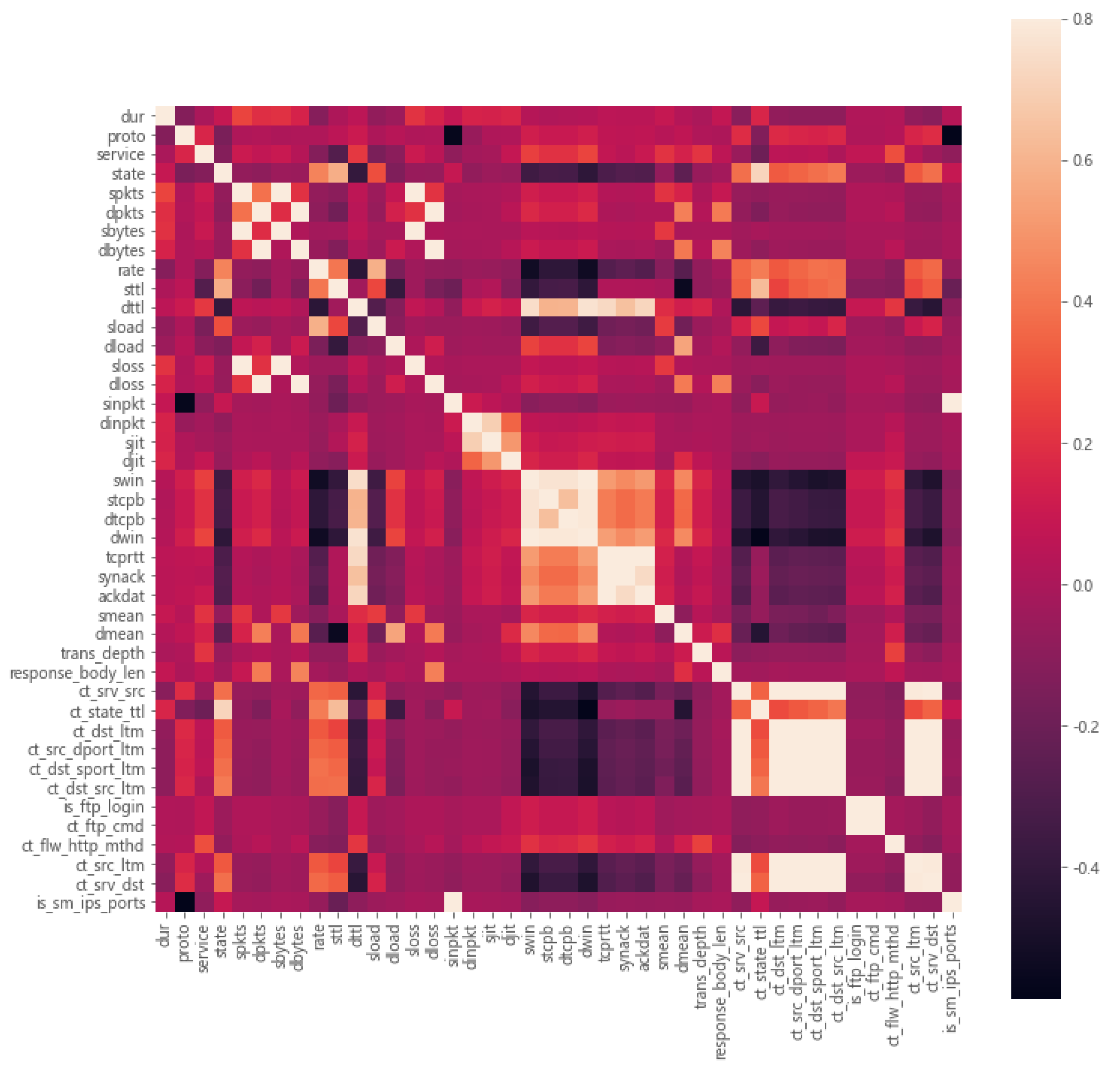
3.1.3. Feature Selection Algorithm

This paper proposes a new feature selection algorithm to address the problem of data features redundancy. The algorithm first calculates the importance of sample features by the Random Forest algorithm and ranks them in order of importance; then analyses the correlation between features by Pearson’s index; and finally combines the two results to select the features.
The Random Forest algorithm (RF) is an integrated learning algorithm using Decision Trees as the base learner. In feature engineering, RF algorithms can identify important features from a large number of sample features. The essence of the algorithm is to analyze and calculate the contribution of each feature of the sample in the tree, and then calculate its average value and compare the contribution between the features to identify the important features [46]. Existing methods are usually evaluated using the Gini index or the out-of-bag data error rate as an evaluation metric. The specific steps are as follows:
(1)
For each base learner, select the corresponding out-of-bag data (some of the remaining samples that are not selected) and calculate its error, denoted as error_a;
(2)
Randomly add disturbances to the full sample of out-of-bag data and calculate its error, noted as error_b;
(3)
Assuming that the forest contains M trees, the value of Importance of a feature is as follows:
I m p o r t a n c e = e r r o r _ b e r r o r _ a M
((4)
A new dataset is constructed by filtering out the features with a high level of importance.
The Pearson correlation coefficient is used to measure the correlation between two variables X and Y. It has a value range of (−1, 1) [47]. The Pearson correlation coefficient is obtained by calculating the covariance and standard deviation between the two eigenvalues and quoting it by the following formula:
ρ X , Y = cov ( X , Y ) σ X σ Y = E [ ( X μ X ) ( Y μ Y ) ] σ X σ Y
Pearson’s correlation coefficient varies from −1 to 1. If the Pearson’s correlation coefficient is close to ±1, this indicates a high correlation between the two characteristics and the relationship can be well represented by a linear equation. If the Pearson correlation coefficient is close to zero, it means that there is no linear relationship between the two features.
The pseudo code of the feature selection algorithm proposed in this paper is shown in Algorithm 2.
Algorithm 2: Feature selection algorithm (RFP)
Input:
  Original data set, D
Output:
  Processed dataset, NewD
Procedure:
(1)
Selecting out-of-bag data and calculating the error, noted as error_a.
(2)
Randomly add disturbances to the out-of-bag data, noted as error_b.
(3)
Calculating feature importance.
(4)
Ranking the importance of the features.
(5)
Calculating the Pearson correlation coefficient and performing a correlation analysis.
(6)
Combine steps (4) and (5) for feature selection.
(7)
Obtain the selected dataset, NewD.
The pre-processed dataset is obtained by converting the data after data balancing and feature selection into a grayscale map. The converted grayscale plots for the different categories are shown in Figure 2.

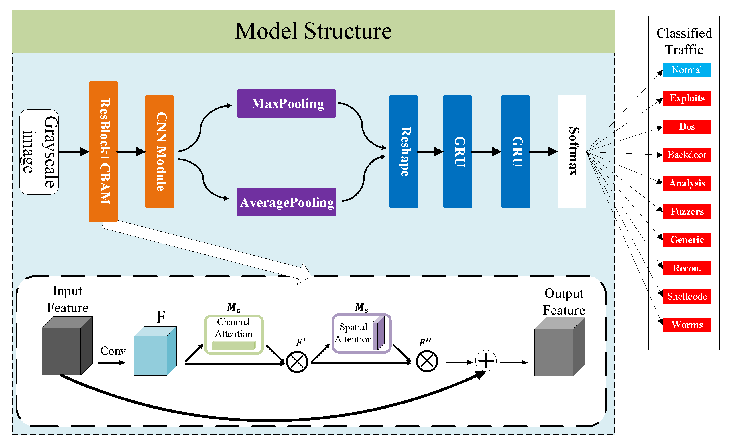
3.2. Model Structure

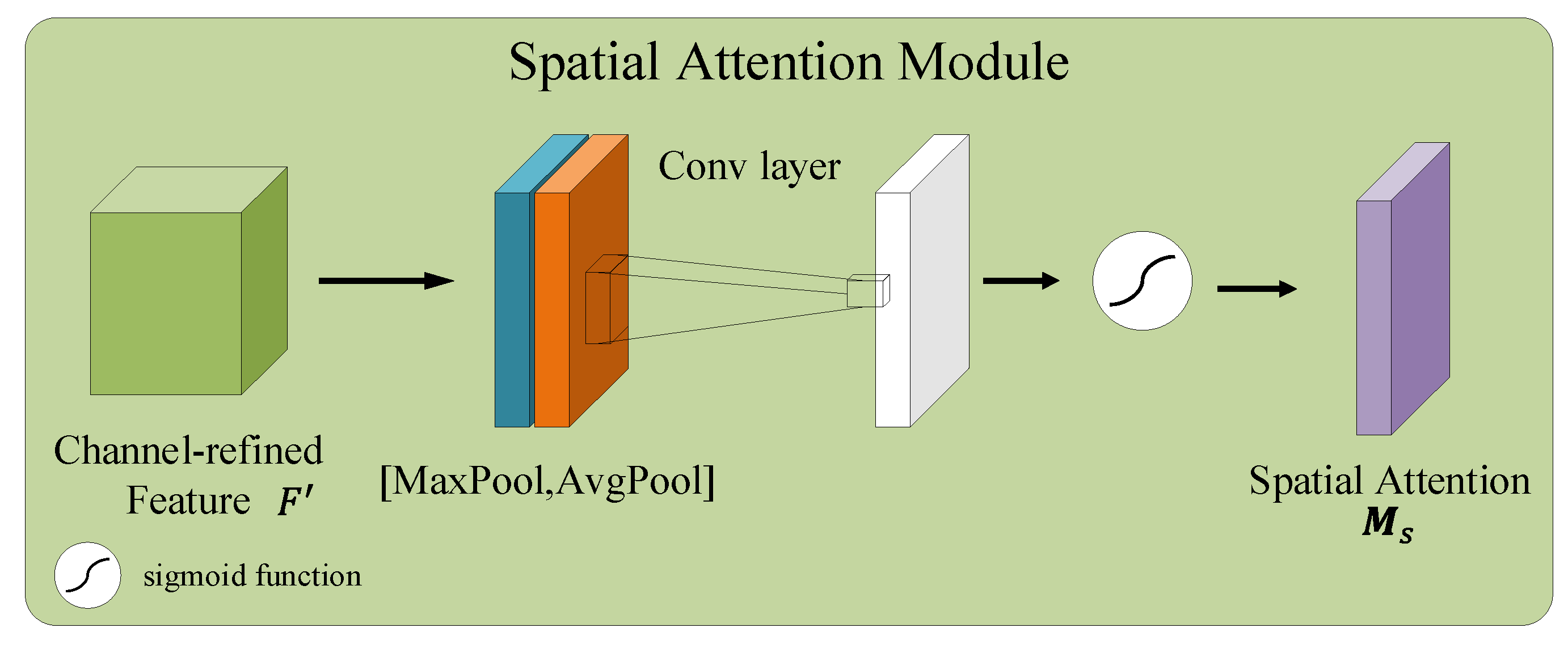
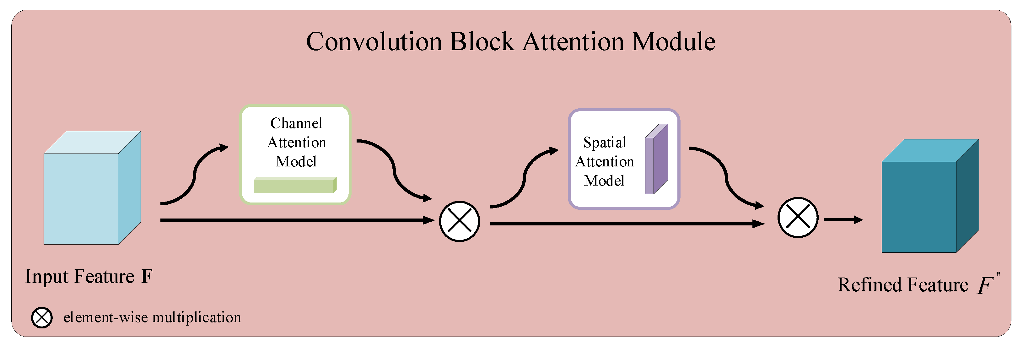
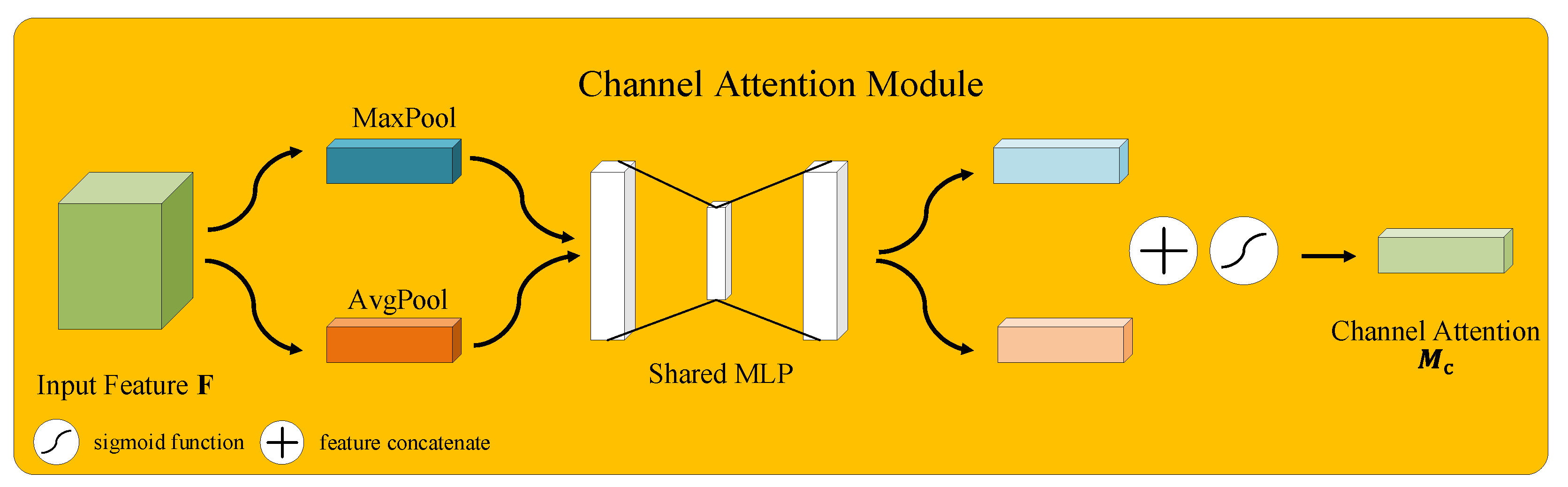
3.2.1. Convolutional Block Attention Module

The purpose of introducing an attention mechanism in the model is mainly to improve the representational power. It mainly means that we give a larger weight to important features and a smaller weight to unnecessary features. The Convolutional Block Attention Module (CBAM) is a lightweight attention module proposed by Woo et al. in 2018, which contains of two main parts: the channel attention module and the spatial attention module [48].
The specific structure of the channel attention module in CBAM is shown in Figure 3, which uses the relationship of features between channels to generate a channel attention map to form the input. Afterwards, the spatial information is aggregated using Averagepooling and Maxpooling, respectively, to generate two different sources of spatial information F a v g c and F max c . The two spatial information sources are fed into a shared network consisting of a multi-layer perceptron and a hidden layer, which in turn generate the required channel attention graph M c , and finally output the feature vector by element summation.
M c ( F ) = σ ( M L P ( A v g P o o l ( F ) ) + M L P ( M a x P o o l ( F ) ) ) = σ ( W 1 ( W 0 ( F a v g c ) ) + W 1 ( W 0 ( F max c ) ) )
where σ represents the sigmoid function, W 0 and W 1 are the weights of the multilayer perceptron, F is the input and M c is the final output.
The specific structure of the spatial attention module in CBAM is shown in Figure 4, which uses the spatial relationships between features to generate a spatial attention map to form the input. Afterwards, two 2D feature maps F a v g s and F max s are generated in turn by Averagepooling and Maxpooling, which effectively highlight the information region. The two are finally fused and the desired 2D spatial attention map is generated by standard convolution to output the feature vector.
M s ( F ) = σ ( f 7 × 7 ( [ A v g P o o l ( F ) ; M a x P o o l ( F ) ] ) ) = σ ( f 7 × 7 ( [ F a v g s ; F max s ] ) )
where f 7 × 7 represents a convolution operation with filter size 7 × 7 , F is the input and M s is the final output.
CBAM uses a channel attention module and a spatial attention module in turn, enabling the model to learn the features of the channel and spatial axes respectively, as shown in Figure 5. Given the initial feature map F as input, CBAM will generate 1D channel attention feature maps M c and 2D spatial attention feature maps M s in turn. The whole process is shown in Figure 5 and summarized as follows.
F = M c ( F ) F F = M s ( F ) F
where denotes element-wise multiplication, F is the output after the channel attention module and F is the final output.

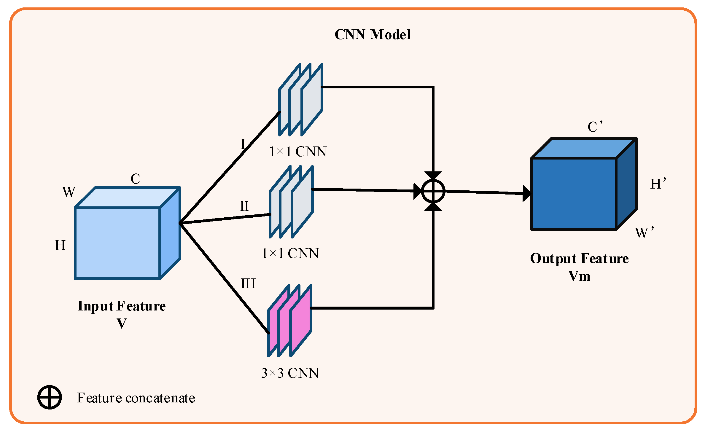
3.2.2. Convolutional Neural Networks

The two main existing and more popular CNN structures are the Residual Network (ResNet) [49] and the Inception Network [50], with ResNet proposing a concept of residual and Inception proposing a concept of split-transform-merge.
In order to improve the expressive power of CNN and to fully learn the diversity of features in the classification process, with the idea of Inception, the data input is extracted by multiple convolutional neural networks to ensure that they can learn simple to complex feature transformations. 2D convolution has shown excellent performance in the field of computer vision, so this paper uses 2D convolution to extract the spatial features of the data.
The CNN module used in this paper is described as follows: firstly, the processed grayscale maps are input to the strides as 1 × 1, 1 × 1 and 3 × 3 convolutional modules to extract features, respectively. After that, the resulting features are fused to obtain the processed feature maps. Its structure is shown in Figure 6.

3.2.3. Model Structure

The intrusion detection model proposed in this paper consists of three main parts: in order to comprehensively and finitely learn the features of the data, the features are firstly assigned different weights through the CBAM attention mechanism module based on residual; secondly, the spatial features are extracted through the CNN module, and the spatial information is further aggregated using fused Averagepooling and Maxpooling; then the temporal features are extracted through GRU, and finally the classification is carried out through the Softmax function, the specific structure of which is shown in Figure 7.
(1)
The grayscale map obtained after pre-processing is input to the CBAM module based on residual, and the features are given different weights to obtain the output F.
(2)
The new feature map F is input into the CNN module for feature extraction, after which the spatial information is aggregated using Maxpooling and Averagepooling to obtain the new feature map F C .
(3)
Pass F C to the GRU unit to extract the dependencies between features and obtain the output F G .
(4)
Pass F G to the fully connected layer, which uses Softmax as the activation function to achieve the classification of intrusion detection behavior.

4. Experimental Simulations

4.1. Experimental Setup

In order to test the performance of the proposed network intrusion detection method fusing CNN and GRU, several sets of experiments are designed in this paper.
  • Experiment 1: Feature selection analysis experiment
  • Experiment 2: Comparison of different feature selection methods
  • Experiment 3: Comparison of different sampling methods
  • Experiment 4: Comparison of single model and hybrid model
  • Experiment 5: Comparison of different pooling methods
  • Experiment 6: Performance comparison experiment
The intrusion detection model experiments and comparison experiments presented in this paper were conducted on a 64-bit Windows Intel(R) Core (TM) i7-7700HQ CPU (2.80 GHz) with 16 GB RAM and a python-based Nvidia GeForce GTX 1050 GPU (4 GB), using Python’s TensorFlow library to write the CNN and GRU models for this paper.
After several experimental validations, the parameters of the model in this paper are specified in Table 2.

4.2. Dataset and Evaluation Criteria

Over the years, many datasets related to intrusion detection have been introduced for research and development, including KDDCup99 [51], UNSW-NB15 [52], NSL-KDD [53], CIC-IDS2017 [54] and LITNET-2020 [55]. In this paper, we choose to use the UNSW-NB15, NSL-KDD and CIC-IDS2017 datasets to evaluate the proposed model. These datasets are the more widely used datasets in the existing intrusion detection field. The NSL-KDD dataset is a relatively early dataset applied to the field of intrusion detection, and the related research is more mature. UNSW_NB15 and CIC-IDS2017 are recent datasets that can better reflect the real network environment. The specific descriptions of the three datasets are shown below.
The NSL-KDD dataset is an improvement of the KDD99 dataset, which removes the redundant and duplicate data from the training and testing sets on the basis of the KDD99 dataset, so that the training and testing sets are set up in a more reasonable way. It mainly contains 41-dimensional attribute features and one-dimensional category features, covering five types of Normal, Probe, Dos, R2L, U2R. The distribution of different categories of attacks in the dataset is shown in Table 3.
The UNSW-NB15 dataset is a new dataset generated in 2015 by the Cyber Range Laboratory of the Australian Centre for Cyber Security (ACCS) using the IXIA PerfectStorm tool to simulate realistic cyber environments. The dataset mainly consists of 47 attribute features and two category features, and contains nine attack techniques: Fuzzers, Analysis, Backdoors, DoS, Exploits, Generic, Reconnaissance, Shellcode, Worms. In this paper, we directly use the initial training set and testing set to test the performance of the model. The distribution of different categories of attacks in the dataset is shown in Table 4.
The CIC-IDS2017 dataset is derived from the 3–7 July 2017 Canadian Institute for Cybersecurity (CIC) collection for cyber data, which contains benign as well as recent common attacks in the field of cyber intrusions, filling the gap of no cyber-based attacks in the UNSW-NB15 dataset. The dataset contains 78-dimensions of attribute features and one-dimension of category features covering 15 attack types. In this paper, the anomalous behaviors of a similar nature are merged, and the final dataset contains nine types of attacks: Benign, Dos, Portscan, Ddos, Patator, Bot, Web attack, Infiltration, and Heartbleed. The distribution of different categories of attacks in the dataset is shown in Table 5.
The evaluation metrics of the network security intrusion detection model include four main metrics: precision, accuracy, recall, and F1-score. In the specific detection results, T (true) and F (false) represent correctly or incorrectly classified data, respectively. P (positive) and N (negative) indicate that the predicted results of the detection system are abnormal or normal data, respectively. All data in the dataset must be classified into four categories: TP, TN, FP and FN. Only TP indicates that the system’s classification result consists of abnormal attack data and the classification result is correct; TN indicates that the system’s classification result is positive and correct; FP indicates that the system predicts the data as abnormal attack data although the classification result is wrong; FN indicates that the system predicts the data as normal data although the classification result is incorrect. The classification results of the model for the data are represented by the confusion matrix, as shown in Table 6.
Accuracy describes the ratio of the number of correct samples predicted to the total number of samples and is calculated as follows:
A ccuracy = T P + T N T P + F P + T N + F N
Precision describes the ratio of the number of classes predicted to be positive to the number of classes actually predicted to be positive, calculated as follows.
p r e c i s i o n = T P T P + F P
Recall describes the ratio of the number of predicted positive classes that are actually positive to the number of all positive classes and is calculated as follows.
r e c a l l = T P T P + F N
F 1 s c o r e describes the magnitude of the harmonic mean between precision and recall, calculated as follows.
F 1 s c o r e = 2 × r e c a l l × p r e c i s i o n r e c a l l + p r e c i s i o n
It can be seen that F 1 achieves larger values when both recall and precision have larger values.

4.3. Experimental Results and Analysis

In order to fully verify the effectiveness of the model proposed, several sets of experiments are set up in this paper: Section 4.3.1 sets up the feature selection analysis experiment to introduce the process and results of feature selection in detail; Section 4.3.2 sets up experiments on the comparison of different feature selection methods to compare the advantages and disadvantages of the RFP algorithm proposed in this paper, compared with existing algorithms used in the field of intrusion detection; Section 4.3.3 sets up experiments on the comparison of a single model and hybrid model to compare the advantages and disadvantages of the ADRDB algorithm proposed in this paper compared with other sampling methods; Section 4.3.4 sets up different sampling methods to verify the effectiveness of the proposed method; Section 4.3.5 sets up different pooling methods’ comparison experiments to analyze the effect of using only one pooling method and mixed pooling on the performance of the model; Section 4.3.6 sets up run-time comparison experiments to evaluate the run-time performance of the proposed model; Section 4.3.7 sets up performance analysis and comparison experiments to analyze the convergence of the CNN-GRU model, its effectiveness in detecting different classes, and also compares it with existing models. Section 4.3.8 sets up a statistical test to accurately evaluate the proposed intrusion detection method.

4.3.1. Experiment on Feature Selection Analysis

In order to verify the classification performance of the CNN-GRU algorithm proposed in this paper, the public dataset UNSW_NB15, NSL-KDD and CIC-IDS2017 were selected. This section focuses on the UNSW_NB15 dataset for detailed introduction. The detailed process of feature selection is mainly introduced for the RFP algorithm proposed in this paper.
In this paper, the importance of each feature in the dataset UNSW_NB15 is first calculated by the Random Forest algorithm and ranked according to the degree of importance, as shown in Figure 8. From the figure, it can be seen that the importance degree of different features varies greatly, for example, the importance value of feature sbytes is 0.115, while the importance value of is_ftp_login and ct_ftp_cmd is zero. The importance metrics of all features are distributed between 0 and 0.12.
Feature selection based on feature importance alone is a single reference criterion and the results obtained are not very convincing, so this paper combines feature importance and Pearson correlation analysis for feature selection. In order to visualize the correlation between features, a feature correlation diagram was created as shown in Figure 9. From the figure, the degree of correlation is clear between these 42-dimensional features. In order to further observe whether feature X and Y show correlation in the plane distribution, a correlation graph with feature X as the x-axis and feature Y as the y-axis is established. Due to the large number of data feature dimensions, this paper selects two types of features with correlation indices greater than or equal to 0.9 or less than or equal to −0.9 for analysis and introduction, as shown in Table 7.
Combining Figure 8 and Figure 9 for feature selection. For features with strong linear correlation, the more important features are retained according to the degree of importance; for features with weak linear correlation, the importance index of the features is analyzed, and if it is lower than 0.001, they are eliminated; for features whose correlation index is not within the analysis interval, their importance index is also analyzed, and those features with an importance level below 0.0001 are excluded. Finally, the NSL-KDD dataset leaves 28-dimensional features, the UNSW_NB15 dataset leaves 28-dimensional features, and the CIC-IDS2017 dataset leaves 52 features.

4.3.2. Comparison Experiments of Different Feature Selection Methods

In order to verify the effectiveness and applicability of the feature selection method proposed in this paper, a comparison experiment of different feature selection methods is set up in this section: the feature selection method (RFP) proposed in this paper is compared with existing feature selection methods such as PCA [23] and AE [24] under the same experimental conditions. The data obtained after pre-processing is first sampled using the ADRDB algorithm to balance the data set, and then the features of the NSL-KDD dataset are reduced to 28 dimensions; the features of the UNSW_NB15 dataset are reduced to 28 dimensions; and the features of the CIC-IDS2017 dataset are reduced to 52 dimensions by the above three methods, respectively. Finally, the classification experiments are conducted by the proposed model in the paper, and the model parameters are set as shown in Table 1. The results obtained are shown in Table 8. The bold text indicates the evaluation indicators of the proposed model.
From Table 8, it can be seen that the results obtained after using the data processed by the RFP algorithm proposed in this paper in the model are better. Analysis of the reasons for this shows that: the PCA method relies more on the variance when downscaling the data, while the non-principal components with small variance may also contain important information on the differences of the samples, and the downscaling process will have an impact on the subsequent data processing; the AE method is more dependent on the training data when reconstructing the feature space, thus, neither one of the above two methods has achieved better results. The RFP algorithm proposed in this paper starts from the data itself and selects features according to their importance and the correlation between them, which can improve the classification accuracy of the model.

4.3.3. Experiment Comparing Single Model with Hybrid Model

In order to verify the effectiveness of the model proposed in this paper on intrusion recognition, this section sets up performance analysis experiments on the intrusion detection model fusing CNN and GRU: under the same experimental conditions, the dataset was processed by sampling the preprocessing methods mentioned in Section 3.1 of the text, after which CNN, GRU and CNN-GRU were tested through the UNSW-NB15, NSL-KDD and CIC-IDS2017 datasets to obtain their classification accuracy, precision, recall and F1-score values as shown in Table 9. The bold text indicates the evaluation indicators of the proposed model.
As can be seen from the table, compared to using a single model of CNN and GRU, the CNN-GRU model can effectively extract the features of the original data and then effectively perform intrusion detection. The detection accuracy, recall, precision, and F1 score of dataset NSL-KDD reached 99.69%, 99.65%, 99.69%, and 99.70%, respectively; the detection accuracy, recall, precision, and F1 score of dataset UNSW_NB15 reached 86.25%, 86.92%, 86.25%, and 85.59%, respectively; and the detection accuracy, recall, precision, and F1 score of dataset CIC-IDS2017 reached 99.65%, 99.63%, 99.65%, and 99.64%, respectively. The reason for this is that the CNN structure can learn spatial features effectively by deepening the width of the network, while the GRU structure can extract temporal features of the data better. The model in this paper fuses CNN and GRU to learn both spatial and temporal features of the data, and introduces the attention mechanism to learn features comprehensively and effectively, thus achieving better results.

4.3.4. Comparison Experiments of Different Sampling Methods

In order to solve the problem of unbalanced dataset, this paper adopts a hybrid ADASYN and RENN sampling method (ADRDB algorithm) to process the dataset, in order to verify the effectiveness of the proposed method, this section sets up a comparison experiment of different sampling methods: under the same experimental conditions, the model uses seven different methods, SMOTE, ADASYN, random oversampler, ENN, RENN, random undersampler, and ADRDB, to handle the imbalanced data set. The RFP algorithm is then used to filter the features. Finally, the classification experiments are conducted by the proposed model in the paper, and the model parameters are set as shown in Table 1. The resulting detection accuracy is shown in Table 10. The bold text indicates the evaluation indicators of the proposed model.
As can be seen from the table, comparing a variety of different sampling methods, the ADRDB algorithm proposed in this paper has better processing effect for unbalanced samples. The reasons for the analysis are that the single oversampling methods such as Random Oversampler, SMOTE and ADASYN cannot effectively discriminate the noisy data and are prone to generate a large amount of noisy data in the process of synthesizing new samples, which in turn leads to the degradation of the classification effect of the model; the single undersampling methods such as Random Undersampler, ENN and RENN are prone to losing key information of most classes of samples, which in turn leads to the degradation of the classification effect of the model. In this paper, the proposed hybrid sampling method samples the majority and minority samples separately, and rejects the noisy data by the DBSCAN algorithm, which not only avoids the loss of key information, but also reduces the influence of noisy data on the classifier model, thus achieving better results.

4.3.5. Comparison Experiments with Different Pooling Methods

In this paper, we use a fusion of max pooling and average pooling to solve the problem of insufficient feature extraction ability of the model. To verify the effectiveness of the proposed method, this section sets up a comparison experiment of different pooling methods: under the same experimental conditions, the dataset is first processed by the preprocessing method mentioned in Section 3.1, and then the model is used to aggregate spatial information by three different methods: average pooling, maximum pooling, and fusion pooling, respectively. The model parameters are still used as those given in Table 1. The resulting detection accuracy is shown in Table 11. The bold text indicates the evaluation indicators of the proposed model.
The reason for this is that Averagepooling is used to extract features by averaging the global range of features, while Maxpooling is used to extract features by taking the maximum value of the feature points in the domain. The experimental results show that fusion pooling effectively improves the model’s ability to learn features, and the classification results are greatly improved.

4.3.6. Comparison Experiments of Run-Time Performance

To evaluate the run-time performance of the proposed model, this section sets up comparison experiments. Under the same experimental conditions, experiments are conducted for each of the following five scenarios to compare their training and prediction time and classification accuracy. These five scenarios are described as follows: (1) “Before RFP” means that the data is only sampled using the ADRDB algorithm during the data pre-processing stage, and then the data is converted into grayscale maps for input into the classification model; (2) “Before RFP” means that the data is not sampled using the ADRDB algorithm in the pre-processing stage, and the normalized data is only selected using the RFP algorithm, and then the data is converted into a grayscale map for input into the classification model; (3) “CNN” means that the data is preprocessed using the method described in Section 3.1, and then converted to grayscale maps for input into the classification model, which uses only the CNN structure; (4) “GRU” means that the data is preprocessed using the method described in Section 3.1, and then converted to grayscale maps for input into the classification model, which uses only the GRU structure; (5) “Proposed Model” indicates that the data are pre-processed using the method described in Section 3.1, and then the data are converted into grayscale maps for input into the proposed classification model. Besides, “Train” indicates the time taken to train the model for 200 epochs. The obtained experimental results are shown in Table 12. The bold text indicates the evaluation indicators of the proposed model.
From Table 12, the model proposed in this paper consumes more time than “CNN”, “GRU”,” Before ADRDB” and less time than “Before RFP”. The main reasons are as follows: The ADRDB algorithm generates new samples after the sampling is completed, resulting in more samples being used for training and testing, and thus takes more time. The RFP algorithm results in a decrease in the number of features in the samples after the feature selection is completed, and thus takes less time. When using a single CNN or GRU structure, the number of model parameters is smaller and thus the time spent is relatively less. The proposed model in this paper consumes relatively more time, however the model accuracy is greatly improved.

4.3.7. Performance Analysis and Comparison Experiments

Figure 10 gives a graph of the classification accuracy and loss value of the intrusion detection model CNN-GRU with the number of iteration steps. From the figure, it can be seen that the model in this paper achieves a good convergence effect.
In order to further verify the effectiveness of the intrusion detection model proposed in this paper, a performance comparison experiment is set up in this section: under the same experimental conditions, common machine learning methods such as random forest, K-mean clustering, decision tree and other recently proposed intrusion detection models are applied to the dataset, and the performance comparison is shown in Table 13. The bold text indicates the evaluation indicators of the proposed model.
Compared to machine learning algorithms, this model learns features through neural networks, which can combine low-level features to form a more abstract and non-linear high-level representation, and then explore the input–output relationship between data, effectively improving the accuracy of intrusion detection. Compared to the S-ResNet, CNN, CNN-GRU, CNN-LSTM, CNN-BiLSTM and CNN-GRU-attention models, the intrusion detection model CNN-GRU proposed in this paper reduces the effects of feature redundancy and class imbalance on the one hand, and can extract both spatial and temporal features of the data on the other hand, so that the extracted feature information is more comprehensive and thus achieves better results.

4.3.8. Statistical Test

In order to accurately evaluate the proposed intrusion detection method, significance tests were conducted on three datasets, UNSW_NB15, NSL-KDD, and CIC-IDS2017, with reference to the methods used in the literature [62,63]. We used a two-tailed t-test to analyze the significance of the indicators obtained by the proposed method and thus verify that the obtained results were not obtained by chance. The calculation formula is as follows:
μ = 1 n i = 1 n y ^ i
σ 2 = 1 n 1 i = 1 n ( y ^ i μ ) 2
t = n μ y 0 σ
We use the UNSW_NB15 dataset as an example for detailed discussion. First, the average accuracy value of the proposed method is calculated as 0.8625 according to Equation (10) (where y ^ i represents the i-th test accuracy value and n = 20). After that, the standard deviation of the accuracy value is calculated as 0.01040 by Equation (11). Finally, the critical value is X calculated by Equation (12) (where y 0 is the assumed minimum accuracy value and y 0 = 0.8438). The critical value 5.268 is greater than the 2.845 obtained in the two-tailed t-test table. This result indicates that the tested accuracy value of our proposed model is greater than the assumed minimum value of 0.8438, which has a confidence degree of ( 1 α = 0.99 ). The experimental results for the three data sets are shown in Table 14.
From Table 14, the minimum values of our assumed accuracies are all higher than the maximum values of the different models mentioned in the paper. Therefore, the model proposed in the paper has a statistically significant difference compared to the single use of the CNN model, GRU model and other existing models, and has a significant advantage over other methods.

5. Conclusions

Traditional intrusion detection models generally suffer from incomplete feature extraction and general multi-classification effects. To address these problems, this paper proposes an intrusion detection model that fuses convolutional neural networks and gated recursive units. The model solves the problems of data set imbalance and feature redundancy by using the ADRDB algorithm and the RFP algorithm, and then achieves comprehensive and sufficient feature learning by fusing CNN and GRU, while introducing the attention module to assign different weights to the features, thus reducing the overhead and improving the model performance. The accuracy of the proposed model based on the NSL-KDD dataset, UNSW_NB15 dataset and CIC-IDS2017 dataset is 99.69%, 86.25% and 99.65%, respectively. Furthermore, the precision can reach 99.65%, 86.92% and 99.63%.
In summary, This paper demonstrates that the model has a strong feature extraction capability, high detection accuracy and low false alarm rate when dealing with large-scale high-dimensional network data through feature selection analysis experiments, hybrid model versus single model comparison experiments, feature extraction method comparison experiments, pooling method comparison experiments and performance analysis experiments on the dataset, and has greatly improved the detection effect for a few classes, which provides promising prospective real-time applications for intrusion detection systems.
However, the model proposed in this paper still has some drawbacks while improving the detection accuracy: first, the number of parameters of the model is relatively high; second, the running time of the model is relatively high; third, the detection accuracy of the model for a small number of samples is improved, although the improvement effect is not much. In the subsequent research, we will further study the model lightweighting to further improve the accuracy of minority sample detection, further improve the overall classification effect of the model, and further reduce the running time cost.

Author Contributions

Resources, Y.S. and Y.Q.; Visualization, C.C.; Validation, B.C.; Writing—review and editing, B.C.; Supervision, C.L. All authors have read and agreed to the published version of the manuscript.

Funding

This work is supported by the National Science Foundation of China (61806219, 61703426 and 61876189), by Young Talent fund of University and Association for Science and Technology in Shaanxi, China (20190108), and by and the Innovation Capability Support Plan of Shaanxi, China (2020KJXX-065).

Data Availability Statement

All data used in this paper can be obtained by contacting the authors of this study.

Conflicts of Interest

The authors declare no conflict of interest.

References

  1. Yang, L.; Quan, Y. Dynamic Enabling Cyberspace Defense; People’s Posts and Telecommunications Press: Beijing, China, 2018. [Google Scholar]
  2. Yu, N. A Novel Selection Method of Network Intrusion Optimal Route Detection Based on Naive Bayesian. Int. J. Appl. Decis. Sci. 2018, 11, 1–17. [Google Scholar] [CrossRef]
  3. Ren, X.K.; Jiao, W.B.; Zhou, D. Intrusion Detection Model of Weighted Navie Bayes Based on Particle Swarm Optimization Algorithm. Comput. Eng. Appl. 2016, 52, 122–126. [Google Scholar]
  4. Koc, L.; Mazzuchi, T.A.; Sarkani, S. A network intrusion detection system based on a Hidden Naïve Bayes multiclass classifier. Expert Syst. Appl. 2012, 39, 13492–13500. [Google Scholar] [CrossRef]
  5. Teng, L.; Teng, S.; Tang, F.; Zhu, H.; Zhang, W.; Liu, D.; Liang, L. A Collaborative and Adaptive Intrusion Detection Based on SVMs and Decision Trees. In Proceedings of the IEEE International Conference on Data Mining Workshop, Shenzhen, China, 14 December 2014; pp. 898–905. [Google Scholar] [CrossRef]
  6. Chen, S.X.; Peng, M.L.; Xiong, H.L.; Yu, X. SVM Intrusion Detection Model Based on Compressed Sampling. J. Electr. Comput. Eng. 2016, 2016, 6. [Google Scholar] [CrossRef] [Green Version]
  7. Reddy, R.R.; Ramadevi, Y.; Sunitha, K.V.N. Effective discriminant function for intrusion detection using SVM. In Proceedings of the International Conference on Advances in Computing, Communications and Informatics (ICACCI), Jaipur, India, 21–24 September 2016; pp. 1148–1153. [Google Scholar]
  8. Tao, Z.; Sun, Z. An Improved Intrusion Detection Algorithm Based on GA and SVM. IEEE Access 2018, 6, 13624–13631. [Google Scholar] [CrossRef]
  9. Wang, H.W.; Gu, J.; Wang, S.S. An Effective Intrusion Detection Framework Based on SVM with Feature Augmentation. Knowl.-Based Syst. 2017, 136, 130–139. [Google Scholar] [CrossRef]
  10. Sahu, S.K.; Katiyar, A.; Kumari, K.M.; Kumar, G.; Mohapatra, D.P. An SVM-Based Ensemble Approach for Intrusion Detection. Int. J. Inf. Technol. Web Eng. 2019, 14, 66–84. [Google Scholar] [CrossRef]
  11. Sahu, S.; Mehtre, B.M. Network intrusion detection system using J48 Decision Tree. In Proceedings of the International Conference on Advances in Computing, Communications and Informatics (ICACCI), Kochi, India, 10–13 August 2015; pp. 2023–2026. [Google Scholar] [CrossRef]
  12. Jiang, F.; Chun, C.P.; Zeng, H.F. Relative Decision Entropy Based Decision Tree Algorithm and Its Application in Intrusion Detection. Comput. Sci. 2012, 39, 223–226. [Google Scholar]
  13. Ahmim, A.; Maglaras, L.A.; Ferrag, M.A.; Derdour, M.; Janicke, H. A Novel Hierarchical Intrusion Detection System Based on Decision Tree and Rules-Based Models. In Proceedings of the 15th International Conference on Distributed Computing in Sensor Systems (DCOSS), Santorini Island, Greece, 29–31 May 2019; pp. 228–233. [Google Scholar] [CrossRef] [Green Version]
  14. Yun, W. A Multinomial Logistic Regression Modeling Approach for Anomaly Intrusion Detection. Comput. Secur. 2005, 24, 662–674. [Google Scholar] [CrossRef]
  15. Kamarudin, M.H.; Maple, C.; Watson, T.; Sofian, H. Packet Header Intrusion Detection with Binary Logistic Regression Approach in Detecting R2L and U2R Attacks. In Proceedings of the Fourth International Conference on Cyber Security, Cyber Warfare, and Digital Forensic (CyberSec), Jakarta, Indonesia, 29–31 October 2015; pp. 101–106. [Google Scholar] [CrossRef] [Green Version]
  16. Ioannou, C.; Vassiliou, V. An Intrusion Detection System for Constrained WSN and IoT Nodes Based on Binary Logistic Regression. In Proceedings of the 21st ACM International Conference on Modeling, Analysis and Simulation of Wireless and Mobile Systems, Montreal, QC, Canada, 28 October–2 November 2018; pp. 259–263. [Google Scholar] [CrossRef]
  17. LeCun, Y.; Bengio, Y.; Hinton, G. Deep Learning. Nature 2015, 521, 436–444. [Google Scholar] [CrossRef]
  18. Krizhevsky, A.; Sutskever, I.; Hinton, G.E. ImageNet Classification with Deep Convolutional Neural Networks. In Proceedings of the Annual Conference on Neural Information Processing Systems (NIPS), Lake Tahoe, NV, USA, 3–6 December 2012; pp. 1106–1114. [Google Scholar]
  19. Yuqing, Z.; Ying, D.; Caiyun, L.; Kenan, L.; Hongyu, S. Situation, trends and prospects of deep learning applied to cyberspace security. J. Comput. Res. Dev. 2018, 55, 1117–1142. [Google Scholar]
  20. Javaid, A.; Niyaz, Q.; Sun, W.; Alam, M. A deep learning approach for network intrusion detection system. In Proceedings of the 9th EAI International Conference on Bio-inspired Information and Communications Technologies, New York, NY, USA, 3–5 December 2015; ACM Press: New York, NY, USA, 2016; pp. 21–26. [Google Scholar]
  21. Wei, W.; Sheng, Y.; Wang, J.; Zeng, X.; Ye, X.; Huang, Y.; Zhu, M. HAST-IDS: Learning Hierarchical Spatial-Temporal Features Using Deep Neural Networks to Improve Intrusion Detection. IEEE Access 2018, 6, 1792–1806. [Google Scholar] [CrossRef]
  22. Zexuan, M.; Jin, L.; Yanli, L.; Chen, C. A network intrusion detection method incorporating WaveNet and BiGRU. Syst. Eng. Electron. Technol. 2021, 11, 1–12. [Google Scholar]
  23. Liu, J.; Sun, X.; Jin, J. Intrusion detection model based on principal component analysis and cyclic neural network. Chin. J. Inf. Technol. 2020, 34, 105–112. [Google Scholar]
  24. Zhou, P.; Zhou, Z.; Wang, L.; Zhao, W. Network intrusion detection method based on autoencoder and RESNET. Comput. Appl. Res. 2020, 37, 224–226. [Google Scholar]
  25. Yan, B.H.; Han, G.D. Combinatorial Intrusion Detection Model Based on Deep Recurrent Neural Network and Improved SMOTE Algorithm. Chin. J. Netw. Inf. Secur. 2018, 4, 48–59. [Google Scholar]
  26. He, H.; Bai, Y.; Garcia, E.A.; Li, S. ADASYN: Adaptive synthetic sampling approach for imbalanced learning. In Proceedings of the IEEE International Joint Conference on Neural Networks (IEEE World Congress on Computational Intelligence), Hong Kong, China, 1–8 June 2008; pp. 1322–1328. [Google Scholar] [CrossRef] [Green Version]
  27. Wang, L.; Han, M.; Li, X.; Zhang, N.; Cheng, H. Review of Classification Methods on Unbalanced Data Sets. IEEE Access 2021, 9, 64606–64628. [Google Scholar] [CrossRef]
  28. Deng, Y.W.; Pu, H.T.; Hua, X.B.; Sun, B. Research on lane line detection based on RC-DBSCAN. J. Hunan Univ. 2021, 48, 85–92. [Google Scholar]
  29. Tama, B.A.; Comuzzi, M.; Rhee, K.H. TSE-IDS: A two-stage classifier ensemble for intelligent anomaly-based intrusion detection system. IEEE Access 2019, 7, 94497–94507. [Google Scholar] [CrossRef]
  30. Bu, S.J.; Cho, S.B. A convolutional neural-based learning classifier system for detecting database intrusion via insider attack. Inf. Sci. 2020, 512, 123–136. [Google Scholar] [CrossRef]
  31. Le, T.-T.-H.; Kim, Y.; Kim, H. Network Intrusion Detection Based on Novel Feature Selection Model and Various Recurrent Neural Networks. Appl. Sci. 2019, 9, 1392. [Google Scholar] [CrossRef] [Green Version]
  32. Hassan, M.M.; Gumaei, A.; Alsanad, A.; Alrubaian, M.; Fortino, G. A hybrid deep learning model for efficient intrusion detection in big data environment. Inf. Sci. 2020, 513, 386–396. [Google Scholar] [CrossRef]
  33. Louk, M.H.L.; Tama, B.A. Exploring Ensemble-Based Class Imbalance Learners for Intrusion Detection in Industrial Control Networks. Big Data Cogn. Comput. 2021, 5, 72. [Google Scholar] [CrossRef]
  34. Liu, L.; Wang, P.; Lin, J.; Liu, L. Intrusion detection of imbalanced network traffic based on machine learning and deep learning. IEEE Access 2021, 9, 7550–7563. [Google Scholar] [CrossRef]
  35. Yan, M.; Chen, Y.; Hu, X.; Cheng, D.; Chen, Y.; Du, J. Intrusion detection based on improved density peak clustering for imbalanced data on sensor-cloud systems. J. Syst. Archit. 2021, 118, 102212. [Google Scholar] [CrossRef]
  36. Alharbi, A.; Alosaimi, W.; Alyami, H.; Rauf, H.T.; Damaševičius, R. Botnet Attack Detection Using Local Global Best Bat Algorithm for Industrial Internet of Things. Electronics 2021, 10, 1341. [Google Scholar] [CrossRef]
  37. Toldinas, J.; Venčkauskas, A.; Damaševičius, R.; Grigaliūnas, Š.; Morkevičius, N.; Baranauskas, E. A Novel Approach for Network Intrusion Detection Using Multistage Deep Learning Image Recognition. Electronics 2021, 10, 1854. [Google Scholar] [CrossRef]
  38. Khan, M.A. HCRNNIDS: Hybrid Convolutional Recurrent Neural Network-Based Network Intrusion Detection System. Processes 2021, 9, 834. [Google Scholar] [CrossRef]
  39. Pu, G.; Wang, L.; Shen, J.; Dong, F. A hybrid unsupervised clustering-based anomaly detection method. Tsinghua Sci. Technol. 2021, 26, 146–153. [Google Scholar] [CrossRef]
  40. Nguyen, G.N.; Viet, N.H.L.; Elhoseny, M.; Shankar, K.; Gupta, B.B.; Abd El-Latif, A.A. Secure blockchain enabled Cyber-physical systems in healthcare using deep belief network with ResNet model. J. Parallel Distrib. Comput. 2021, 153, 150–160. [Google Scholar] [CrossRef]
  41. Panigrahi, R.; Borah, S.; Bhoi, A.K.; Ijaz, M.F.; Pramanik, M.; Kumar, Y.; Jhaveri, R.H. A Consolidated Decision Tree-Based Intrusion Detection System for Binary and Multiclass Imbalanced Datasets. Mathematics 2021, 9, 751. [Google Scholar] [CrossRef]
  42. Injadat, M.; Moubayed, A.; Nassif, A.B.; Shami, A. Multi-Stage Optimized Machine Learning Framework for Network Intrusion Detection. IEEE Trans. Netw. Serv. Manag. 2021, 18, 1803–1816. [Google Scholar] [CrossRef]
  43. Lv, Z.; Chen, D.; Lou, R.; Song, H. Industrial Security Solution for Virtual Reality. IEEE Internet Things J. 2021, 8, 6273–6281. [Google Scholar] [CrossRef]
  44. Zhou, X.; Liang, W.; Shimizu, S.; Ma, J.; Jin, Q. Siamese Neural Network Based Few-Shot Learning for Anomaly Detection in Industrial Cyber-Physical Systems. IEEE Trans. Ind. Inform. 2021, 17, 5790–5798. [Google Scholar] [CrossRef]
  45. Zhou, X.; Hu, Y.; Liang, W.; Ma, J.; Jin, Q. Variational LSTM Enhanced Anomaly Detection for Industrial Big Data. IEEE Trans. Ind. Inform. 2021, 17, 3469–3477. [Google Scholar] [CrossRef]
  46. Gregorutti, B.; Michel, B.; Saint-Pierre, P. Correlation and variable importance in random forests. Stat. Comput. 2017, 27, 659–678. [Google Scholar] [CrossRef] [Green Version]
  47. LeCun, Y.; Bottou, L.; Bengio, Y.; Haffner, P. Gradient-based learning applied to document recognition. Proc. IEEE 1998, 86, 2278–2324. [Google Scholar] [CrossRef] [Green Version]
  48. Woo, S.; Park, J.; Lee, J.Y.; Kweon, I.S. CBAM: Convolutional Block Attention Module. In Computer Vision—ECCV 2018. ECCV 2018. Lecture Notes in Computer Science; Ferrari, V., Hebert, M., Sminchisescu, C., Weiss, Y., Eds.; Springer: Cham, Switzerland, 2018; Volume 11211. [Google Scholar] [CrossRef] [Green Version]
  49. He, K.; Zhang, X.; Ren, S.; Sun, J. Deep Residual Learning for Image Recognition. In Proceedings of the 2016 IEEE Conference on Computer Vision and Pattern Recognition (CVPR), Las Vegas, NV, USA, 27–30 June 2016; pp. 770–778. [Google Scholar] [CrossRef] [Green Version]
  50. Xie, S.; Girshick, R.; Dollár, P.; Tu, Z.; He, K. Aggregated residual transformations for deep neural networks. In Proceedings of the 2017 IEEE Conference on Computer Vision and Pattern Recognition (CVPR), Honolulu, HI, USA, 21–26 July 2017; pp. 5987–5995. [Google Scholar] [CrossRef] [Green Version]
  51. Lippmann, R.; Haines, J.W.; Fried, D.J.; Korba, J.; Das, K. Analysis and Results of the 1999 DARPA Off-Line Intrusion Detection Evaluation. In Recent Advances in Intrusion Detection. RAID 2000; Lecture Notes in Computer Science; Debar, H., Mé, L., Wu, S.F., Eds.; Springer: Berlin/Heidelberg, Germany, 2000; Volume 1907. [Google Scholar] [CrossRef] [Green Version]
  52. Zhang, H.; Li, J.L.; Liu, X.M.; Dong, C. Multi-dimensional feature fusion and stacking ensemble mechanism for network intrusion detection. Future Gener. Comput. Syst. 2021, 122, 130–143. [Google Scholar] [CrossRef]
  53. Tavallaee, M.; Bagheri, E.; Lu, W.; Ghorbani, A.A. A detailed analysis of the KDD CUP 99 data set. In Proceedings of the 2009 IEEE Symposium on Computational Intelligence for Security and Defense Applications, Ottawa, ON, Canada, 8–10 July 2009; pp. 1–6. [Google Scholar] [CrossRef] [Green Version]
  54. Rosay, A.; Riou, K.; Carlier, F.; Leroux, P. Multi-layer perceptron for network intrusion detection. Ann. Telecommun. 2021, 6, 1–24. [Google Scholar] [CrossRef]
  55. Damasevicius, R.; Venckauskas, A.; Grigaliunas, S.; Toldinas, J.; Morkevicius, N.; Aleliunas, T.; Smuikys, P. LITNET-2020: An Annotated Real-World Network Flow Dataset for Network Intrusion Detection. Electronics 2020, 9, 800. [Google Scholar] [CrossRef]
  56. Xiao, Y.; Xiao, X. An Intrusion Detection System Based on a Simplified Residual Network. Information 2019, 10, 356. [Google Scholar] [CrossRef] [Green Version]
  57. Xiao, Y.; Xing, C.; Zhang, T.; Zhao, Z. An Intrusion Detection Model Based on Feature Reduction and Convolutional Neural Networks. IEEE Access 2019, 7, 42210–42219. [Google Scholar] [CrossRef]
  58. Xie, X.; Wang, B.; Wan, T.; Tang, W. Multivariate Abnormal Detection for Industrial Control Systems Using 1D CNN and GRU. IEEE Access 2020, 8, 88348–88359. [Google Scholar] [CrossRef]
  59. Sinha, J.; Manollas, M. Efficient deep CNN-BILSTM model for network intrusion detection. In Proceedings of the 3rd International Conference on Artificial Intelligence and Pattern Recognition, Xiamen, China, 26–28 June 2020; pp. 223–231. [Google Scholar] [CrossRef]
  60. Niu, Q.; Li, X. A High-performance Web Attack Detection Method based on CNN-GRU Model. In Proceedings of the IEEE 4th Information Technology, Networking, Electronic and Automation Control Conference (ITNEC), Chongqing, China, 12–14 June 2020; pp. 804–808. [Google Scholar] [CrossRef]
  61. Jiang, Y.; Jia, M.; Zhang, B.; Deng, L. Malicious Domain Name Detection Model Based on CNN-GRU-Attention. In Proceedings of the 33rd Chinese Control and Decision Conference (CCDC), Kunming, China, 22–24 May 2021; pp. 1602–1607. [Google Scholar] [CrossRef]
  62. Hu, J.; Zheng, W. A deep learning model to effectively capture mutation information in multivariate time series prediction. Knowl.-Based Syst. 2020, 203, 106139. [Google Scholar] [CrossRef]
  63. Teng, F.; Guo, X.; Song, Y.; Wang, G. An Air Target Tactical Intention Recognition Model Based on Bidirectional GRU With Attention Mechanism. IEEE Access 2021, 9, 169122–169134. [Google Scholar] [CrossRef]
Figure 1. Network Intrusion Detection Model Based on CNN and GRU.
Applsci 12 04184 g001
Figure 2. Converted grayscale map.
Applsci 12 04184 g002
Figure 3. Channel Attention Module.
Applsci 12 04184 g003
Figure 4. Spatial attention module.
Applsci 12 04184 g004
Figure 5. Convolutional block attention module.
Applsci 12 04184 g005
Figure 6. CNN structure.
Applsci 12 04184 g006
Figure 7. Intrusion detection model structure diagram. denotes element-wise multiplication and denotes feature concatenate.
Applsci 12 04184 g007
Figure 8. Feature importance map for the UNSW_NB15 dataset.
Applsci 12 04184 g008
Figure 9. Heat map of features in the UNSW_NB15 dataset.
Applsci 12 04184 g009
Figure 10. Accuracy and loss value curves with iteration steps: (a) Accuracy, loss value with the number of iteration steps curve of the NSL-KDD dataset; (b) Accuracy, loss value with the number of iteration steps curve of the UNSW_NB15 dataset; (c) Accuracy, loss value with the number of iteration steps curve of the CIC-IDS2017 dataset.
Applsci 12 04184 g010
Table 1. A brief description of the recent related works on network intrusion detection, using several optimization, deep, and machine learning algorithms.
Ref.DatasetMethodsEvaluation MetricsAccuracy
[36]N-BaIoTLGBA-NNprecision, recall
F1-score, support
Gained 90% accuracy
[37]UNSW_NB15
BOUN Ddos
ML.NETprecision, ROC
confusion matrix
99.8% of the generic attack
99.7% of the Ddos attack
[38]CSE-CIC-IDS2018HRCNNIDSprecision, recall
F1-score, DR, FAR
Gained 97.75% accuracy
[39]NSL-KDDSSC-OCSVMrecall, FAR, ROC
confusion matrix
Obtained satisfactory results
[40]NSL-KDD 2015
CIDDS-001
Proposed DBNprecision, recall
F1-score, accuracy
Obtained satisfactory results
[41]NSL-KDD
CICIDS2017
SRRS + IIFS-MC(ALL) + CTCDR, FPR, accuracy99.96% of NSL-KDD
99.95% of CICIDS2017
[42]CICIDS2017
UNSW-NB15
NIDS-sprecision, recall
FAR, accuracy
Gained 99% accuracy of two datasets
[43]KDDCUP1999CSWC-SVMprecision, accuracyObtained satisfactory results
[44]UNSW_NB15FSL-SCNNprecision, recall
F1-score, FAR
Obtained satisfactory results
[45]UNSW_NB15VLSTMprecision, recall
F1-score, FAR, AUC
Gained 86% accuracy
Table 2. Model parameter settings.
Model ParametersParameter Settings
Batch size1024
Loss functionSparseCategoricalCrossentropy
OptimizerSGD
Optimizer learning rate0.001
Epoch200
Resblock + CBAM64
GRU32/64/128
Dropout0.5
Table 3. Distribution of different attack behaviors in the NSL-KDD dataset.
DatasetAttack BehaviorTotal
NormalDosProbeR2LU2R
KDDTrain+67,34345,92711,65699552125,973
KDDTest+98897460270724216722,544
Total77,23253,38714,3633416119148,517
Table 4. Distribution of different attack behaviors in the UNSW_NB15 dataset.
DatasetAttack BehaviorsTotal
NormalFuzzersAnalysisBackdoorsDoSExploitsGenericRecon.ShellcodeWorms
Train56,00018,1742000174612,26433,39340,00010,4911133130175,341
Test37,0006062677583408911,13218,87134963784482,332
Total93,00024,2462677232916,35344,52558,87113,9871511174257,673
Table 5. Distribution of different attack behaviors in the CIC-IDS2017 dataset.
DatasetAttack BehaviorsTotal
BENIGNDosPortScanPatatorDdosBotWeb AttackInfiltrationHeartbleed
Train1,654,737176,863111,251968589,619275215262572,046,465
Test709,17375,79847,679415038,4081180654114877,057
Total2,363,910252,661158,93013,835128,0273932218036112,923,522
Table 6. Confusion matrix.
ClassificationPredicted Positive CategoryPredicted Negative Category
Actual Positive CategoryTPFN
Actual Negative CategoryFPTN
Table 7. Feature Correlation Index.
FeaturesCorrelation IndexFeaturesCorrelation Index
spktssbytes0.964tcprttsynack0.943
spktssloss0.972tcprttackdat0.920
dpktsdbytes0.973ct_srv_srcct_dst_src_ltm0.954
dpktsdloss0.980ct_srv_srcct_srv_dst0.949
sbytessloss0.996ct_dst_ltmct_src_dport_ltm0.962
dbytesdloss0.997ct_dst_ltmct_src_ltm0.902
sinpktis_sm_ips_ports0.942ct_src_dport_ltmct_dst_sport_ltm0.908
swindwin0.980ct_src_dport_ltmct_src_ltm0.909
ct_dst_src_ltmct_srv_dst0.960is_ftp_loginct_ftp_cmd0.999
Table 8. Comparison of different feature selection methods.
DatasetFeature Selection MethodEvaluation Indicators (%)
AccuracyPrecisionRecallF1-Score
NSL-KDDRFP99.6999.6599.6999.70
PCA98.2698.7998.2698.48
AE97.6197.6397.6197.59
UNSW_NB15RFP86.2586.9286.2586.59
PCA79.3779.7079.3776.92
AE81.0180.4381.0180.05
CIC-IDS2017RFP99.6599.6399.6599.64
PCA89.6493.0289.6490.60
AE98.6698.7098.6698.67
Table 9. Comparison of single and hybrid models.
DatasetFeature Selection MethodEvaluation Indicators (%)
AccuracyPrecisionRecallF1-Score
NSL-KDDCNN98.2298.2398.2298.18
GRU98.6798.9598.6798.78
CNN-GRU99.6999.6599.6999.70
UNSW_NB15CNN84.5184.0884.5184.29
GRU83.6983.8183.6883.74
CNN-GRU86.2586.9286.2586.59
CIC-IDS2017CNN92.9493.2492.9492.04
GRU98.1598.3698.1598.16
CNN-GRU99.6599.6399.6599.64
Table 10. Comparison of different sampling methods.
DatasetFeature Selection MethodEvaluation Indicators (%)
AccuracyPrecisionRecallF1-Score
NSL-KDDRandom Oversampler92.7995.1292.7993.74
Random Undersampler84.8393.2684.9387.04
SMOTE98.9799.0398.9798.99
ADASYN98.3598.8398.3598.57
ENN98.8598.8798.8598.85
RENN98.0298.0698.0298.03
ADASYN + RENN99.6999.6599.6999.70
UNSW_NB15Random Oversampler81.9082.2781.9079.33
Random Undersampler73.0979.6973.0972.33
SMOTE83.5181.0883.5182.71
ADASYN83.0480.6983.0484.23
ENN80.1278.9880.1277.49
RENN81.4081.9381.4081.66
ADASYN + RENN86.2586.9286.2586.59
CIC-IDS2017Random Oversampler96.0995.8796.0995.98
Random Undersampler17.2481.4817.2417.46
SMOTE92.1392.1392.1392.03
ADASYN97.3897.4197.3897.36
ENN95.2095.5195.2094.74
RENN97.0597.1397.0597.01
ADASYN + RENN99.6599.6399.6599.64
Table 11. Comparison of different pooling methods.
DatasetPooling MethodEvaluation Indicators (%)
AccuracyPrecisionRecallF1-Score
NSL-KDDAveragepooling98.9698.9598.9698.94
Maxpooling98.4298.3898.4298.39
Averagepooling + Maxpooling99.6999.6599.6999.70
UNSW_NB15Averagepooling83.1384.9783.1384.03
Maxpooling83.2584.9683.2584.10
Averagepooling + Maxpooling86.2586.9286.2586.59
CIC-IDS2017Averagepooling98.5598.6498.5596.37
Maxpooling93.8594.5293.8593.89
Averagepooling + Maxpooling99.6599.6399.6599.64
Table 12. Comparison of run-time performance.
Dataset
(Train/Test)
MethodEvaluation Indicators
Train/sPrediction/sTotal Time/sAccuracy
NSL-KDD
(125973/22544)
Before RFP739.69.51749.1198.71
Before ADRDB617.29.53626.7398.59
CNN633.27.31640.5198.22
GRU272.44.89277.2998.67
Proposed Model648.48.75657.1599.69
UNSW_NB15
(175341/82332)
Before RFP1553.625.031578.685.69
Before ADRDB125928.741287.785.56
CNN111818.111136.184.51
GRU785.65.63791.2383.69
Proposed Model1423.630.871454.4786.25
CIC-IDS2017
(1654737/709173)
Before RFP23450.4286.3523736.7598.73
Before ADRDB21548.4268.3921816.7998.82
CNN16500185.7516685.7592.94
GRU4146.452.84199.298.15
Proposed Model21,200.2275.6721475.999.65
Table 13. Comparison of different models.
DatasetFeature Selection MethodEvaluation Indicators (%)
AccuracyPrecisionRecallF1-Score
NSL-KDDRandom Forest75.4184.0075.4177.53
K-means79.3478.0179.3476.28
Decision Tree76.9271.9854.5255.97
CNN-LSTM [21]98.6498.6198.6498.56
S-ResNet [56]98.3398.3998.3398.34
CNN [57]97.7897.7497.7897.75
CNN-GRU [58]99.1599.1599.1599.15
CNN-BiLSTM [59]99.2299.1899.1499.15
CNN-GRU [60]98.9799.1198.9799.04
CNN-GRU-attention [61]99.2699.2399.2699.24
Proposed Model99.6999.6599.6999.70
UNSW_NB15Random Forest75.4184.0075.4177.53
K-means70.9382.4270.9176.23
Decision Tree73.3780.9473.3676.30
CNN-LSTM [21]82.681.982.680.6
S-ResNet [56]83.885.083.884.4
CNN [57]82.982.682.982.7
CNN-GRU [58]84.383.784.384.0
CNN-BiLSTM [59]82.0882.6880.0081.32
CNN-GRU [60]84.2584.3184.2584.28
CNN-GRU-attention [61]84.3683.7884.3684.07
Proposed Model86.2586.9286.2586.59
CIC-IDS2017Random Forest98.2198.5893.4095.92
K-means95.0396.4095.2195.80
Decision Tree96.6097.6296.6697.14
CNN-LSTM [21]96.6496.8796.6496.45
S-ResNet [56]95.9496.1095.9495.41
CNN [57]89.1484.1889.1485.56
CNN-GRU [58]99.4299.3499.4299.38
CNN-BiLSTM [59]99.4399.3999.4299.40
CNN-GRU [60]99.3899.4199.3899.39
CNN-GRU-attention [61]99.4599.3999.4599.42
Proposed Model99.6599.6399.6599.64
Table 14. Hypothesis test result.
Datasets μ y 0 σ t 1 α
NSL-KDD0.99690.99290.003485.2680.99
UNSW_NB150.86250.84380.010408.0410.99
CIC-IDS20170.99650.99490.001205.9710.99
Publisher’s Note: MDPI stays neutral with regard to jurisdictional claims in published maps and institutional affiliations.

