Generative Adversarial Network for Global Image-Based Local Image to Improve Malware Classification Using Convolutional Neural Network

Featured Application

The method proposed by this paper could be applied to a computer that uses Windows operating system to improve security.

Abstract

Malware detection and classification methods are being actively developed to protect personal information from hackers. Global images of malware (in a program that includes personal information) can be utilized to detect or classify it. This method is efficient, given that small changes in the program can be detected while maintaining the overall structure of the program. However, if any obfuscation approach that encrypts malware code is implemented, it becomes difficult to extract features such as opcodes and application programming interface functions. Given that malware detection and classification are performed differently depending on whether malware is obfuscated or not, methods that can simultaneously detect and classify general and obfuscated malware are required. This paper proposes a method that uses a generative adversarial network (GAN) and global image-based local image to classify unobfuscated and obfuscated malware. Global and local images of unobfuscated malware are generated using pixel and local feature visualizers. The GAN is utilized to visualize local features and generate local images of obfuscated malware by learning global and local images of unobfuscated malware. The local image of unobfuscated malware is merged with the global image generated via the pixel visualizer. To merge the global and local images of unobfuscated and obfuscated malware, the pixels extracted from global and local images are stored in a two-dimensional array, and then merged images are generated. Finally, unobfuscated and obfuscated malware are classified using a convolutional neural network (CNN). The results of experiments conducted on the Microsoft Malware Classification Challenge (BIG 2015) dataset indicate that the proposed method has a malware classification accuracy of 99.65%, which is 2.18% higher than that of the malware classification approach based on only global images and local features.

1. Introduction

With the recent development of data-driven technologies in various fields, the management and protection of personal information has become an important issue [1,2,3,4]. If personal information or critical information of corporations and countries is leaked, there can be severe consequences. Malware must be detected and blocked in advance because it is considered an initiation of cyberattacks. In addition, research on malware classification according to malware family is also crucial because there are many different types of malware and their behavior varies with the malware family. There are two primary malware detection approaches: signature and heuristic [4,5,6,7]. In the signature-based malware detection approach, malware is detected by identifying the strings of the malware. In the heuristic-based approach, suspected parts are detected by analyzing the malware as a whole. Heuristic-based malware detection methods include static and dynamic analyses [8,9,10,11]. Dynamic analysis is used to monitor malware by running it in an isolated virtual environment [12,13,14]. Static analysis is used to detect malware without running it by identifying its overall structure [15,16]. Several static analysis-based malware visualization techniques have been proposed to detect malware [17,18,19]. Detecting malware using the global image of malware is efficient because small changes can be detected while considering the overall structure. Malware classification methods using local features in conjunction with the global image of the malware have also been proposed [20]. Malware can also be classified using an application programming interface (API) and dynamic link library information in conjunction with a global image created using the global features of the malware. However, often, the obfuscation technique is used for malware, wherein the program code is encrypted or packed. It is difficult to extract local features from obfuscated malware if binary information needs to be extracted to create the global image of the malware.

This paper proposes a global image-based local feature visualization method and a global and local image merge method for the classification of obfuscated and unobfuscated malware. In the global image-based local feature visualization method, the generative adversarial network (GAN) learns by receiving global and local images of unobfuscated malware as input [21]. After receiving a global image of obfuscated malware, the trained GAN outputs a local image of this malware. In the global and local image merge method, the pixels of the global and local images are extracted sequentially to create a merged image using the existing global and local images. The pixels extracted from the global and local images are stored sequentially in a two-dimensional array to create an image, with global image information at the top and local image information at the bottom. The malware is classified using the merged image and a convolutional neural network (CNN), which is less complex and uses less memory than a conventional neural network. Through feature learning, the CNN captures the relevant features from the image. To the best of our knowledge, this is the first paper to propose a visualization method for the local features of obfuscated malware based on global images, and detection or classification of malware by merging global and local images. The contributions of this paper are as follows:

• Obfuscated and unobfuscated malware classification: Obfuscated and unobfuscated malware are classified without using a de-obfuscation process. The consumption of computing resources is reduced, and a basis for the real-time detection of malware is prepared by omitting numerous deobfuscation techniques.
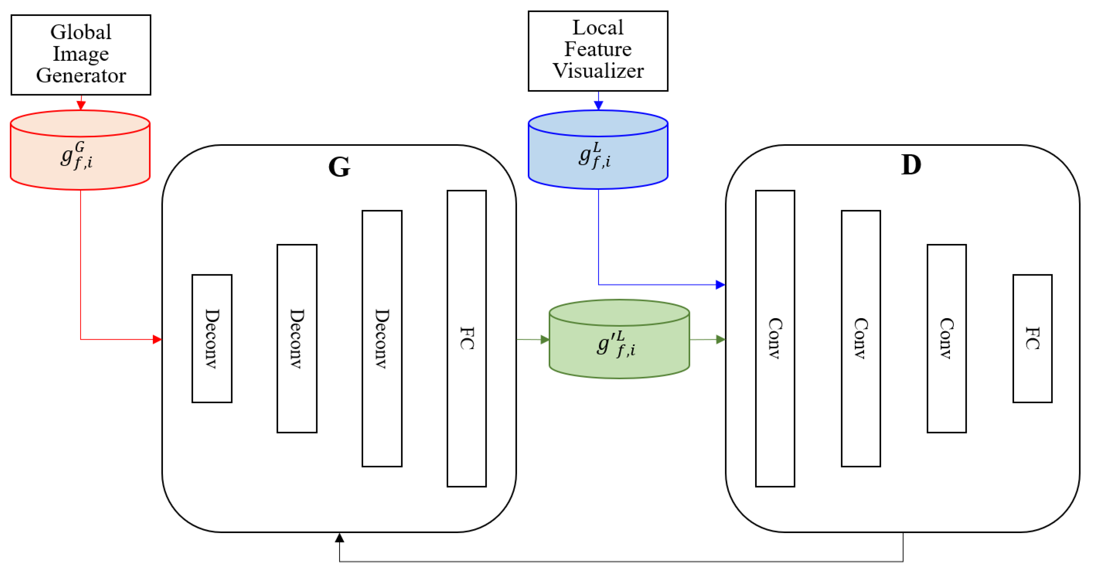
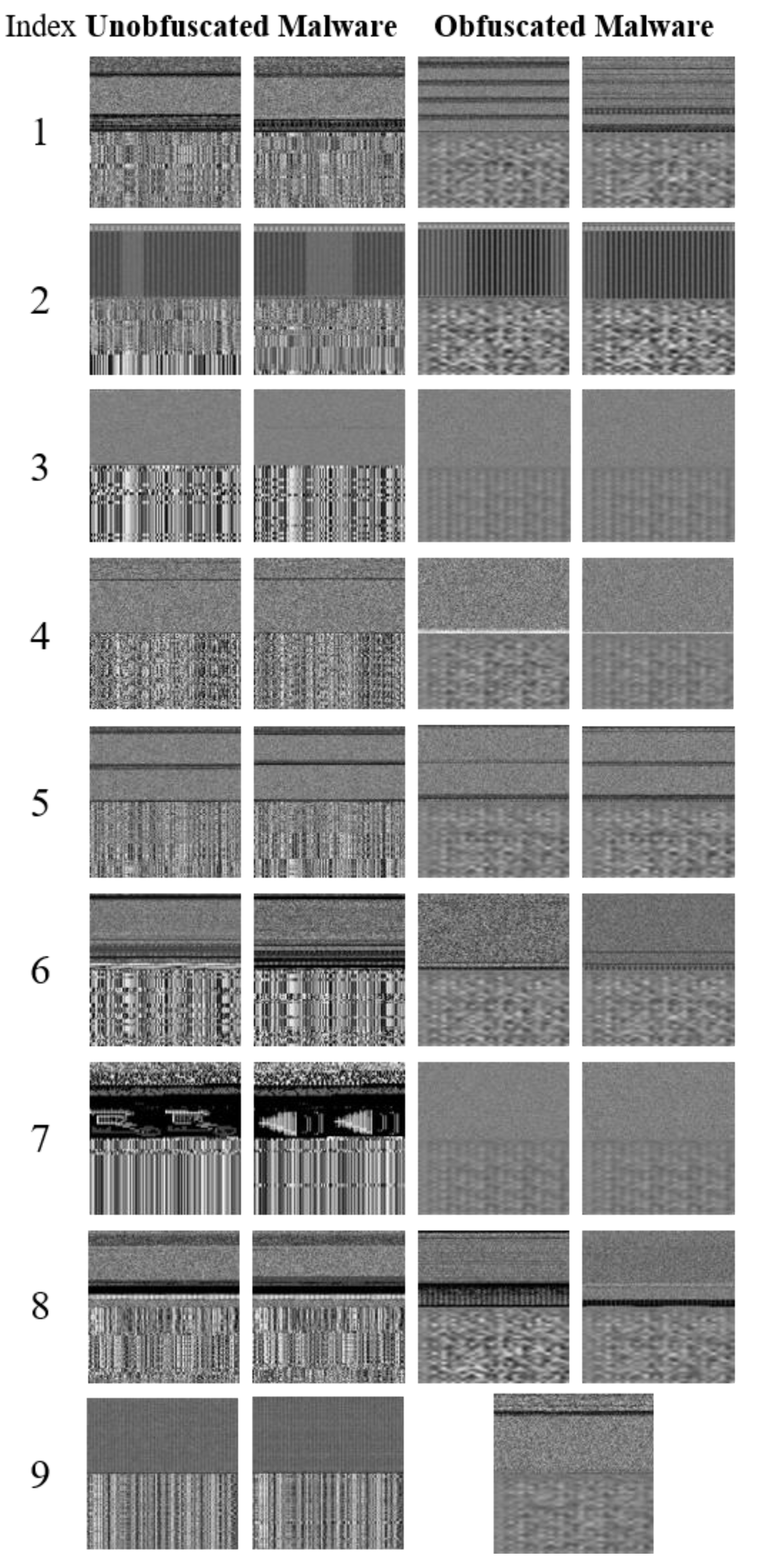
• Global image-based local feature visualization: A local feature visualization method based on a global image is proposed, for the first time, in this paper. The local images of obfuscated malware are created using a GAN based on the global images of obfuscated malware. It is difficult to identify obfuscated malware using text-based malware detection or classification methods. Through this method, the local features of obfuscated malware are simply generated. The generated local image is appropriate for malware classification because each malware family has unique patterns.
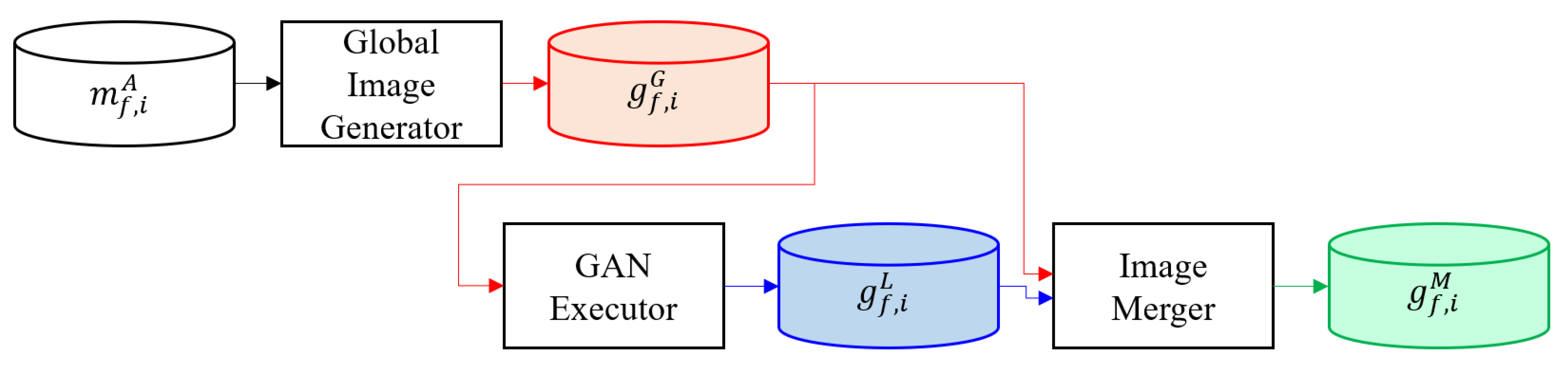
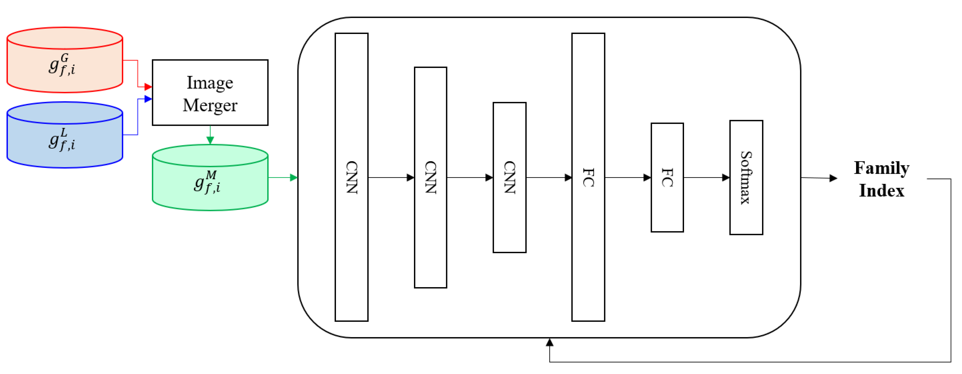
• Merged image-based malware classification: A global and local image merge method is proposed, for the first time, that uses global and local images in conjunction. When classifying the malware, small changes are detected using the local images of obfuscated and unobfuscated malware, and the overall structure is identified using the global images of obfuscated and unobfuscated malware.

In Section 2 of this paper, related work is overviewed and the background of the proposed method is discussed. In Section 3, the proposed method is presented in detail, and in Section 4, the proposed method is verified using a dataset that includes obfuscated and unobfuscated malware. In Section 5 and Section 6, the experimental results are analyzed and conclusions are stated, respectively.

2. Related Work

2.1. Dynamic and Static Analysis-Based Malware Detection and Classification Methods

Feng et al. [22] proposed a dynamic analysis framework called EnDroid that utilizes a feature selection algorithm to extract the behavior of malware and remove unnecessary features. Xue et al. [23] proposed a malware classification system based on probability scoring and machine learning called Malscore. Malscore uses a hybrid analysis method and sets the probability thresholds of static and dynamic analyses. It is resilient to obfuscation malware. Vinayakumara et al. [24] proposed an effective model using recurrent neural network (RNN) and long short-term memory (LSTM) to detect malware. LSTM, being effective when using big sequences, is more accurate than RNN. HaddadPajouh et al. [25] proposed a novel method to detect malware using RNN. They utilize a term frequency inverse document frequency (TFIDF) algorithm to select important features extracted from malware. Damodaran et al. [26] investigated static, dynamic, and hybrid analyses malware detection methods. They found that static analysis-based malware detection methods that utilize APIs can exhibit high accuracy. In contrast, static analysis-based malware detection methods utilizing opcode do not exhibit good performance when applied to certain malware families because the malware is obfuscated. In detecting or classifying malware, dynamic analysis methods generally exhibit high accuracy. However, they are more time consuming than static analysis methods.

2.2. Global Image-Based Malware Detection and Classification Methods

Nataraj [17] proposed a malware visualization method wherein binary information extracted from malware is divided into 8-bit units, and each 8-bit unit is used as one pixel. Because eight units of binary information can express values from 0 to 255, they are appropriate for use as pixels for grayscale images. After extracting textures from the existing global images, malware were accurately classified using k-nearest neighbors. Kancherla and Mukkamala [18] generated global images using the same method proposed by Nataraj [17]. They detected malware through a support vector machine using three features of the existing global images: intensity, wavelet, and gabor. However, because the global image-based malware detection methods proposed by Nataraj [17] and Kancherla and Mukkamala [18] have difficulty extracting binary information from obfuscated malware to generate global images, they also have difficulty detecting obfuscated malware. Gibert et al. [27] proposed a visualization method to classify obfuscated malware. Their proposed method generates a grayscale image utilizing every byte extracted from the malware. Then, three features—GIST, principal component, and Haralick—extracted from the malware are used to classify the malware.

2.3. Local Feature-Based Malware Detection and Classification Methods

Ni et al. [28] proposed a malware classification method that combines SimHash, a malware visualization technique, with a CNN. Their method creates grayscale images using SimHash based on the opcode extracted from the malware. They accurately classified malware based on the CNN; however, accurate experiments could not be performed owing to limitations of the experimental data. Fu et al. [20] proposed a malware classification method using local features along with the malware global image. They accurately classified malware using local features extracted from the code section, and texture and color features extracted from global images. However, the methods proposed by Ni et al. [28] and Fu et al. [20] cannot classify obfuscated malware accurately because it is difficult to extract the local features of obfuscated malware. Consequently, various local features, such as API, opcode, and dynamic link library (DLL), which represent the behavior of malware, cannot be considered. These disadvantages can lower classification accuracy.

In the methods proposed in this paper, local features are visualized based on global images to avoid the difficulty of extracting local features from obfuscated malware. The accuracy of malware classification is improved using the generated global and local images in conjunction.

3. Global Image-Based Local Feature Visualization, and Global and Local Image Merge Algorithm

In this section, the global image-based local feature visualization, and the global and local image merge methods are presented. The proposed method is divided into an input phase, a preprocessing phase, and a training and classification phase.

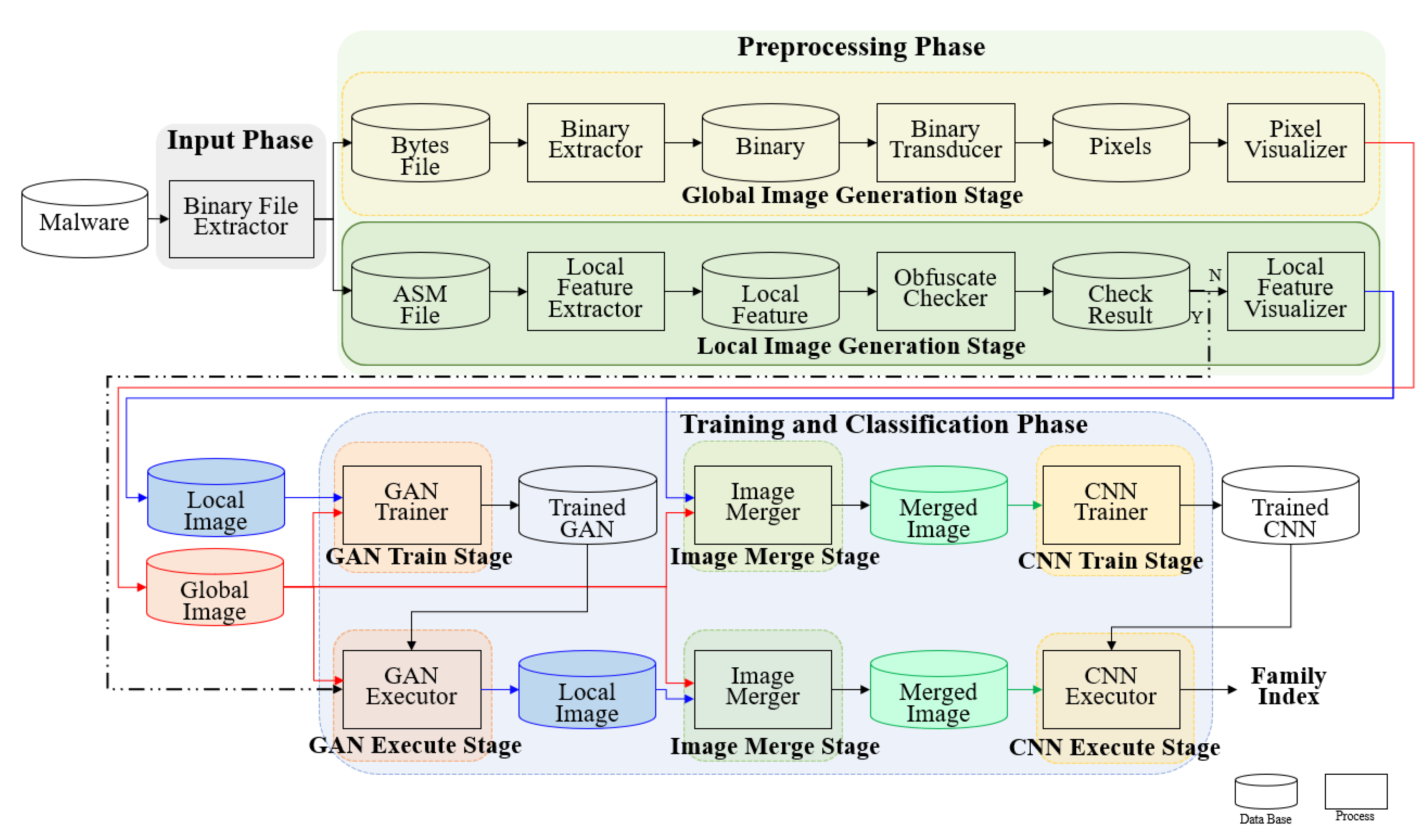
3.1. Overview of Proposed Method

Figure 1 gives an overview of the proposed method, which is divided into three phases: input, preprocessing, and training and classification. In the input phase, byte and assembly language source code (ASM) files are extracted from the malware samples using a disassembler. The binary file extractor receives the malware as input and outputs the ASM and byte files. These files are input to the global and local image generation stages, respectively.

In the preprocessing phase, global and local images of the malware are generated utilizing the features extracted from the malware. A global image and a local image are created from one malware. The preprocessing phase is divided into a global image generation stage and a local image generation stage. The global image, which includes all the information on the malware, is generated based on the binaries extracted from the malware. The binary extractor receives the bytes file as input and outputs binaries. The output binaries are converted into pixels using a binary transducer. Finally, the pixels are converted into a global image using a pixel visualizer. The local image contains local features such as API function and opcodes of the malware. In the local image generation stage, the local images are created based on the local features extracted from the malware. The local feature extractor receives the ASM file as input and outputs of the local features. The obfuscate checker receives the local features as input and checks for obfuscation. If the malware is obfuscated, the ASM file does not reveal the features. Therefore, the local feature visualizer and GAN trainer phases are skipped, and the GAN executor functions. If the malware is unobfuscated, a local image is created through the local feature visualizer using the extracted local features.

In the training and classification phases, the GAN model is trained and executed, the global and local images are merged, and the CNN model is trained and executed. The training and classification phase is divided into the GAN training, GAN execution, image merging, CNN training, and CNN execution stages. The GAN training and execution stages help generate a local image of the obfuscated malware. In the GAN training stage, the GAN model is trained; the GAN trainer receives the global and local images of unobfuscated malware as input, and outputs a trained GAN. In the GAN execution stage, a local image of the obfuscated malware is output through the trained GAN model utilizing the global image of the obfuscated malware. The GAN executor receives the global image of the obfuscated malware and the trained GAN as inputs, and outputs a local image of the obfuscated malware. The image merge stage merges the global and local images generated during the preprocessing phase. In the image merging stage, the global and local images of the unobfuscated and obfuscated malware are merged. The image merger receives the global and local images of the unobfuscated and obfuscated malware as inputs, and outputs a merged image. The CNN training and execution stages classify the malware using the merged image of the malware. In the CNN training stage, the CNN is trained using the merged image of the unobfuscated and obfuscated malware. The CNN trainer receives the merged image as input and outputs as a trained CNN. In the CNN execution stage, the unobfuscated and obfuscated malware are classified into families using the trained CNN. The CNN executor receives the merged images and trained CNN as inputs and outputs the family index of the unobfuscated and obfuscated malware. Because the family index is a number assigned to each malware family, each malware is classified under a family.

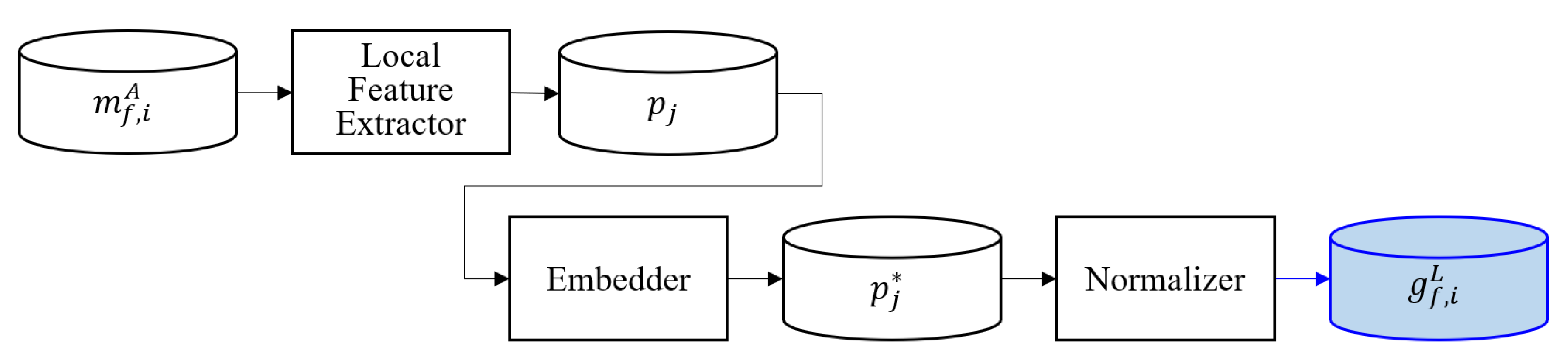
3.2. Input and Preprocessing Phases

In this paper, D denotes a database and $m_{f,i}$ the malware included in D. Therefore, D is considered a set of malware [$m_{f,1}$, $m_{f,2}$, …, $m_{f,i}$, …, $m_{f,\left|m_f\right|}$]. $m_{f,i}^U$ is the unobfuscated malware and $m_{f,i}^O$ is the obfuscated malware. $m_{f,i}$ is either $m_{f,i}^U$ or $m_{f,i}^O$. $m_{f,i}^A$ is the ASM file of malware and $m_{f,i}^B$ is the bytes file of malware. $G_{f,i}^g$ is the global image of malware. $p_j$ represents the local features extracted from $m_{f,i}^U$. $p_j^{*}$ represents the embedded local features. $g_{f,i}^L$ is the local image of $m_{f,i}^U$.

In the input phase, the binary file extractor receives $m_{f,i}$ as input and outputs $m_{f,i}^A$ and $m_{f,i}^B$. In the preprocessing phase, global images are generated using the malware image creation method proposed by Nataraj [17]. $g_{f,i}^g$ is created by extracting binary features from $m_{f,i}^B$. Figure 2 shows the local feature visualization process. The extracted ASM file is input into a local feature extractor that outputs $p_j$, which are embedded in an embedder. Next, $p_j^{*}$ are normalized using a normalizer. Finally, the normalizer outputs $g_{f,i}^L$.

3.3. Training and Classification Phase

In this section, the training and classification phase is introduced. This phase is divided into the GAN training and execution, global and local image merging, and CNN training and classification stages.

3.3.1. GAN Training and Execution Stage

In this paper, $g{\prime }_{f,i}^L$ is a fake local image created by GAN; and $\mathrm{G}$ and $\mathrm{D}$ are the generator and discriminator of GAN, respectively.

To visualize $p_j$ of $m_{f,i}^O$, the GAN is used, as shown in Figure 3. The GAN is composed of $\mathrm{G}$ and $\mathrm{D}$. $\mathrm{G}$ and $\mathrm{D}$ both comprise three CNN layers and one fully connected (FC) layer each. Because $p_j$ cannot be extracted from $m_{f,i}^O$, $g_{f,i}^L$ of $m_{f,i}^O$ is created using $g_{f,i}^G$ of $m_{f,i}^O$. Next, $g_{f,i}^G$ created from $m_{f,i}^U$ is input to $\mathrm{G}$, and $g_{f,i}^L$ of $m_{f,i}^U$ is input to $\mathrm{D}$ to train the GAN. $\mathrm{G}$ receives $g_{f,i}^G$ of $m_{f,i}^U$ as input and generates $g{\prime }_{f,i}^L$. $\mathrm{D}$ receives $g{\prime }_{f,i}^L$ generated by $\mathrm{G}$ as input and compares it to $g_{f,i}^L$ of $m_{f,i}^U$ to check if they are identical. Subsequently, $\mathrm{G}$ is trained by receiving the comparison result from $\mathrm{D}$.

Equation (1) shows the loss functions of $\mathrm{G}$ and $\mathrm{D}$. $Los{s}_D$ is the loss of $\mathrm{D}$ and $Los{s}_G$ is the loss of $\mathrm{G}$. $Los{s}_D$ is trained by maximizing the loss based on the result of $\mathrm{D}$. $\mathrm{G}$ is trained to optimize the loss using $Los{s}_D$ by considering the results of the discriminators:

$$\begin{gathered} Los{s}_D\left(D,G\right)= E_{g_{f,i}^L}\left[\log D\left(g_{f,i}^L\right)\right]+E_{g_{f,i}^G}\left[1-\log D\left(G\left(g_{f,i}^G \right)\right)\right], \\ Los{s}_G\left(D,G\right)= E_{g_{f,i}^G}\left[1-\log D\left(G\left(g_{f,i}^L\right)\right)\right]. \end{gathered}$$

(1)

Once training is completed, GAN receives $g_{f,i}^G$ of $m_{f,i}^O$ and outputs $g_{f,i}^L$ of $m_{f,i}^O$. All the generated $g_{f,i}^G$ and $g_{f,i}^L$ are reshaped because the size of each malware is different.

3.3.2. Global and Local Image Merging Stage

In this paper, $g_{f,i}^M$ is the merged image obtained utilizing $G_{f,i}^g$ and $g_{f,i}^L$. In the global image and local image merging stage, the created $g_{f,i}^G$ and $g_{f,i}^L$ are merged, as shown in Figure 4. $g_{f,i}^M$ of $g_{f,i}^G$ and $g_{f,i}^L$ is output using an image merger.

Algorithm 1 shows the image merge algorithm. $SIZE( )$ is a function that returns the size of the inputted value. ${\mathsf{\Omega }}_{f,i}$ is the two-dimensional array used to create $g_{f,i}^M$.

The image merge algorithm generates $g_{f,i}^M$ using $g_{f,i}^G$, $g_{f,i}^L$, and $p_j^{*}$. The row size of $g_{f,i}^M$ is the sum of the sizes of the functions $SIZE\left(g_{f,i}^G\right)$ and $SIZE\left(g_{f,i}^L\right)$. The column size of $g_{f,i}^M$ is equal to the size of $SIZE\left(p_j^{*}\right)$. Therefore, $g_{f,i}^M$ is created by sequentially extracting and storing the pixels of $g_{f,i}^G$ and $g_{f,i}^L$.

Algorithm 1 Local Feature Visualization Algorithm

1 FUNCTION ImageMerger ($g_{f,i}^G$, $g_{f,i}^L$, $p_j^{*}$)

2 OUTPUT

3 $g_{f,i}^M$// Merged image

4

5 BEGIN

6 ${\mathsf{\Omega }}_{f,i}$←2-Dimension matrix for merged image $g_{f,i}^M$

7 FOR Zero to $SIZE\left(g_{f,i}^M\right)$

8 FOR Zero to $SIZE\left(p_j^{*}\right)$

9 IF pixel from $g_{f,i}^G$:

10 ${\mathsf{\Omega }}_{f,i}\left(m,n\right)$←Extract pixel from global image $g_{f,i}^G$

11 ELSE:

12 ${\mathsf{\Omega }}_{f,i}\left(m,n\right)$←Extract pixel from local image $g_{f,i}^L$

13 END FOR

14 END FOR

15

16 END

3.3.3. CNN Training and Classification Stage

In the CNN training stage, CNN is trained, as shown in Figure 5, using $g_{f,i}^M$ of $m_{f,i}$ generated in the global and local image merging stage. The CNN is composed of three convolution layers, two FC layers, and one softmax layer. The trained CNN predicts the family index of $m_{f,i}$ utilizing $g_{f,i}^M$ of $m_{f,i}$. It receives $g_{f,i}^M$ that are not used for training as input and classifies $m_{f,i}$ into each malware family.

4. Experimental Evaluation

In the experiments conducted, the process and result of the global image-based local feature visualization method and the image merge method were extracted to verify the proposed method. The results of malware classification were then obtained.

4.1. Dataset and Experimental Environments

The Microsoft Malware Classification Challenge (BIG 2015) dataset was used to verify the proposed method [29,30]. This dataset comprises approximately 500 GB of data divided into training data and test data. These data consist of ASM and byte files extracted using the Interactive DisAssembler (IDA) tool. Because the test data in the dataset had no label information, all the training data were used.

Table 1. Total number of obfuscated and unobfuscated malware, by family, used in the experiments.

Family Index	Family Name	Obfuscated Malware	Unobfuscated Malware	Total Number
1	Ramnit	28	1513	1541
2	Lollipop	8	2470	2478
3	Kelihos_ver3	6	2936	2942
4	Vundo	28	447	475
5	Simda	8	34	42
6	Tracur	457	294	751
7	Kelihos_ver1	11	387	398
8	Obfuscator.ACY	58	1170	1228
9	Gatak	1	1012	1013

shows the total number of obfuscated and unobfuscated malware, segregated by family, used in the experiments. The family index is the index of each malware family, and the family name is the real name of the malware of each family. The total number of obfuscated malware is 605, and that of unobfuscated malware is 10,263. As is obvious, the number of obfuscated malware is lower than the number of unobfuscated malware. The total number of obfuscated and unobfuscated malware is 10,868.

Table 2. Parameters and values used in the experiments.

GAN		CNN
Parameter	Value	Parameter	Value
Batchsize	64	Batchsize	32
Imageshape	(32,32,1)	Imageshape	(256,256)
Learningrate	0.0002	Learningrate	0.0001
Epoch	10	Epoch	50
Filter_size	5 × 5	Filter_size	3 × 3
G_h0	4 × 4 × 128	conv1	128 × 128 × 32
G_h1	8 × 8 × 64	conv2	64 × 64 × 32
G_h2	16 × 16 × 32	conv3	32 × 32 × 64
G_h3	32 × 32 × 1	Fc1	128
D_h0	16 × 16 × 1	Fc2	9
D_h1	8 × 8 × 64
D_h2	4 × 4 × 128
D_h3	64 × 1

shows the parameters of the experiments. Batchsize is the number of images entered at one time. Imageshape is the image size that is input to the GAN and CNN. Because of the limitation of experimental environments, the parameter Imageshape of GAN was set to (32,32,1). Epoch is the number of trainings. Filter_size is the filter size of the convolution. G_h0, G_h1, and G_h2 are the sizes of the convolutional layer of the generator of GAN and G_h3 is the size of the FC layer of the generator of GAN. D_h0, D_h1, and D_h2 are the sizes of the deconvolutional layer of the discriminator of GAN, and D_h3 is the size of the FC layer of the discriminator of GAN. Conv1, conv2, and conv3 are the sizes of the convolutional layer of the CNN. Fc1 and Fc2 are the sizes of the FC layer of the CNN.

4.2. Global Image and Local Image Merging Results

Figure 6 shows the result of the global and local malware images merged using the proposed method. The global images generalized to a size of 256 × 128 were merged with the local images generalized to a size of 256 × 128. The merged image is a square of 256 × 256. In the merged images, the upper image is the global image and the lower image is the local image. The boundary between the two images is identified through a specific pattern of the global image and the local image. For example, in the image on the left of the unobfuscated malware shown in index 1, the top image with black horizontal lines is the global image, and the bottom image that looks like a mosaic is the local image. In the case of unobfuscated malware, the unique pattern of each family can be identified. The global images of the obfuscated malware family, numbers 4, 7, 8, and 9, show different patterns from those of the unobfuscated malware family. The local images of the obfuscated malware show similar patterns as those of the unobfuscated malware.

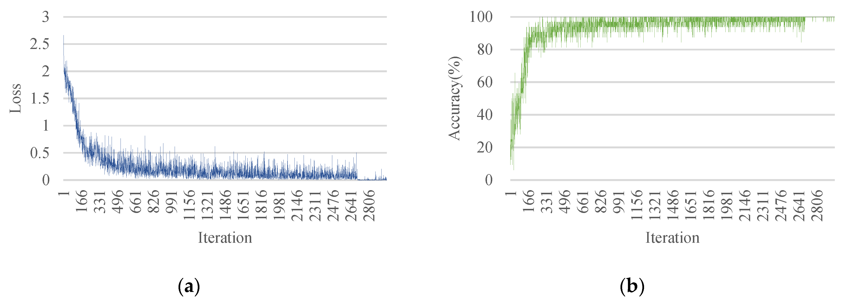
4.3. Results of Malware Classification

Figure 7 shows the loss and accuracy of the CNN model used to classify malware by applying the proposed method. The loss function represents the difference between the predicted and actual data. If the loss value is zero, the trained model predicts the data perfectly. Cross-entropy was used to train the GAN during the experiments. The train loss (Figure 7a) was measured as 2.6 in the first epoch. In the 28th epoch, the loss value converged to 0.0543. The train accuracy (Figure 7b) started from 15.6% in the first epoch and converged to 99.9% in the 28th epoch. The learning loss value was 0.0543 that converged to a low value; the learning accuracy was 99.9% that converged to a high value. This result shows that the CNN is well-trained using the proposed method.

Table 3. Comparison between proposed method and related work.

	Accuracy (%)	TFIDF (Top)	Used Image
Proposed	99.39	45	Merge Image
Proposed	99.47	50	Merge Image
Proposed	99.65	55	Merge Image
Proposed	99.56	60	Merge Image
Proposed	99.39	65	Merge Image
Jianwen Fu et al. [20]	97.47		Global Image, Local Feature
Ni et al. [22]	99.26		Local Feature
Nataraj [17]	98.00		Global Image
Kancherla and Mukkamala [18]	95.95		Global Image

shows the malware classification accuracy of each TFIDF classified using the proposed method. When the local image was created using the top 55 TFIDF, the accuracy was 99.65%. Fu et al. [20] proposed a malware classification method that utilizes global image and local features. Their method differs from the proposed method in that the proposed method uses global and local images while their method uses one global image and local feature (text) extracted from the malware. The accuracy of the proposed method is 2.18% higher than that of the method proposed by Fu et al. [20] Ni et al. [22] proposed a method that visualizes local features to classify the malware. They used the same dataset as the one used in our approach; however, they did not use obfuscated malware. Although the proposed method utilizes all datasets, including obfuscated malware, it derives a higher accuracy of 0.39% than the method proposed by Ni et al. [22] Nataraj [17] and Kancherla and Mukkamala [18] proposed malware detection and classification methods using the global image of the malware. Compared to our method, the only difference is the feature extraction method used in these methods. The proposed method shows a higher accuracy of 1.65% and 3.7% compared to the methods proposed by Nataraj [17] and Kancherla and Mukkamala [18], respectively.

5. Discussion

5.1. Results of Obfuscated and Unobfuscated Malware Classification

In the case of unobfuscated malware, 1024 out of a total of 1024 malwares were classified into each family, showing an accuracy of 100%. In the case of obfuscated malware, 124 out of 128 malware instances were classified into each family, showing an accuracy of 96.87%. The local images of obfuscated malware were created based on the global images of obfuscated malware using GAN. However, the created local images were inaccurate compared to the local images of the unobfuscated malware. The patterns of each malware family are important because they are utilized when classifying the malware. However, the unique patterns of each obfuscated malware family were not clearly derived. Therefore, the classification accuracy of obfuscated malware is lower than the classification accuracy of unobfuscated malware.

Table 4. False positive, false negative, precision, and recall of obfuscated malware.

True Positive	True Negative	False Positive	False Negative	Precision	Recall	F-1 Score
13.77	113.33	0.44	0.44	0.96	0.96	0.96

shows the true positive, true negative, false positive, false negative, precision, recall, and F-1 score of obfuscated malware. A low value than the value of unobfuscated malware was obtained because the number of obfuscated malware was imbalanced and small. In the case of 2, 3, 5, and 9, each family has each number of malware only 8, 6, 8, and 1 has obfuscated malware. The value of precision, recall, and F-1 were the same because of false positive and false negative were the same.

Table 5. Comparison between proposed method and of Fu et al.’s method.

	Obfuscated Malware (%)	Unobfuscated Malware (%)
Proposed Method	97	100
Fu et al. [20]	99	98

shows the accuracies of the proposed method and the method of Fu et al. [20] The approach of Fu et al. [20] was validated by the method utilizing 15 families of malwares. By the confusion matrix provided by Fu et al. [20], the accuracy of obfuscated and non-obfuscated malwares were derived. The provided confusion matrix included information about the accuracy of 15 families of malwares. If the “obfuscated” was included in a certain family name, the corresponding malware family was obfuscated malware. The approach of Fu et al. [20] has the accuracy for obfuscated malwares by 99%. This result is approximately 2% higher than that of the proposed method. However, their result was obtained using twice the number of obfuscated malwares as that used with the proposed method. For the unobfuscated malware, the accuracy of the proposed method is approximately 2% higher than that of Fu et al. [20] This result verifies that merging global image and local images is more effective than using global image and local feature.

5.2. Comparison between Proposed Method and Previous Methods

Kim et al. [21] proposed a transferred deep-convolutional GAN (tDCGAN) to detect malware, including zero-day attacks. tDCGAN generates a fake malware similar to the real malware and the detector learns the fake malware generated. It can then detect variant malware—the real malware. However, because the visualization of the obfuscated malware is difficult, there is a limitation on the experimental data. The experimental data used in this paper are the same as those used by Kim et al. [21] However, approximately a 4% higher accuracy was obtained without limitation in the experimental data. Furthermore, by visualizing the local features of the global image of the malware using the global image-based local feature visualization method, the actual behavior of the malware is considered.

6. Conclusions

In this paper, two methods, global image-based local feature visualization and global and local image merge, were proposed. First, a global image of obfuscated and unobfuscated malware and a local image of unobfuscated malware are generated in the preprocessing phase. Second, the GAN is trained using the global and local images of unobfuscated malware generated in the preprocessing phase. Third, a local image of obfuscated malware is generated using the trained GAN. Fourth, the global and local images of unobfuscated and obfuscated malware created using the global and local image merge technique are merged. Fifth, the CNN is trained using the merged images of the unobfuscated and obfuscated malware. Sixth, the unobfuscated and obfuscated malware are classified into different families using the trained CNN. Gibert et al. [28] obtained an accuracy of 97.5% using the global image of malware with the same dataset used in this paper. Our approach is 2.15% more accurate than the method proposed by Gibert et al. [28] Fu et al. [20] achieved an accuracy of 97.47% using the global image and local feature (text) of malware. The proposed method is 2.18% more accurate than that proposed by Fu et al. [20].

In future work, an RGB-based malware visualization technique will be investigated to improve the proposed method. The local features extracted from malware will be pixelated, which may reduce the malware detection time. In addition, methods to reduce various processes by merging the pixelated local features with the global images will be studied.

References

1. Liu, Y.S.; Lai, Y.K.; Wang, Z.H.; Yan, H.B. A New Learning Approach to Malware Classification using Discriminative Feature Extraction. IEEE Access 2019, 7, 13015–13023. [Google Scholar] [CrossRef]
2. Guillén, J.H.; del Rey, A.M.; Casado-Vara, R. Security Countermeasures of a SCIRAS Model for Advanced Malware Propagation. IEEE Access 2019, 7, 135472–135478. [Google Scholar] [CrossRef]
3. Nissim, N.; Cohen, A.; Wu, J.; Lanzi, A.; Rokach, L.; Elovici, Y.; Giles, L. Sec-Lib: Protecting Scholarly Digital Libraries From Infected Papers Using Active Machine Learning Framework. IEEE Access 2019, 7, 110050–110073. [Google Scholar] [CrossRef]
4. Mahboubi, A.; Camtepe, S.; Morarji, H. A Study on Formal Methods to Generalize Heterogeneous Mobile Malware Propagation and Their Impacts. IEEE Access 2017, 5, 27740–27756. [Google Scholar] [CrossRef]
5. Belaoued, M.; Derhab, A.; Mazouzi, S.; Khan, F.A. MACoMal: A Multi-Agent Based Collaborative Mechanism for Anti-Malware Assistance. IEEE Access 2020, 8, 14329–14343. [Google Scholar] [CrossRef]
6. Bilar, D. Opcodes as Predictor for Malware. Int. J. Electron. Secur. Digit. Forensics 2007, 1, 156–168. [Google Scholar] [CrossRef]
7. Albladi, S.; Weir, G.R. User Characteristics that Influence Judgment of Social Engineering Attacks in Social Networks. Hum. Cent. Comput. Inf. Sci. 2018, 8, 1–24. [Google Scholar] [CrossRef]
8. Gandotra, E.; Bansal, D.; Sofat, S. Malware Analysis and Classification: A Survey. J. Inf. Secur. 2014, 5, 56–64. [Google Scholar] [CrossRef] [Green Version]
9. Santos, I.; Brezo, F.; Ugarte-Pedrero, X.; Bringas, P.G. Opcode Sequences as Representation of Executables for Data-mining-based Unknown Malware Detection. Inf. Sci. 2013, 231, 64–82. [Google Scholar] [CrossRef]
10. Souri, A.; Hosseini, R.A. State-of-the-Art Survey of Malware Detection Approaches using Data Mining Techniques. Hum. Cent. Comput. Inf. Sci. 2018, 8, 1–22. [Google Scholar] [CrossRef]
11. Vinayakumar, R.; Alazab, M.; Soman, K.P.; Poornachandran, P.; Venkatraman, S. Robust Intelligent Malware Detection using Deep Learning. IEEE Access 2019, 7, 46717–46738. [Google Scholar] [CrossRef]
12. Homayoun, S.; Dehghantanha, A.; Ahmadzadeh, M.; Hashemi, S.; Khayami, R. Know Abnormal, Find Evil: Frequent Pattern Mining for Ransomware Threat Hunting and Intelligence. IEEE Trans. Emerg. Top. Comput. 2017, 8, 341–351. [Google Scholar] [CrossRef]
13. Zhao, B.; Han, J.; Meng, X. A Malware Detection System Based on Intermediate Language. In Proceedings of the 2017 4th International Conference on Systems and Informatics (ICSAI), Hangzhou, China, 11–13 November 2017; pp. 824–830. [Google Scholar]
14. Tang, M.; Qian, Q. Dynamic API Call Sequence Visualisation for Malware Classification. IET Inf. Secur. 2018, 13, 367–377. [Google Scholar] [CrossRef]
15. Zhang, H.; Xiao, X.; Mercaldo, F.; Ni, S.; Martinelli, F.; Sangaiah, A.K. Classification of Ransomware Families with Machine Learning based on N-gram of Opcodes. Future Gener. Comput. Syst. 2019, 90, 211–221. [Google Scholar] [CrossRef]
16. Kim, J.; Kim, H.; Kim, I.K. Cyber Genome Technology for Countering Malware. Electron. Telecommun. Trends 2015, 30, 118–128. [Google Scholar] [CrossRef]
17. Nataraj, L. Malware Images: Visualization and Automatic Classification. In Proceedings of the 8th International Symposium on Visualization for Cyber Security, ACM, Pittsburgh, PA, USA, 20 July 2011; pp. 1–7. [Google Scholar]
18. Kancherla, K.; Mukkamala, S. Image Visualization based Malware Detection. In Proceedings of the 2013 IEEE Symposium on Computational Intelligence in Cyber Security (CICS), Singapore, 16–19 April 2013; pp. 40–44. [Google Scholar]
19. Yang, H.; Li, S.; Wu, X.; Lu, H.; Han, W. A Novel Solutions for Malicious Code Detection and Family Clustering Based on Machine Learning. IEEE Access 2019, 7, 148853–148860. [Google Scholar] [CrossRef]
20. Fu, J.; Xue, J.; Wang, Y.; Liu, Z.; Shan, C. Malware Visualization for Fine-grained Classification. IEEE Access 2018, 6, 14510–14523. [Google Scholar] [CrossRef]
21. Kim, J.Y.; Bu, S.J.; Cho, S.B. Zero-day Malware Detection using Transferred Generative Adversarial Networks based on Deep Autoencoders. Inf. Sci. 2018, 460, 83–102. [Google Scholar] [CrossRef]
22. Feng, P.; Ma, J.; Sun, C.; Xu, X.; Ma, Y. A Novel Dynamic Android Malware Detection System with Ensemble Learning. IEEE Access 2018, 6, 30996–31011. [Google Scholar] [CrossRef]
23. Xue, D.; Li, J.; Lv, T.; Wu, W.; Wang, J. Malware Classification Using Probability Scoring and Machine Learning. IEEE Access 2019, 7, 91641–91656. [Google Scholar] [CrossRef]
24. Vinayakumar, R.; Soman, K.P.; Poornachandran, P.; Sachin Kumar, S. Detecting Android Malware using Long Short-Term Memory (LSTM). J. Intell. Fuzzy Syst. 2018, 34, 1277–1288. [Google Scholar] [CrossRef]
25. HaddadPajouh, H.; Dehghantanha, A.; Khayami, R.; Choo, K.K.R. A Deep Recurrent Neural Network based Approach for Internet of Things Malware Threat Hunting. Futur. Gener. Comput. Syst. 2018, 85, 88–96. [Google Scholar] [CrossRef]
26. Damodaran, A.; Di, F.T.; Visaggio, C.A.; Austin, T.H.; Stamp, M. A Comparison of Static, Dynamic, and Hybrid Analysis for Malware Detection. J. Comput. Virol. Hacking Tech. 2015, 13, 1–12. [Google Scholar] [CrossRef]
27. Gibert, D.; Mateu, C.; Planes, J.; Vicens, R. Using Convolutional Neural Networks for Classification of Malware Represented as Images. J. Comput. Virol. Hacking Tech. 2018, 15, 15–28. [Google Scholar] [CrossRef] [Green Version]
28. Ni, S.; Qian, Q.; Zhang, R. Malware Identification using Visualization Images and Deep Learning. Comput. Secur. 2018, 77, 871–885. [Google Scholar] [CrossRef]
29. Kalash, M.; Rochan, M.; Mohammed, N.; Bruce, N.D.; Wang, Y.; Iqbal, F. Malware Classification with Deep Convolutional Neural Networks. In Proceedings of the 2018 9th IFIP International Conference on New Technologies, Mobility and Security (NTMS), Paris, France, 26–28 February 2018; pp. 1–5. [Google Scholar]
30. Ronen, R.; Radu, M.; Feuerstein, C.; Yom-Tov, E.; Ahmadi, M. Microsoft Malware Classification Challenge. arXiv 2018, arXiv:1802.10135. [Google Scholar]
Figure 1. Overview of the proposed method.
Applsci 10 07585 g001
Figure 2. Local feature visualization process.
Applsci 10 07585 g002
Figure 3. General adversarial network (GAN) training process. Deconv is deconvolution, Conv is convolution and FC is fully connected.
Applsci 10 07585 g003
Figure 4. Global image and local image merging process.
Applsci 10 07585 g004
Figure 5. Convolutional neural network (CNN) training process.
Applsci 10 07585 g005
Figure 6. Merge results of global and local images.
Applsci 10 07585 g006
Figure 7. CNN training results: (a) The blue line shows the loss value of trained CNN; (b) The green line shows the accuracy of trained CNN.
Applsci 10 07585 g007