Evaluation of RGB-D Multi-Camera Pose Estimation for 3D Reconstruction

Abstract

Advances in visual sensor devices and computing power are revolutionising the interaction of robots with their environment. Cameras that capture depth information along with a common colour image play a significant role. These devices are cheap, small, and fairly precise. The information provided, particularly point clouds, can be generated in a virtual computing environment, providing complete 3D information for applications. However, off-the-shelf cameras often have a limited field of view, both on the horizontal and vertical axis. In larger environments, it is therefore often necessary to combine information from several cameras or positions. To concatenate multiple point clouds and generate the complete environment information, the pose of each camera must be known in the outer scene, i.e., they must reference a common coordinate system. To achieve this, a coordinate system must be defined, and then every device must be positioned according to this coordinate system. For cameras, a calibration can be performed to find its pose in relation to this coordinate system. Several calibration methods have been proposed to solve this challenge, ranging from structured objects such as chessboards to features in the environment. In this study, we investigate how three different pose estimation methods for multi-camera perspectives perform when reconstructing a scene in 3D. We evaluate the usage of a charuco cube, a double-sided charuco board, and a robot’s tool centre point (TCP) position in a real usage case, where precision is a key point for the system. We define a methodology to identify the points in the 3D space and measure the root-mean-square error (RMSE) based on the Euclidean distance of the actual point to a generated ground-truth point. The reconstruction carried out using the robot’s TCP position produced the best result, followed by the charuco cuboid; the double-sided angled charuco board exhibited the worst performance.

1. Introduction

The idea and use of 3D imaging dates back to the 19th century, and laser scanning to the 1960s [1], but only recently has it been capable of revolutionising the interaction between robots, the environment and humans. Many advances in computational power, sensor precision and affordability have made this possible [2,3,4].

The recent development of RGB-D cameras has provided visual sensor devices capable of generating pixel-wise depth information, together with a colour image. The technology behind these cameras has been constantly improving, with developers working to reduce noise and increase precision, e.g., Microsoft Kinect Azure and Intel RealSense L515 and D455 [3].

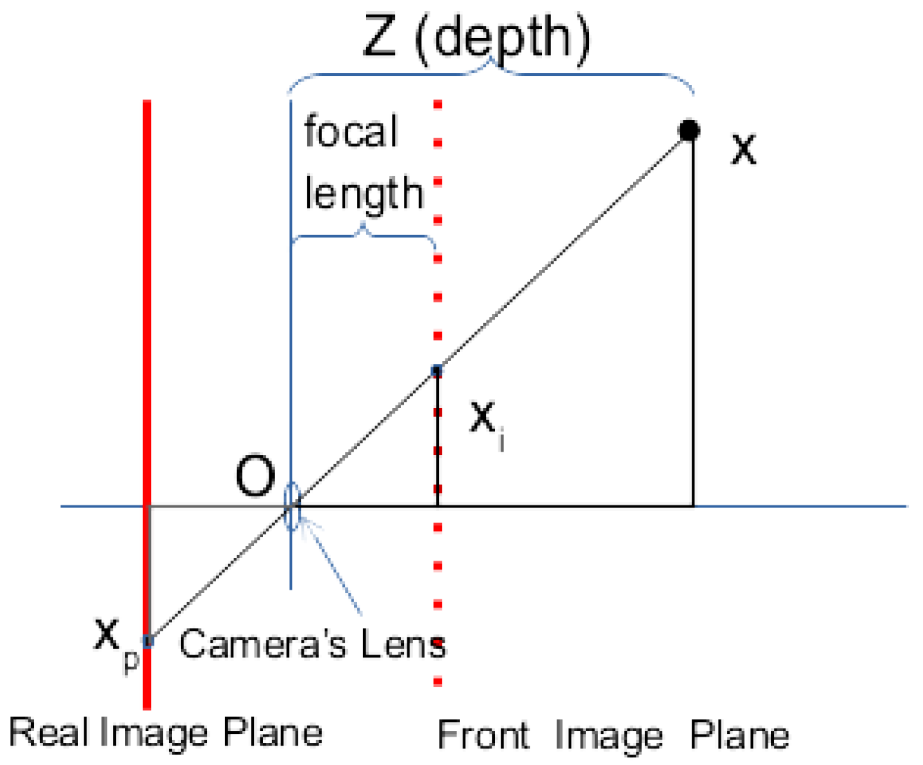
The depth information from those devices can be used to generate a three-dimensional projection of the captured object. Understanding the well-known pinhole camera model [5] is important to understand how the reprojection works, and how it is affected by noise in the depth data.

The model describes the transformation from the 3D world to the 2D image plane, as shown in Figure 1 and in the Equation (1) [6]. It can also be used to calculate the inverse path for reprojecting from 2D to 3D.

Equation (1) has two matrices: one for the intrinsic parameters and another for the extrinsic parameters. The first contains the camera’s internal parameters, which are constant for each camera. The second describes where the camera is in the world, i.e., the pose of the camera in relation to an origin coordinate system.

The direction vector of the ray from the camera projection centre can be found using these parameters, but the length of the vector cannot. This information is lost in the conversion from 3D to 2D. However, when using an RGB-D camera this information is saved, as a depth that determines where the point lies in the world. The set of points reprojected from these data is called a point cloud.

Other parameters that are important for reprojection are the distortion coefficients which are used to correct the radial and tangential distortions of the lens [7]. In this work, the FRAMOS Industrial Depth Camera D415e, which was built with Intel^® RealSense™ technology, was used. The Intel^® RealSense module claims to have no lens distortions [8,9].

$$s\left[\begin{array}{c}u\\ v\\ 1\end{array}\right]=\underset{\mathrm{intrinsic}}{\underbrace{\left[\begin{array}{ccc}{f}_x& 0& c_x\\ 0& f_y& c_y\\ 0& 0& 1\end{array}\right]}}\underset{\mathrm{extrinsic}}{\underbrace{\left[\begin{array}{cccc}{r}_{11}& r_{12}& r_{13}& t_1\\ r_{21}& r_{22}& r_{23}& t_2\\ r_{31}& r_{32}& r_{33}& t_3\end{array}\right]}}\left[\begin{array}{c}X\\ Y\\ Z\\ 1\end{array}\right]$$

(1)

The intrinsic parameters of a camera are normally represented as a 3 × 3 matrix, as shown in Equation (2).

$$K=\left[\begin{array}{ccc}{f}_x& 0& c_x\\ 0& f_y& c_y\\ 0& 0& 1\end{array}\right]$$

(2)

where $f_x$ and $f_y$ are the focal lengths in the x and y directions, respectively. Furthermore, $c_x$ and $c_y$ are the optical centres of the image plane, shown as a solid red line in Figure 1.

As illustrated in Figure 1, the focal length is the distance from the camera lens to the image plane; since the pixel is not necessarily square, the focal length is divided by the pixel size in x and y, resulting in the variables $f_x$ and $f_y$, respectively, expressing the values in pixels.

The extrinsic parameters are typically represented by a homogeneous transformation matrix, shown in Equation (3), and this was well explained by Briot and Khalil (2015) [10]. This contains the rotation matrix $R_{3\times 3}$ and the translation vector $T_{3\times 1}$, representing the camera’s transformation in relation to the origin of the reference coordinate system in the desired scene.

$$D=\left[\begin{array}{cc}{R}_{3\times 3}& T_{3\times 1}\\ 0_{1\times 3}& 1\end{array}\right]$$

(3)

The distortion coefficients are the parameters used to describe the radial and the tangential distortion. They are represented as $k_n$ and $p_n$, respectively. The most notable distortion model is the Brown–Conrady model [11].

The term calibration normally refers to methods of estimating the intrinsic parameters, distortion coefficients and extrinsic parameters.

Quaternions are another way to express rotations in the three-dimensional vector space. This method has a compact representation and has some mathematical advantages [12,13]. It is commonly used by the robotics industry because it is more mathematically stable and avoids the gimbal lock phenomenon, where two axes align and prevent the rotation in one dimension.

The robotic arm used in this work, the ABB IRB 4600, uses quaternions for the orientation of its TCP. Equation (4) [14] shows the conversion method from quaternions to Euler angles used in the homogeneous transformation matrix which was used in this work.

$$\left[\begin{array}{c}\varphi \\ \theta \\ \psi \end{array}\right]=\left[\begin{array}{c}\mathrm{atan}2(2(q_0{q}_1+q_2{q}_3),1-2(q_1^2+q_2^2))\\ \mathrm{asin}\left(2(q_0{q}_2-q_3{q}_1)\right)\\ \mathrm{atan}2(2(q_0{q}_3+q_1{q}_2),1-2(q_2^2+q_3^2))\end{array}\right]$$

(4)

1.1. Point Cloud

Reprojecting the points in 3D using the intrinsic parameters in a pinhole model, as shown in Equation (1), with no distortion is carried out according to Equations (5)–(7). For an RGB-D device, Z is the depth information extracted from the depth frame, x is the column index and y is the row index. In these equations, a point is a 3D structure with $(x,y,z)$ data representing a point in the camera’s coordinate frame.

$$point.z=Z;$$

(5)

$$point.x=\left(\right(X-cx)/fx)\ast Z;$$

(6)

$$point.y=\left(\right(X-cy)/fy)\ast Z;$$

(7)

The origin of the coordinate system for each point cloud is one sensor of the camera, in this case, the left infrared sensor. To reconstruct the scene from multiple cameras or perspectives, the camera’s positionin the scene, i.e., the global coordinate system, must be known.

The global coordinate system’s origin is chosen according to the task. It can be the optical centre of one of the camera’s sensors, for example. In this work, the chosen origin was the base coordinate system of an ABB IRB 4600 robot [15].

1.2. Related Work

The problem of scene reconstruction has been well studied in different scenarios. To solve the challenge of registering two or more point clouds together, the six degrees of freedom (DoF) transformation between them has to be found. This can be calculated using the point clouds by either selecting the matching points manually or using algorithms to find possible matching points. Another method is to calculate a known position for the sensors.

Chen and Medioni [16] and Besl and McKay [17] proposed one of the most widely used algorithms for the registration of 3D shapes, the iterative closest point (ICP). It tries to find the best match between the point clouds by finding the closest points from one point cloud to the other, then it determines the transformation matrix that minimises the distance between the points, and finally, it iterates until it converges. Due to fact that it relies on the data association of the points between point clouds, a good overlap is necessary for convergence.

Wang and Solomon [18] proposed a replacement of ICP called the deep closest point (DCP) method, which uses a three-step approach, first embedding the point clouds into a common space, then capturing co-contextual information in an attention-based module and finally using singular value decomposition to find the transformation matrix.

Aoki et al. [19] used the Pointnet [20] method with the Lukas and Kanade (LK) [21] algorithm to solve the registration problem.

Other methods include that of Stoyanov et al. [22], who used a three-dimensional normal distribution transform representation of the distance between the models, followed by a Newton optimisation, and that of Zhan et al. [23], who proposed an algorithm based on normal vector and particle swarm optimisation. These methods all rely on having a sufficient overlap between the point clouds to solve the problem. Moreover, these methods tend to be slow.

Performing an estimation of the position of the sensorprovides a more reliable transformation for the point clouds. Initially, work on camera calibration was focused on finding the intrinsic parameters of a single camera. Zhang [24] was the first to propose the solution to this challenge using a chessboard pattern, i.e., a planar target, through least-square approximation.

With the intrinsic parameters, in theory, it would be possible to calculate the pose of the camera with four coplanar points that are not collinear, but Schweighofer and Axel [25], discussing pose ambiguities, proved that two local minima exist, and proposed an algorithm to solve this problem.

Fiducial markers became popular for camera pose estimations, and several markers have been proposed, including point-based [26], circle-based [27], and square-based [28,29] markers, which can determine the pose using the four corners and have the ID in the middle of the marker.

Garrido-Jurado et al. [28] proposed a system with configurable marker dictionaries, specially designed for camera localization. The authors developed a marker generator, as well as an automatic detection algorithm. These ArUco markers form the basis of the charuco board used in this work.

Other publications have proposed ways to solve the problem of pose estimation using an arbitrary scene with texture [30,31,32]. These are not relevant to this project, since it was designed in a contained environment.

In this work, we propose and carry out a novel evaluation method for multiple camera perspectives. We used a charuco to identify and label the points on which the metrics were based, and calculated the errors of three different methods in order to carry out the transformation of the cameras to the global coordinate system.

2. Materials and Methods

This investigation was part of two projects called Meatable [33] and RoButcher (https://robutcher.eu, accessed on 15 February 2022). The projects involved researching the design and robotisation of a cell to process pig carcasses, called the Meat Factory Cell, and proposing a significant deviation from existing meat processing practices. The process was briefly described by Alvseike et al. (2018) [34,35]. The projects defined constraints on the data captured due to the specific data configuration of the scene and the application requirements.

Due to the inherent characteristics of the projects, precision was a key aspect of the system; otherwise, the cutting and manipulation of carcasses would be unsatisfactory or ineffective (e.g., the robot could cut too deep into the carcass, or not cut it at all).

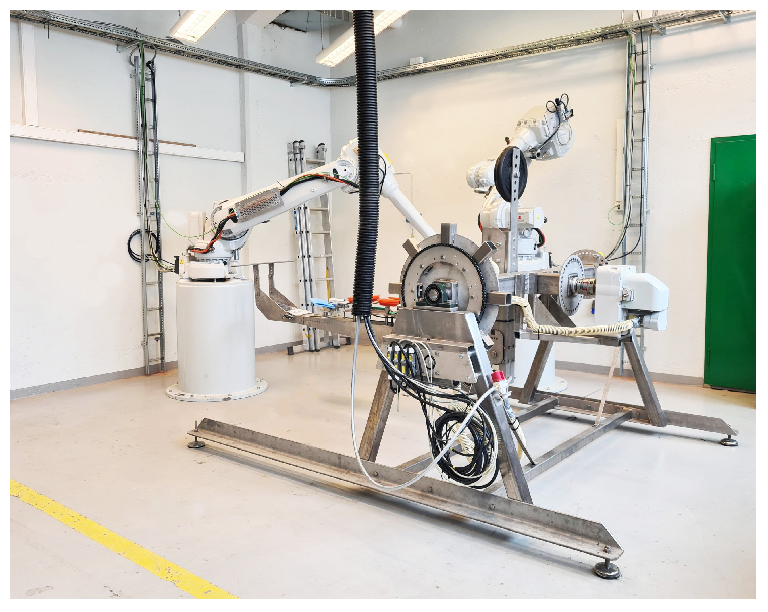
For these projects, a bespoke machine called a carcass handling unit (CHU) was used, as shown in Figure 2. Its function was to grip a pig’s carcass and present it to the robot, which would perform automated cutting to segment or dissect the parts.

The robot needed to have a complete understanding of the environment in the 3D space. However, the camera had a limited angle of view. To solve this constraint, multiple camera perspectives had to be transformed to obtain a complete view of the scene.

The robotic arm had a camera attached to the tool centre point (TCP), as illustrated in Figure 3, to capture the data. It cycled the camera to six positions around the CHU, with two on the right, two on top, and two on the left side. With this configuration, almost 360° of the scene could be captured.

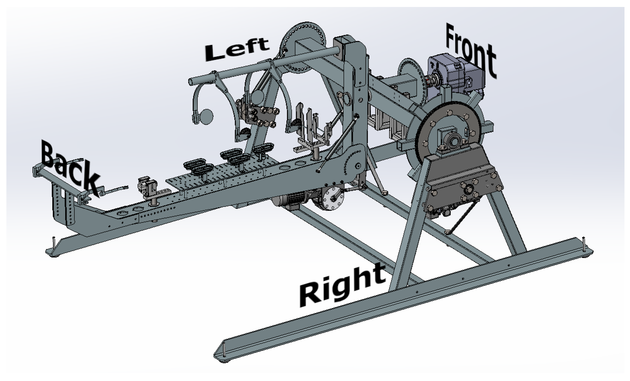
The cameras are referred to as left/right/up and front/back. The left/right is defined in relation to the CHU, not to the pig, which can be rotated once grabbed by the CHU. TThe left, right, front, and back sides of the CHU were defined as shown in Figure 4.

The FRAMOS D415e has 3 image sensors (2 infrared (IR) and 1 RGB) and one IR laser projector. It calculates depth based on the disparity between the two IR sensors. Furthermore, it is stated by the documentation that the infrared cameras have no distortion; hence, all the distortion coefficients are $0.0$ [9]. Furthermore, the cameras come from the factory calibrated with intrinsic parameters recorded in the memory and can be easily read using the appropriate Intel RealSense SDK library.

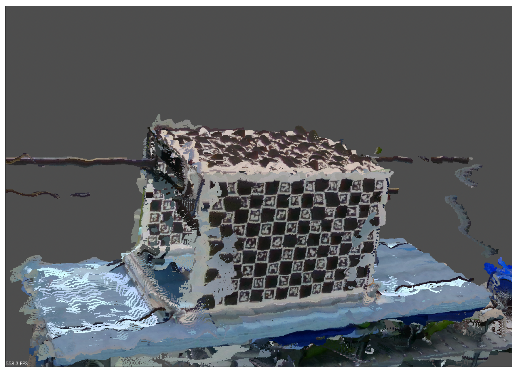
The Intel RealSense D415 was evaluated in regard to its the accuracy, performance, and precision by Lourenco and Araujo [36], with an RMSE accuracy distance for an analysis of 100 images of $0.07927$, an average failed points ratio of $0.5414\%$, and average outliers ($\pm 10$ cm) of $0.0667$%, measured at 1 m. The repetitive pattern of the board also prejudices the depth calculation, and consequentially the point cloud, as illustrated in Figure 5.

The data are recorded in a bag file (http://wiki.ros.org/Bags, accessed on 1 February 2022) using the SDK. The bagfile is a container file that contains the image and the depth frame, the intrinsic parameters for both sensors, and metadata information. These data are used to extract the parameters needed to execute the calibration.

The file-naming conventions used in the work used camera positions numbered from 0 to 5, and the sequential take number, with the following relation to the CHU:

• Left/Front: Cam 0
• Left/Back: Cam 1
• Up/Back: Cam 2
• Up/Front: Cam 3
• Right/Front: Cam 4
• Right/Back: Cam 5

2.1. Evaluation Metrics

To quantify the quality of the reconstruction in each method, the root-mean-square error (RMSE), shown in Equation (8), was used. The error used in the RMSE calculation was the Euclidean distance in three-dimensional space ${\mathbb{R}}^3$, and it was calculated after reprojecting the points in the point cloud, as shown in Equation (9).

$$rmse=\sqrt{\frac{{\displaystyle \sum _{i=0}^n}erro{r}^2}{n}}$$

(8)

$$error=\sqrt{{(x_o-x_r)}^2+{(y_o-y_r)}^2+{(z_o-z_r)}^2}$$

(9)

The depth information received from the camera was able to have an error of 2%, thus increasing the RMSE. However, as this affected all methods similarly, it did not interfere with the final comparison.

To measure the distance between the correspondents points, these points must be known, i.e, which point in one point cloud should match which point in the other point cloud. Since the point cloud from the RGB-D device did not contain information enabling us to identify which point was which, a method was proposed to label some points.

In this work we used OpenCV [37], as it is a stable and robust library for computer vision. ArUco markers were used as fiducial markers and a charuco board was used as the pattern board for the pose estimation, as proposed by Garrido et al. (2014) [28].

The ArUco module in OpenCV has all the necessary functions for pose estimation using the implemented charuco board [38].

2.2. Labelling Points

The method used to identify and label the points in order to enable error calculation was based on the unique ID of each ArUco marker. Each ID and the corners of the marker could be found on the board during the pose estimation process, as shown in Figure 6.

Equation (10) shows the calculation of the point label values at points on the charuco board. Each corner receives a label to identify the specific point in the point cloud.

$$label=(i\ast 4)+j$$

(10)

where i is the ArUco ID and it is multiplied by 4 because every marker gives four corner points. j is the index of the ArUco in the vector where it is stored.

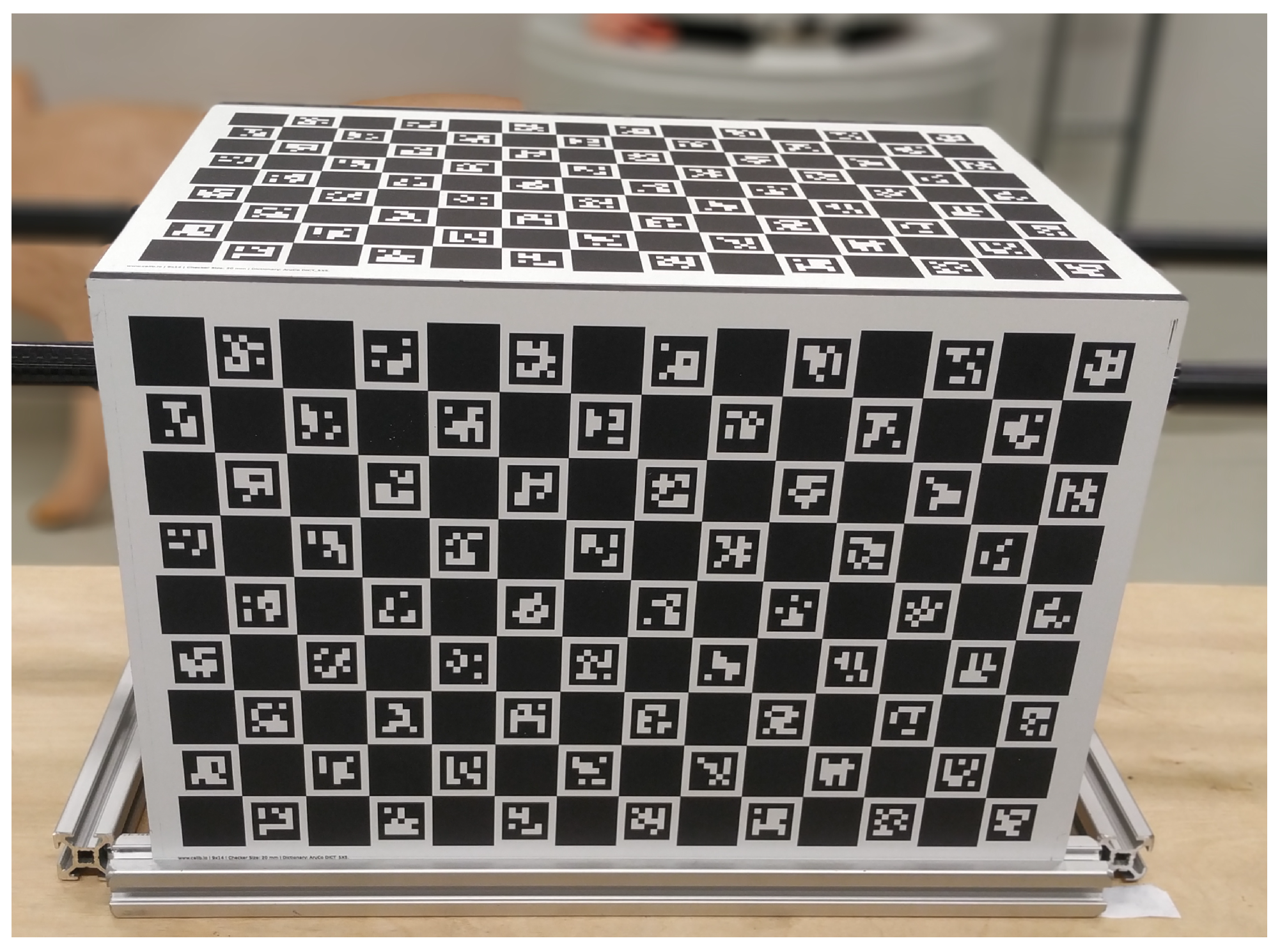
2.3. Methodology

The methodology used to measure the reconstruction error was based on a charuco cuboid with 3 faces, which was used to identify the points and calculate the RMSE. The chosen charuco boards were 300 mm by 200 mm, with a checker size of 20 mm and a marker size of 15.56 mm with 14 columns and 9 rows. This was manufactured using precision technology in aluminium by Calib.io (https://calib.io, accessed on 13 January 2022).

A charuco rectangular cuboid was built, as shown in Figure 7, using three boards.

2.4. Pre-Processing RGB-D Data

The first step was to improve the data by minimising the noise and the artefacts in the point cloud. To perform this task, some post-processing was applied to the captured frames.

In this work, the chosen post-processing methods were: alignment of colour and depth frame, sharpening of the colour frame and temporal and spatial filters applied to the frameset. Although the alignment and sharpening were always applied, the results were tested with both temporal and spatial filters enabled and disabled.

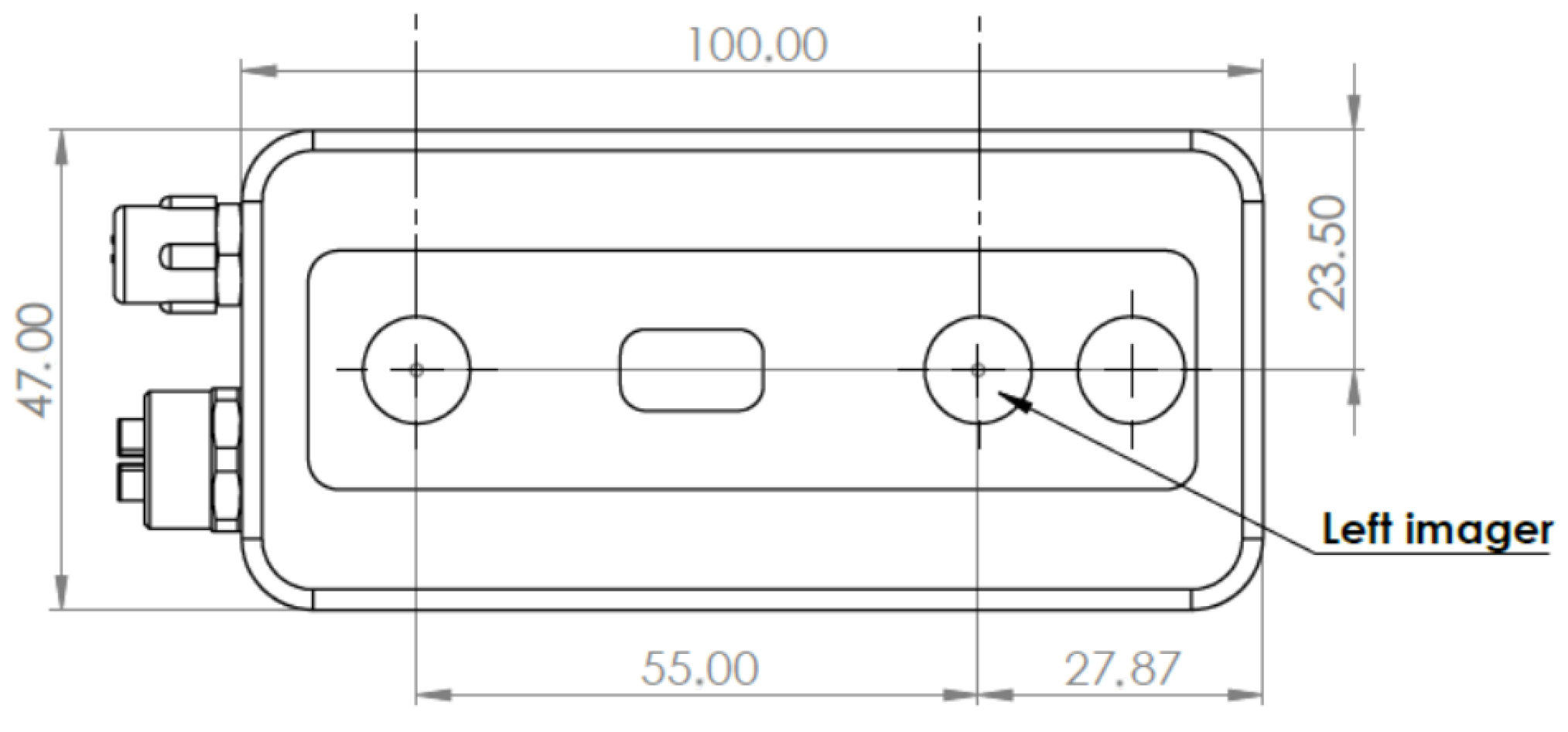
2.4.1. Alignment of Frames

The FRAMOS D415e camera had its origin reference in the left IR imager sensor and the RGB imager on the right side, as shown in Figure 8. As the sensors are different, an alignment between the colour image and the information was performed.

The alignment was performed in relation to the colour imager, i.e., the depth information was aligned to the colour frame. Since the alignment changes the relation of the pixels in the depth frame to match the colour sensor, the intrinsic matrix used to reproject the point cloud was also derived from the colour imager.

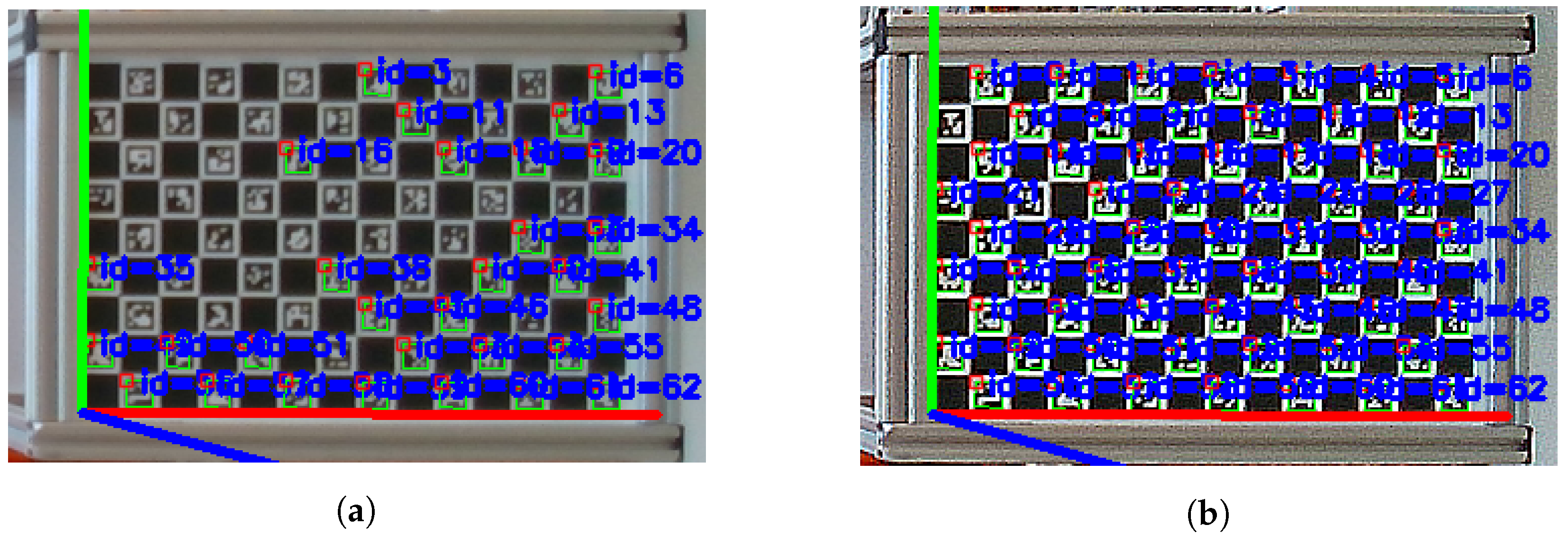
2.4.2. Sharpening Filter

Besides the alignment, a sharpening filter was applied to the colour image to improve the ArUco marker identification. The filter kernel used is shown in Equation (11).

$$\left|\begin{array}{ccc}-1& -1& -1\\ -1& 9& -1\\ -1& -1& -1\end{array}\right|$$

(11)

Figure 9a shows the charuco board before the sharpening filter was applied and the identified ArUco markers. Figure 9b shows the image after filtering, showing a significant improvement of the corners and edges. The sharpening filter improved the edges between the white and the black pixels of the board, increasing the number of identified ArUco markers.

2.4.3. Temporal and Spatial Filters

To diminish the noise artefacts of the data, two post-processing techniques were applied to the captured frames, a temporal filter and a spatial filter. Both filters were implemented in RealSense SDK and these have been well explained by Grunnet-Jepsen and Tong [39].

The temporal filter performs a time average of the frames to improve the depth calculation. The filter implements three parameters, those being the alpha, delta, and persistence filter. The alpha parameters represent the temporal history of the frames. The delta is a threshold to preserve edges, and the persistence filter tries to minimise holes by keeping the last known value for a pixel.

The spatial filter implemented in the SDK is based on the work of Gastal and Oliveira [40]. It preserves edges while smoothing the data. It takes four parameters, alpha and delta, which have the same function as in the temporal filter. This method also involves the filter magnitude, which defines the number of iterations, and hole filling parameters, which improve artefacts.

2.4.4. The Ground-Truth

After post-processing, the next step for the evaluation of the reconstruction is to generate a cuboid of reference points, in relation to the robot’s base, to be used as ground-truth data. This was performed based on the first camera data. The charuco board was identified and the markers’ corner was extracted from the image, as shown in Figure 6. Based on the cuboid geometry, the top reference was generated by rotating $-90°$ around the x-axis, followed by a rotation of 180° around the y-axis. Then, a translation of 280 mm, 187 mm and −190 mm in the x, y and z directions, respectively, was carried out, as shown in Equation (12). The backside was generated by rotating 180° around the y-axis and translating 280 mm and −200 mm in the x and z directions, respectively, as shown in Equation (13).

$${}_{top}{T}^b=T^0{\ast }_{cub}{T}^{cam0}\ast tran{s}_a\ast ro{t}_{x^{-90}}\ast ro{t}_{y^{180}}\ast {{(}_{cub}{T}^{cam0})}^{-1}$$

(12)

where ${}_{top}{T}^b$ is the transformation from the top of the charuco origin to the robot’s base, $T^0$ is the transformation from TCP to the base, ${}_{cub}{T}^{cam0}$ is the transformation from the first camera to the charuco, $tran{s}_a$ is the translation, $ro{t}_{x^{-90}}$ is the rotation in the x-axis, $ro{t}_{y^{180}}$ is the rotation in the y-axis, and ${{(}_{cub}{T}^{cam0})}^{-1}$ is the inverse transformation from the first camera to the charuco.

$${}_r{T}^b=T^0{\ast }_{cub}{T}^{cam0}\ast tran{s}_b\ast ro{t}_{y^{180}}\ast {{(}_{cub}{T}^{cam0})}^{-1}$$

(13)

where ${}_{top}{T}^b$ is the transformation from the top of the charuco origin to the robot’s base, and the other terms have been explained in the previous paragraph.

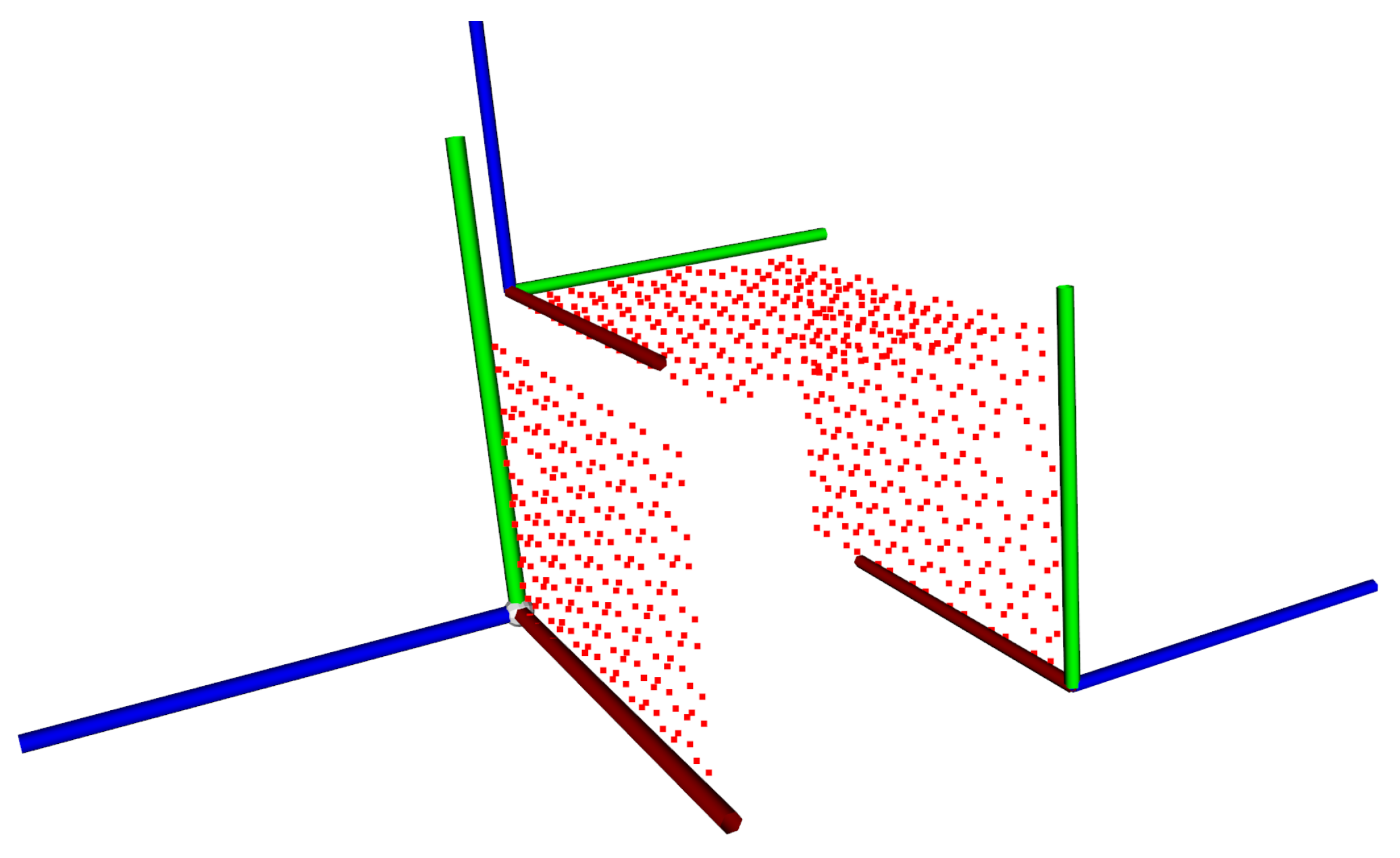
The final reference cuboid can be seen in Figure 10 with the coordinate system of every side shown as a visual aid.

The camera positions make it impossible to see only one charuco board at a time. To solve this challenge, the board can be rotated when it can be seen in at least two camera positions, or two (or more) boards can be used with known geometries.

In this work, two reconstructions were performed using the charuco board and one using a robotic arm’s position.

2.5. Charuco Cuboid

When using the charuco cuboid, each side is seen in two camera positions. Consequently, the pose estimation is based on the visible board. The defined origin for the reconstruction was set to be the first camera position. To obtain an optimal reconstruction, one must perform a rotation and translation on the data from camera positions, where the camera is facing a different board, based on the cuboid geometry, as explained in Section 2.4.4.

Notably, to calibrate all camera views (i.e., in all six possible positions), the charuco cuboid can remain stationary within the environment (i.e., it does not require repositioning for each camera).

2.6. Charuco Double-Sided Angled Board

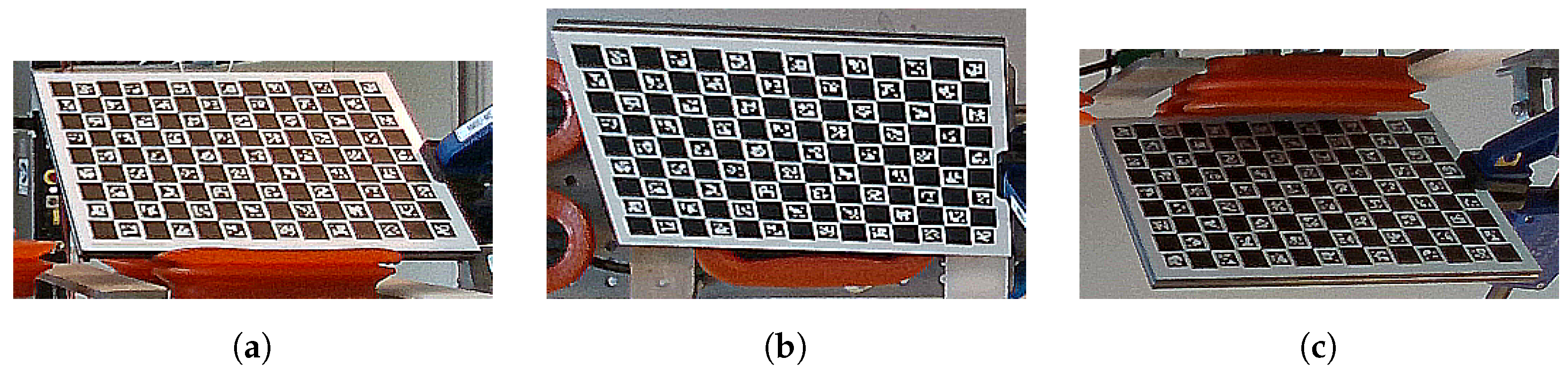
Using a double-sided board follows the same principle as the cuboid but is more simple since the camera can see the same side in 4 positions, and the back of the board in the other two, as shown in Figure 11a–c.

To perform the transformation, the left and the upper cameras were transformed to the inverse matrix of charuco to camera transformation (${}_{cha}{T}^{cam}$), to make the charuco board origin the same for these cameras. Then, the right cameras had to perform a 180° rotation around the y-axis and a translation of 280 mm and 1.2 mm in the x and z directions, respectively, according to the board geometry.

2.7. Robot’s TCP Transformation

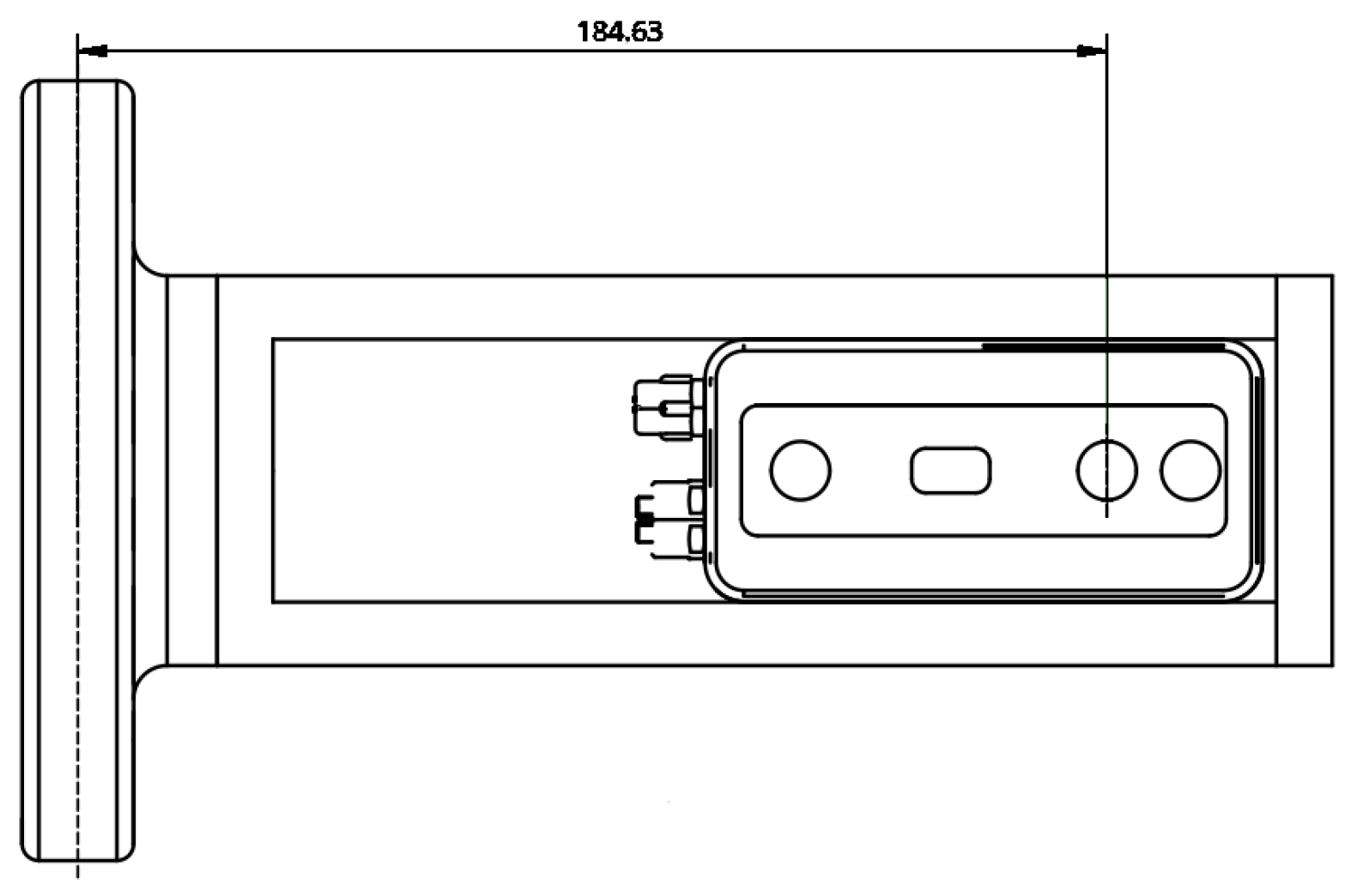
The robotic arm used in the setup was an ABB IRB 4600 40/2.55. The TCP position for every robot target position of the arm was recorded with the $x,y,z$ position and the rotation $q1,q2,q3,q4$ in quaternions. A transformation from the camera’s origin to the TCP was applied.

This transformation was calculated using the hand-eye calibration method proposed by Horaud and Dornaike [41]. A set of 30 different positions were defined for the calibration. The result was compared with the holder geometry, as seen in Figure 12.

The transformation found during calibration was the translation of $-0.050$ mm in the x direction, $-0.0442$ in the y direction, and $0.0780$ in the z direction, and rotations of $90.9179°$ around the x-axis, $1.1774°$ around the y-axis, and $0.4859°$ around the z-axis.

Pair Matching

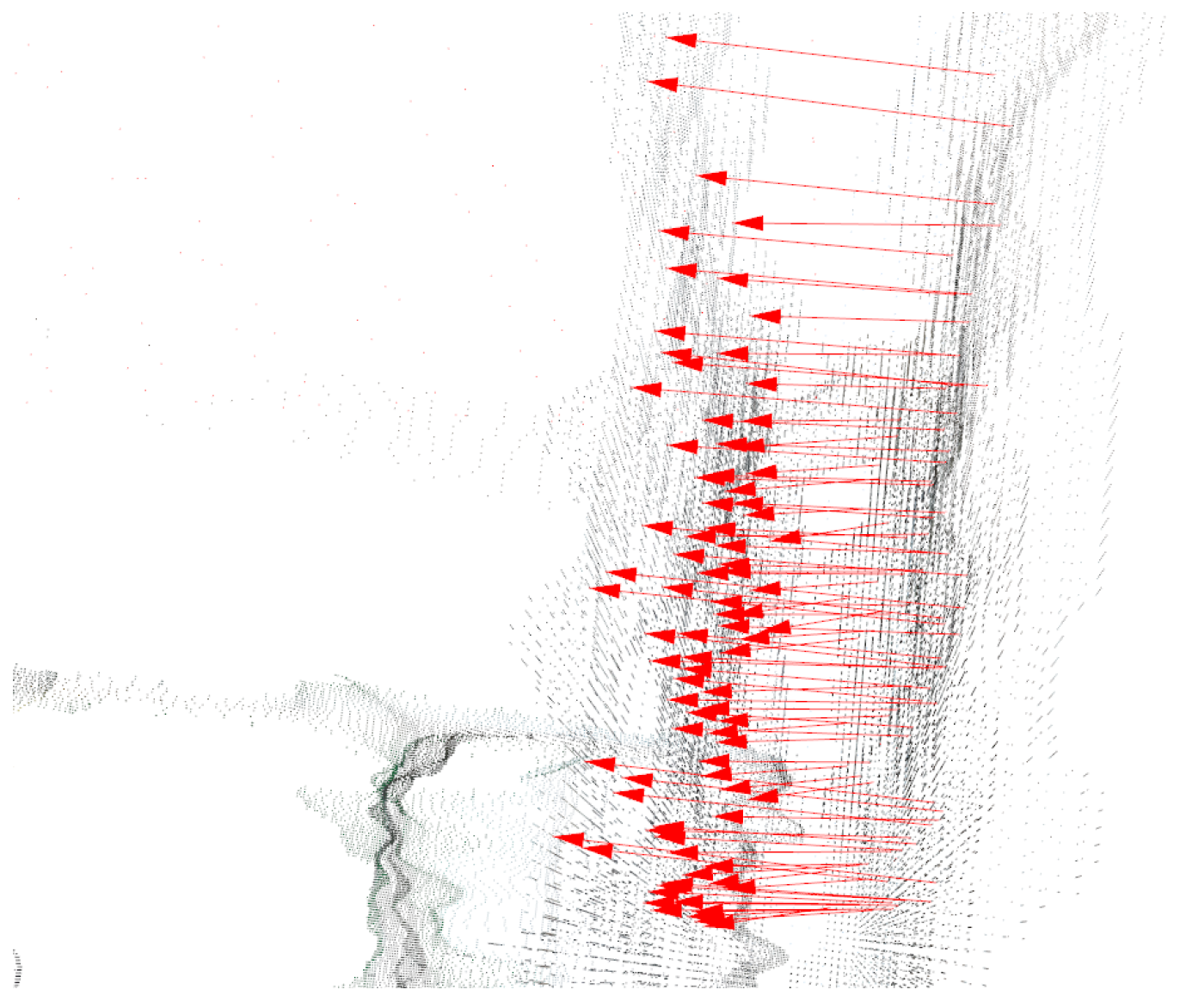
With the reference points ready, the transformation for each camera pose was solved based on the chosen methods explained above. The correspondent marker points were identified, and the metrics were calculated according to the explanation given in Section 2.1. Figure 13 shows arrows between the reference point and the board points, showing the correct identification of the pairs in which the error was calculated.

3. Results

The results of the reconstruction follow the metrics explained in Section 2.1. The first step was to identify the two most accurate methods for the 3D reconstruction of the scene. For this, each system used 1188 points to calculate the reconstruction error for the six camera views.

Table 1. Summary results with MAE, MSE, and RMSE for one set of data.

Method	MAE	MSE	RMSE
Charuco cuboid	7.5812	5.7475 × 10${}^{-2}$	6.8093
Double-sided Angled	10.12	0.1156	10.75
Robotic Arm	3.9888	1.5886 × 10${}^{-2}$	3.7121

shows the mean absolute error (MAE), the mean square error (MSE), and the root-mean-square error (RMSE) of each system, expressed in millimetres. It is interesting to note that the MAE and the RMSE exhibit a large difference, meaning that there was not a high discrepancy between the errors.

Based on these results, a program was written to run 20 sets of data for each method, with each set calculating the error between approximately 1188 points, depending on how many markers were found by the charuco algorithm.

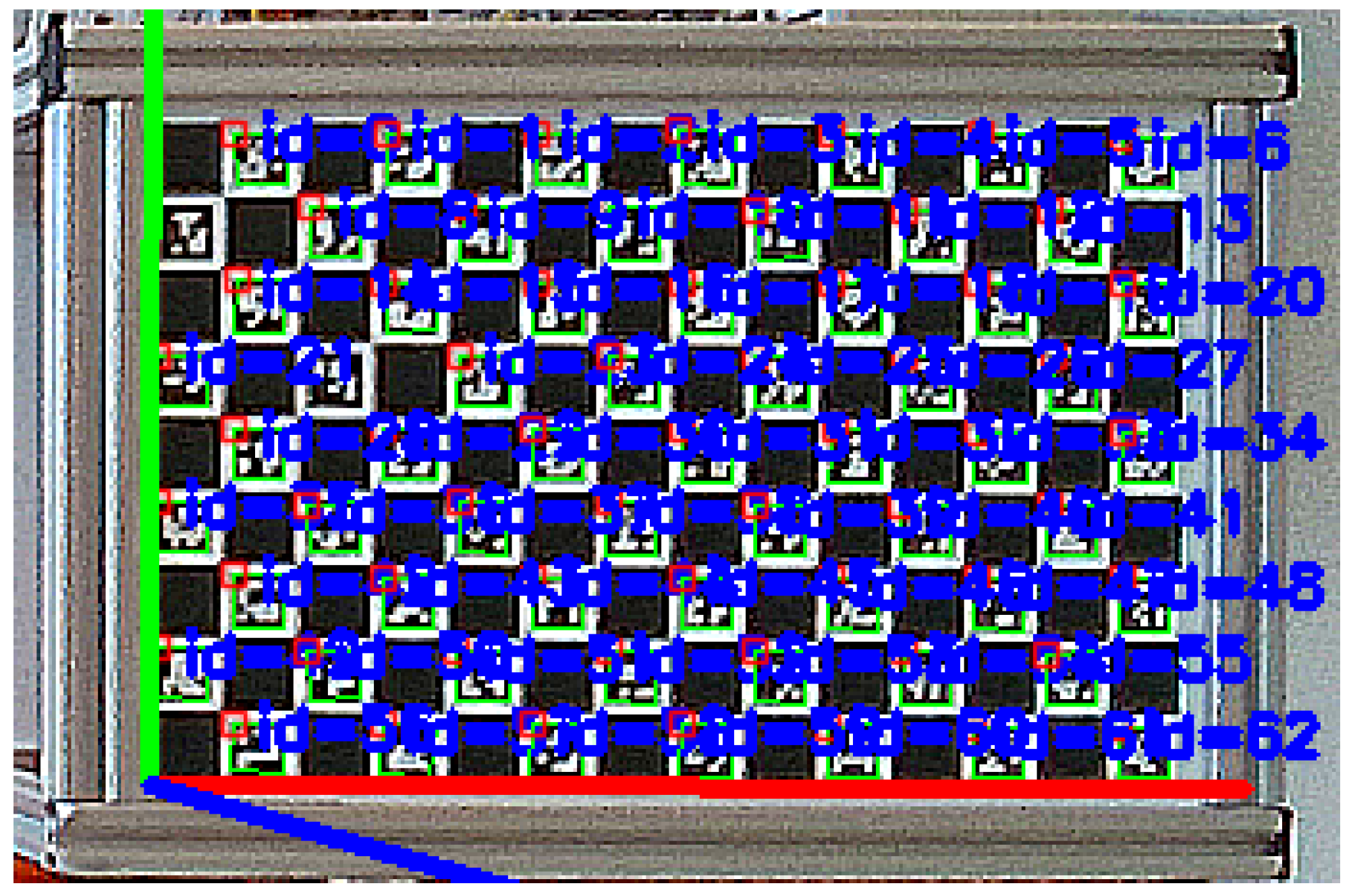
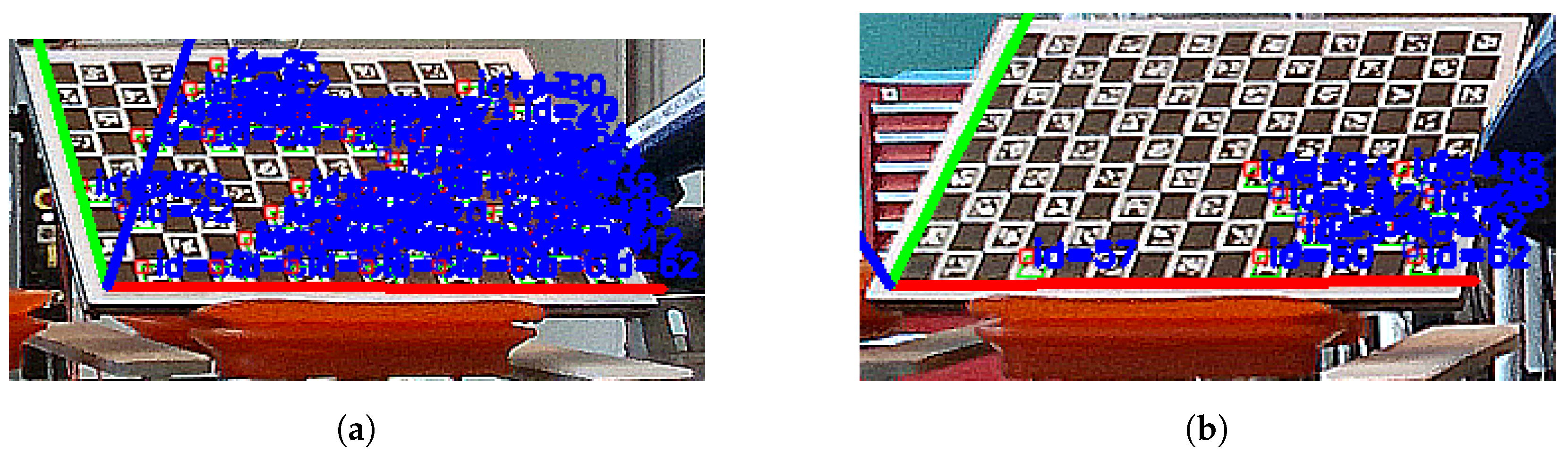
3.1. Charuco Double-Sided Angled Board

The double-sided board with an angle (to enable four cameras to see it simultaneously) exhibited a poorer performance when compared with the other two methods. The angle applied to the board made it harder to identify the markers, as shown in Figure 14a,b, possibly making it less accurate than the other methods.

Visually, it was able to calculate the pose well in the 2D image, but there was a degradation in the RMSE, which in this case was 10.12 mm.

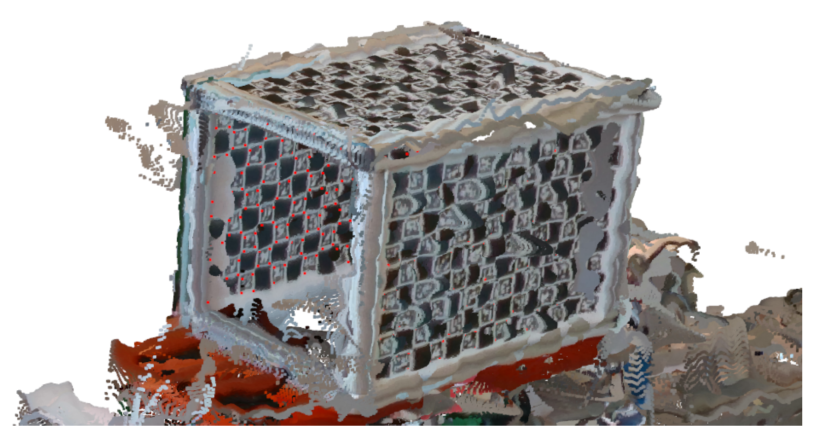
Figure 15 shows a detail of the reconstructed image with the double-sided charuco board, where small gaps between the top and lateral panel can be observed.

Due to this method’s less accurate 3D reconstruction compared to the other methods, we focused more on the other methods discussed below.

3.2. Cuboid vs. TCP Reconstruction Accuracy

The program was written in C++ using the Qt Library (https://www.qt.io, accessed on 8 February 2022), and it is available at GitHub (Please see “Data Availability Statement”), together with the dataset captured.

The program iterated over a directory with the files and calculated the RMSE, the mean squared error (MSE), and the mean absolute error (MAE) for both chosen methods. In addition, it assisted with the visualization of the point cloud.

The program was executed with both filtered and unfiltered data, as explained in Section 2.4.

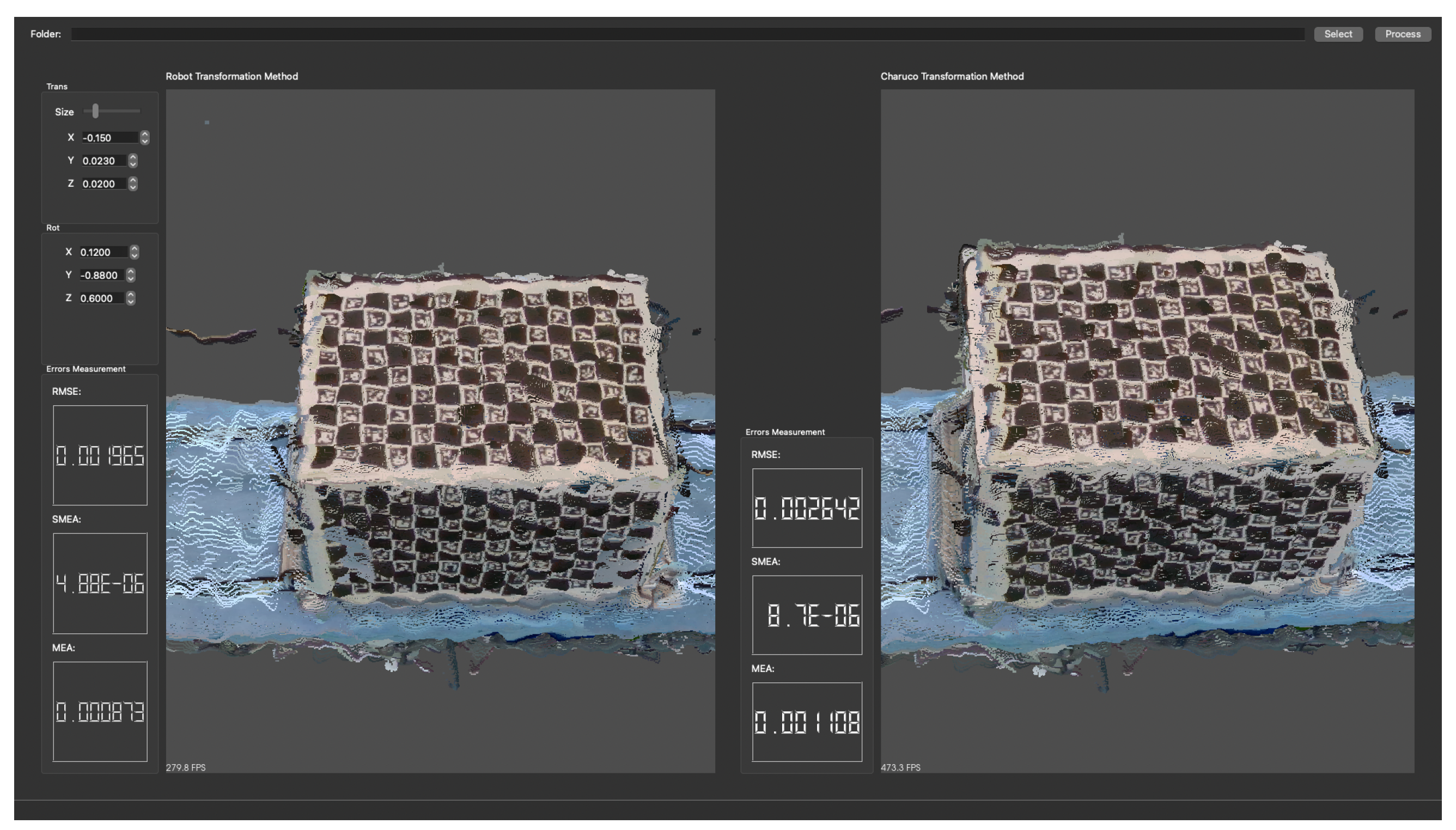
3.2.1. Unfiltered Data

After running the program for the 20 sets, a total of 23,117 paired points were used to calculate the error values. Figure 16 shows a screenshot of the program after the calculation with the reconstruction of the point cloud for both methods, with the TCP method on the left and the cuboid on the right side.

Table 2. Summary results for cuboid and TCP reconstruction with MAE, MSE, and RMSE for unfiltered data.

Method	MAE	MSE	RMSE
Charuco cuboid	1.10809	8.6994 × 10${}^{-3}$	2.6417
Robotic Arm	0.8734	4.8808 × 10${}^{-3}$	1.9651

summarises the results, showing a smaller error for the TCP method.

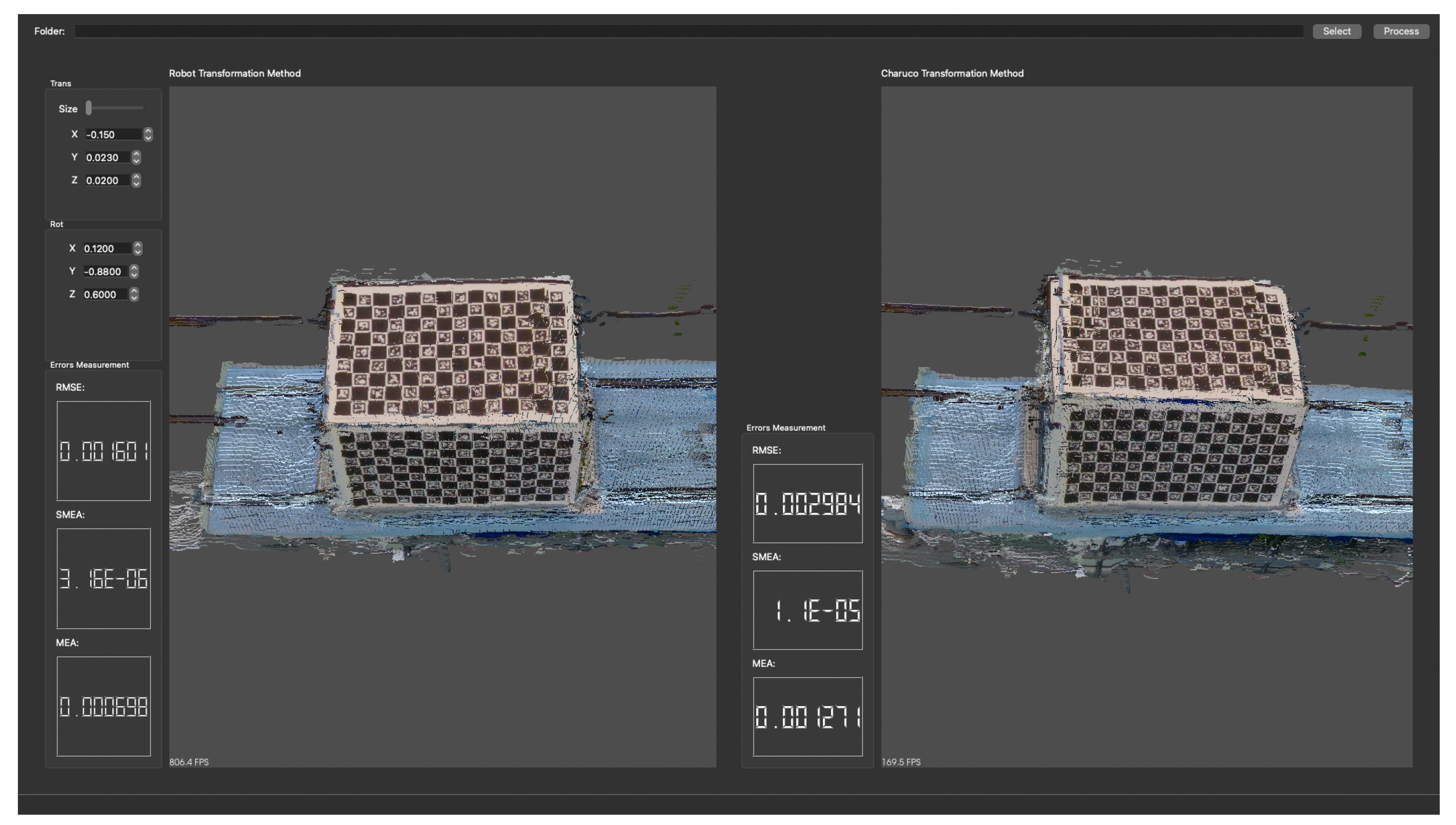
3.2.2. Filtered Data

For the filtered data, a total of 23,603 paired points were used to calculate the error values. Figure 17 shows a screenshot of the program after the calculation.

Table 3. Summary results for cuboid and TCP reconstruction with MAE, MSE, and RMSE for filtered data.

Method	MAE	MSE	RMSE
Charuco cuboid	1.2708	1.0987 × 10${}^{-2}$	2.9837
Robotic Arm	0.6983	3.1597 × 10${}^{-3}$	1.7432

summarises the results obtained, again showing a smaller error for the TCP method.

3.3. Charuco Cuboid

The reconstruction using the charuco cuboid had a low RMSE of 2.9837 mm for the filtered set, and an RMSE of 2.6417 mm for the unfiltered set, showing a better result for the unfiltered dataset.

3.4. Robot’s TCP Transformation

The robotic arm ABB IRB 4600 had a payload of 40 kg and a reach of 2.55 m. It had a position repeatability of 0.06 mm, a path repeatability of 0.28 mm, and an accuracy of 1 mm [15]. With this precision, the reconstruction showed the best performance with an RMSE of 1.7432 mm for the filtered dataset and an RMSE of 1.9651 mm for the unfiltered. In this method, the filtered dataset showed an improved result in relation to the unfiltered dataset.

4. Discussion

The accuracy of the reconstruction is vital to robotics tasks when using depth information to generate trajectories for a robot in a large scene. The usage of depth stream to reconstruct the scene, as in Newcombe et al. [42], may not be appropriate if the system is time-sensitive. It is faster to move the robotic arm to positions at a high speed and then capture a frame than it is to cycle through at a slower speed to capture the data.

The algorithms currently available for point cloud registration, such as iterative closest point (ICP) [16,43] and its variants, as well as other methods that try to find the transformation between point clouds, use overlapping, which in this case is minimal due to the fact that the observed scene is large. Moreover, they are too slow to be used in a time-sensitive system.

The ABB IRB 4600 has a preset maximum speed of 7000 mm/s, and the axis speed varies from 175°/s (axis 1) to 500°/s (axis 6). With these high speeds, the data acquisition and reconstruction can be sped up through a straightforward mathematical approach, such as the TCP transformation method. The idea is to have a fast and reliable transformation for the camera positions.

Further investigations could involve the study of how the trajectory generated for the TCP is affected by the errors in the reconstructions. Understanding this impact could help in developing a faster method without having repercussions on the desired output.

This work will assist in developing new designs and understanding one’s options when responding to reconstruction challenges using multi-camera views and a robotic arm. It casts light on two different approaches and how to evaluate the reconstruction of the 3D scene. However, it is not an exhaustive study on the topic.

5. Conclusions

In this study, we evaluated three pose estimation methods for RGB-D (3D) cameras in the context of 3D point cloud reconstruction. We proposed a method to identify the point pairs, and performed error measurements. Using a charuco cuboid, we identified and labeled the corner of the ArUco markers in order to create a pairwise set of points to measure the error values.

Two of our developed methods used the charuco board to estimate the pose of the cameras, whereas the third method used the robots’ TCP position to calculate and transform the point clouds to reconstruct the scene. The data were captured with a fixed position and at a distance of around 1 m from the board in each direction.

This distance reduces the resolution of the charuco board and consequently reduces the camera’s ability to recognise markers on it. To improve the recognition of markers, a sharpening filter was applied. Further filters were used to mitigate artefacts in the point cloud, due to the stereo vision system used by the camera.

Two methods, the cuboid and TCP methods, provided a good reconstruction with low RMSE values, taking into account the often noisy nature of point clouds derived from RGB-D cameras. The double-sided angled board had the highest RMSE, and it was excluded from further assessments. The increased error was assumed to be a result of the combination of the angle and distance from the camera. The robot’s TCP position had a high accuracy, exhibiting the best overall performance.