Article

Quality Assessment of Components of Wheat Seed Using Different Classifications Models

by
Zargham Fazel-Niari
1,*,
Amir H. Afkari-Sayyah
1,
Yousef Abbaspour-Gilandeh
1,
Israel Herrera-Miranda
2,
José Luis Hernández-Hernández
3,4 and
Mario Hernández-Hernández
3,4,*
1
Department of Biosystems Engineering, College of Agriculture and Natural Resources, University of Mohaghegh Ardabili, Ardabil 56199-11367, Iran
2
Government and Public Management Faculty, Autonomous University of Guerrero, Chilpancingo 39087, Guerrero, Mexico
3
National Technological of México/Campus Chilpancingo, Chilpancingo 39070, Guerrero, Mexico
4
Faculty of Engineering, Autonomous University of Guerrero, Chilpancingo 39087, Guerrero, Mexico
*
Authors to whom correspondence should be addressed.
Appl. Sci. 2022, 12(9), 4133; https://doi.org/10.3390/app12094133
Submission received: 18 March 2022 / Revised: 12 April 2022 / Accepted: 12 April 2022 / Published: 20 April 2022
(This article belongs to the Section Agricultural Science and Technology)

Abstract

:
To use machine vision technology in visual quality control of cereal seeds, sufficient knowledge is necessary. In this work, the capability of machine visual systems, equipped with industrial digital cameras for the identification and classification of seven-grain groups in wheat seed samples, was studied. Two statistical models and three support vector machines were employed in this study. Through image processing of 21,000 single grains, the shape, colour, and textural features of each grain were determined. Ninety-one features were ranked through the ReliefF method. The shape features were the most prominent, followed by the textural and colour features. Among the five models tested, the highest classification accuracy was obtained using quadratic support vector machine (QSVM) and the first 35 features. In the test run of this model with independent data, the classification accuracy for sound white wheat, small white wheat, broken white wheat, shrunken white wheat, red wheat, barley and rye were, respectively, 98.7, 98, 99.3, 90.7, 99, 100, and 97.3%, with an overall average accuracy of 97.6%. In the context of this study, the machine vision system—comprising an industrial digital camera and quadratic support vector machine or non-linear discriminate analysis method—was identified as a valuable system in the investigation of the visual qualities of wheat seeds.

1. Introduction

Seed quality determines the production rate, price, and quality of the final agricultural product. To produce high-quality wheat grains without any alien kernel, a strict evaluation of wheat seeds is necessary before packaging. Currently, the main portion of the wheat seeds is processed in cereal winnowing factories. Quality control experts take samples from the seeds produced after winnowing and the seed is manually certified along with the plant in seed laboratories of different research centres in the provinces. A decision for grading wheat is limited to the study of the visual qualities of seed samples by trained individuals. Manual operations affect the evaluated results in accordance with the personal experiences of the investigator. Different operational contexts, personal judgements, and fatigue levels influence the results of quality decisions by inspectors and experts. Human mistakes and mood fluctuations cause problems in quality control assessments of wheat seeds. It is a difficult, time-consuming task, calling for experienced staff. In Iran, wheat breeding researchers frequently encounter such problems while measuring and comparing the visual qualities of wheat seeds manually. During winnowing, it is necessary to check the output product to assess the operations of the cleaning unit.
Thus, quantitative and objective methods for measuring cereal features are useful and will be required in the future. Machine vision systems have been widely used in different research areas and recent technological developments in computer sciences and image processing have expanded the use of digital images. Recent studies have indicated that image processing is one of the key elements in developing automatic evaluation systems for crops. The results indicated that the digital image processing system is much more accurate in comparison with the manual methods [1]. By employing this advanced tool, one can attain standardization, integration, cost reduction, and improvement in quality control while increasing accuracy and reducing time. Regarding the classification of cereals and the alien grains, extensive studies have been conducted worldwide, and a limited number of them were conducted in Iran. To present a machine vision system for quality control of wheat seeds, it is required to conduct thorough and foundational research.
These studies have identified and classified wheat and barley grains variety through image processing with an acceptable accuracy [2,3,4,5,6]. For a single-seed classification of red wheat, durum wheat, barley, wild oat, and rye, using three groups of features (shape, colour, and texture), a thorough study was conducted with a video camera [7]. The highest accuracy in this research belonged to the model comprising three group features: shape, colour, and texture. To identify damaged wheat grains, the images of grains while falling were captured by a high-speed digital camera and subsequently processed. By using LDA (linear discriminate analysis) and KNN (K-nearest neighbour) methods, an accuracy of 91–94% was obtained [8]. Some researchers reported that not only the cereal grains but also the dockage in samples can be accurately classified by machine vision systems [9].Colour and texture features are more helpful in combination than alone in grain classification [10]. One can attain the highest accuracy in classifying wheat and barley by considering three features: maximum radius, green band mean, and grey-level co-occurrence matrix (GLCM) at 90° [11]. Visual features of wheat based on digital image processing work very well in identifying the germinated and musty wheat seeds [12].
A literature review shows that, in normal imaging, machine vision technology uses grain feature differences such as shape, texture, and colour for the identification of product verity and constituent elements. In past studies, different sizes of a wheat grain and attributes of being shrunken or broken in conjunction with other grains have not been studied simultaneously. In the classification, there are either two groups of sound and impaired wheat seeds, or several groups of sound seeds. In addition, past studies have used a digital camera, a video camera, or a scanner. To date, there are no reports of using an industrial digital camera to classify cereals. The study of the production process of certified wheat seeds has been the basis for selecting grain groups in this study. Barley grains, rye, and foreign wheat cultivars are difficult to distinguish in the field due to their similarities in appearance and the physical characteristics of these grains to the main seed wheat passing through threshing machines and reaching the bagging stage. This includes broken, small, and wrinkled grains. The main purpose of this study is to employ a machine vision system based on an industrial digital camera for the classification of seven groups of qualified wheat seed and foreign grains including sound white wheat, small white wheat, broken white wheat, shrunken white wheat, red wheat, barley, and rye. The ranking of features, application of support vector machine classification technique, and classical methods of statistical discrimination are also examined.

2. Materials and Methods

The general process of the machine vision system constitutes a hardware section for preparing the images and subsequently transferring them to a software section. The software deciphered the features of kernels and modelled them for classification. The workflow included preparation of samples, image capture, image processing, deciphering, feature ranking, modelling, and finally comparison of the classifiers.

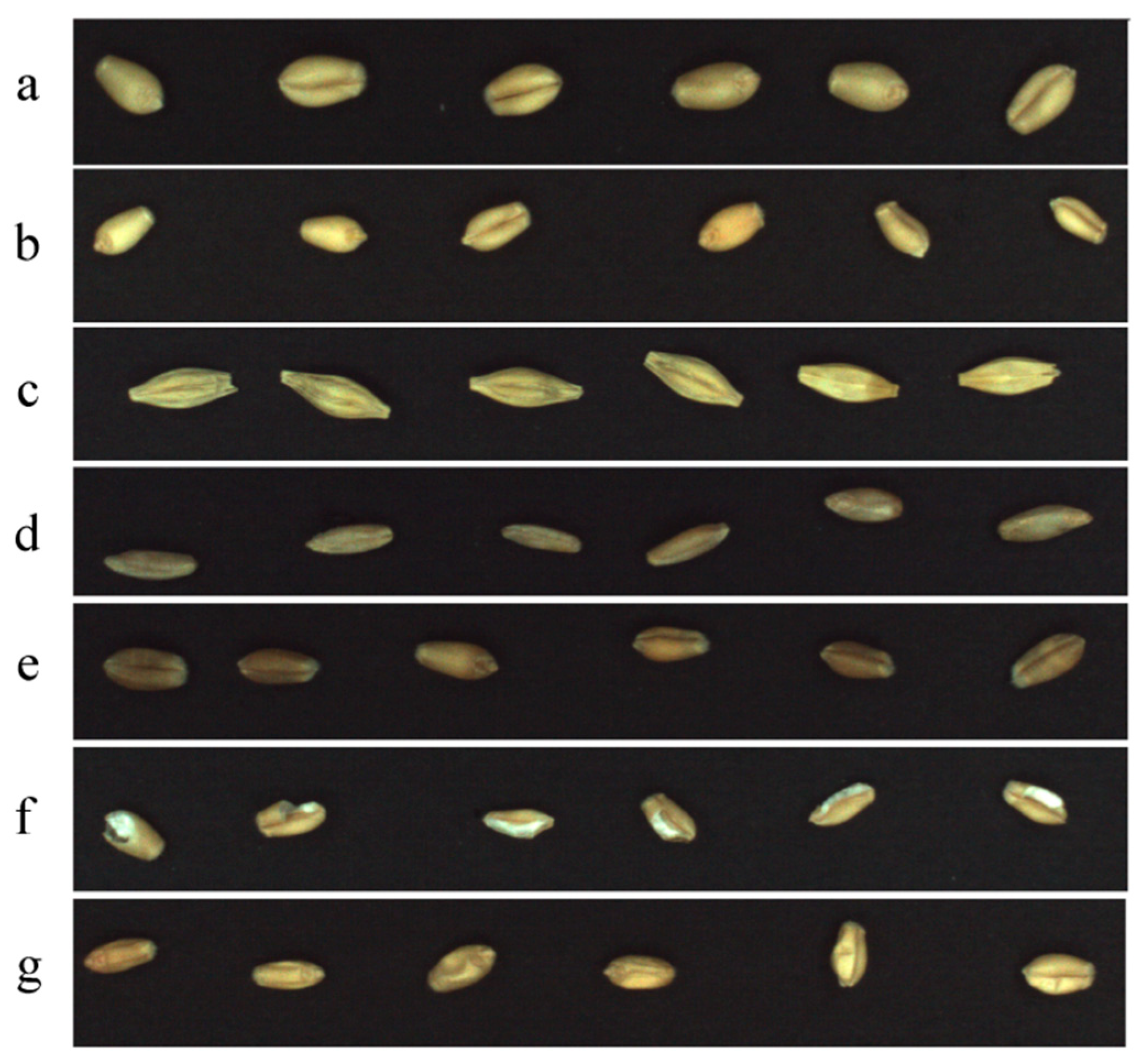
2.1. Preparing Grain Samples
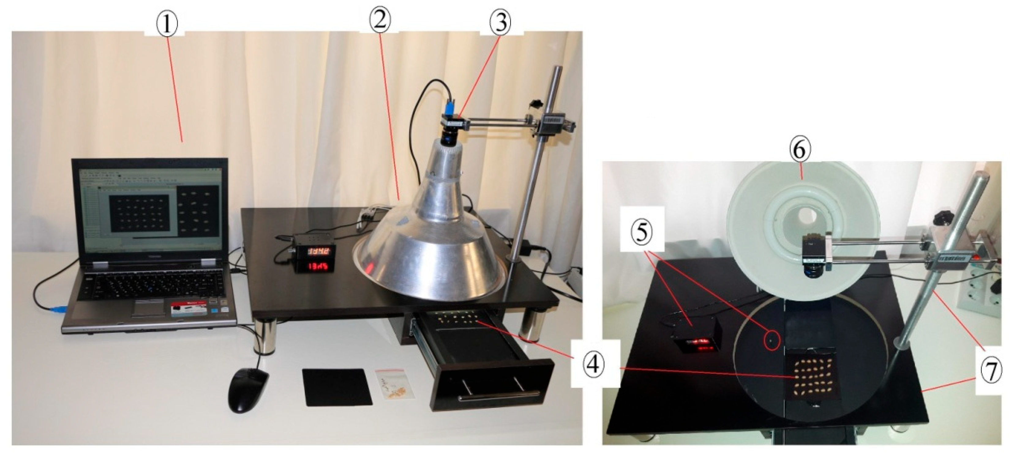
The Morvarid wheat variety was selected as the basic seed for white wheat and four-grain groups, including sound white wheat, small white wheat, broken white wheat, and shrunken white wheat, which were prepared from it. The other three groups were the grains of red wheat (Zagros variety), barley, and rye. The barley samples were prepared by mixing four local prevalent barley varieties (Bahman, Dasht, Khorram, and Makuyi). The seven-grain groups were gathered from four seed-processing factories in different regions of Ardabil province. From each constituent group, 100 samples were selected, each containing 3000 grains of each variety; separated; and packaged. An image of the grain groups is presented in Figure 1.

2.2. Imaging

An industrial digital camera (DFK72AUC02) with a CMOS sensor type was used for imaging. Unlike the prevalent cameras and camcorders, the horizontal and vertical pixels in this camera are equal, a value of 2.2 µm, with horizontal and vertical resolutions of 2592 and 1944, respectively. To prevent image distortion in imaging margins, a Japanese telecentric lens (MP1614_mp2, focal length 16 mm, Type 2/3 model, Coputar Company) was attached. The camera was installed at a distance of 30 cm from the panel on which seeds were placed. Local calibration of the camera was performed using three coins with a specific area. The relationship between the number of pixels and measurements of the real sample was determined. Circular daylight fluorescent lamp [13] with a power of 22 watts and a conical chamber were used for lighting. To standardize the light conditions, the inner wall of the lighting chamber was painted white and then coated with magnesium oxide [14]. Between the lens of the camera and the circular lamp, a metal wall was placed to receive the reflected light from the grain samples. A photo resistor sensor controlled the stability of the light intensity. The camera was connected to a portable computer via a USB cable (shown in Figure 2). Owing to the high applicability and functionality of MATLAB, all ofthe programs and algorithms of the camera connection, image processing, modelling, and evaluation of classifying methods were analysed by MATLAB version 2015a. The programs were run in Toshiba TECRA_A9 series portable computer. The computer was equipped with an Intel dual core processor of 2.20 GHZ (Intel-R Core TM 2 Duo CPU), 1 GB RAM, and Windows XP sp3 operating system.
A black Steinbach cardboard (code 08) was used as the panel on which the grains were to be placed. Cardboard stencils were prepared with 30 holes of exactly the size of wheat grains. After putting each sample with 30 grains on the stencil over the black panel, the stencil was removed. The separated grains were put in the rail drawer, and by moving the drawer inside the lighting chamber, the grains were exposed to the camera’s field of view. By running the graphical user interface program, the image of the sample was observed on the monitor, and by pressing the record button, the image of the grain was saved in the computer in RGB mode and five-megapixel resolution. In this way, 700 images (100 images of each grain variety) were obtained. Each image was composed of 30 grains.

2.3. Image Processing

An integrated program was written to conduct the pre-process operations and to decipher shape features and, by calling the functions of texture and colour features (separately written), to calculate and save the collection of features for each grain. Algorithm implantation was as follows: (1) importing the image, (2) cropping the image to the dimensions of 2590 pixels length and 1990 pixels width, (3) conversion to greyscale, (4) binary thresholding of pixels against background, (5) conversion to the binary image, (6) filling the probable inner empty space of the grains, (7) noise removal, (8) grain labelling, (9) calculation of the shape features, (10) multiplication of obtained binary images the in the labelling phase by the three-coloured layers of the original image and generating the noiseless colour image, (11) rotation of the images of the grains to the horizontal axis, (12) calling the colour computation function, (13) calling the texture computation function, and finally (14) saving all of the features based on the class of each grain in a table. After imaging with accurate and controlled lighting, the most important step in pre-processing was the determination of the threshold value for conversion of the grey image to the binary. The threshold must be implemented in such a way that the edge borders of grain varieties are completely separated from the background. The result of this section influences all of the calculations and, subsequently, the classifications. Three methods were used to determine automatic threshold: Otsu threshold [15]; the proposed algorithm by Guevara; and the image histogram threshold of Parker, which uses repetitive processes [11]. These three methods were used for both individual groups and their combinations. Considering the results obtained and the histogram of the images, the optimized threshold value of 0.25 was applied in the processing of all images. That way, there was no need to calculate the value of threshold for each image separately.

2.4. Calculating the Shape Features

The algorithm for morphological features was written in the main image pre-processing program, which upon receiving the binary and labelled image, calculated the features separately for each grain. By using the calibration coefficient, the length unit was converted from pixels to millimetres and the features were converted accordingly. Calculations of the features such as area (A), periphery (P), main axis length, smallest axis length, length, width, rigidity, equivalent diameter and eccentricity was conducted by the regionprops function in MATLAB tools. For calculating other features, the following functions were employed in MATLAB:
Thinness Ratio (TR): It measured the roundness of the kernel.
TR = P 2 4 π A
Aspect Ratio: Major Axis Length/Minor Axis Length.
Rectangular Aspect Ratio: Length/Width.
Area Ratio: (Length × Width)/Area.
Maximum Radius (mm): It was the maximum distance between a pixel on the boundary and the centre of the kernel.
Minimum Radius (mm): It was the minimum distance between a pixel on the boundary and the centre of the kernel.
Radius Ratio: Maximum Radius/Minimum Radius.
Mean Radius ( µ R ): It was the mean of all radii of the kernel region.
Standard Deviation of all Radii ( σ R ): It was the standard deviation of the distances of all pixels on the boundary from the centre of the kernel.
Haralick Ratio: µ R / σ R .
Fourier Descriptors: The one-dimensional distance function d k was calculated for all pixels on the boundary of a kernel as follows:
d k = [ ( i k c ik ) 2 + ( j k c jk ) 2 ] 1 / 2
where
( i k , j k ) = kth pixel coordinates on the boundary of the kernel;
( c ik , c jk ) = centroid of the kth kernel.
The magnitude of the Fourier descriptors was calculated as follows:
FD u = [ R u 2 + I u 2 ] 1 / 2
For u = 0, 1, 2, … (N − 1). The real value of the descriptor was defined as follows:
R u = k = 0 N 1 d k · cos [ 2 π ku N ]
Additionally, the imaginary value of the descriptor was defined as follows:
I u = k = 0 N 1 d k · sin [ 2 π ku N ]
where
N = number of pixels on the boundary of the kernel.
The first seven Fourier descriptors (u = 0, 1, 2, 3, 4, 5 and 6) were used for analysis.
Calculating moments: Spatial moments are a set of invariant moments, insensitive to transition, congruence, reflection, and rotation [11]. These moments are statistical measurements of the object’s attributes. Seven standard invariant moments were calculated for the binary image of each grain using normalized central moments introduced by [15]. A total of 31 shape features was found for each grain.

2.5. Calculating Colour Features

The function defined for deciphering colour features received the colour image and, after isolating three colours of red (R), green (G), and blue (B), started the calculations as follows:
First, the values of HSI were calculated by the following equations [15].
I = R + G + B 3
S = 1 3 Min ( R , G , B ) I
H = cos 1 { 1 2 [ ( R G ) + ( R B ) ] [ ( R G ) 2 + ( R B ) ( G B ) ] 1 2 }
where I is the colour intensity, S is saturation, and H is hue. The values of RGB were normalized by dividing with the value of R + G + B. The value of HSI was in the range from 0 to 1. Equation (8) generates the values of H at 0°–180°, 0 ≤ H ≤ 180. If (B/I) > (G/I), then H will be greater than 180°. In this situation, the value of H is calculated as (360 − H); then the value of H is divided by 180 to maintain a range of 0–1. When R = G = B, the value of S is zero, making it meaningless to define angle H, in which case H was also assumed to be 0. When R, G, and B were zero, then I = 0 and both H and S were undefined. In such situations, S and H were assumed to be 0 [16]. The number of pixels in each grain image (area of the grain) is considered the frequency of single colours. The 3 parameters of mean, variance, and standard deviation for six single colours (R, G, B, H, S, and I) were calculated, and finally, 18 colour features were extracted for each grain image.

2.6. Calculating Texture Features

The specific function for deciphering texture features receives the horizontal colour image in the four-square periphery of each grain and then calculates the texture features. The aforementioned algorithm extracts three primary colours of red, green, and blue (R, G, B) and their constituents {X = (R + G + B)/3}, {X1 = (3R + 2G + B)/6}, {X2 = (2R + 1G + 3B)/6} and {X3 = (1R + 3G + 2B)/6}. In this way, the special colour bands or the constituents in classification will be determined with better accuracy. To reduce calculation time, the grey level intensity of the images was reduced from 256 to eight in all mentioned seven bands. Then, the grey-level co-occurrence matrix (GLCM) was calculated independently. By dividing GLCM of each colour band by all the elements of the matrix, the normalized values were obtained. Six texture features were defined for each of the seven colour bands, i.e., a total of 42-texture features were defined for each grain. These were extracted as follows [15]:
Contrast = i = 1 K j = 1 K ( i j ) 2 p ij
Homogeneity = i = 1 K j = 1 K p ij 1 + | i j |
Correlation = i = 1 K j = 1 K ( i m r ) ( j m c ) p ij σ r σ c
Energy = i = 1 K j = 1 K ( p ij ) 2
Entropy = i = 1 K j = 1 K p ij log 2 p ij
Variance = σ r ×   σ c
where i and j are the rows and columns of the normalized co-occurrence matrix (pij); K is the intensity of grey level images (K = 8); and m c and m r , and σ r and σ c are, respectively, the means and standard deviations obtained by summing over the rows and columns of the normalized co-occurrence matrices.

2.7. Ranking Features

The application of more features than the optimum not only decreases the accuracy of classification but also impairs the classifying operation [9]. There are examples in which independent but noisy features provided poor statistical information. Among different methods for reducing features, the ReliefF algorithm works well for correlative and noisy features, and it can calculate the correlation between features and the related groups [17]. Generally, we should select features with less noise and significant different values in each group. To determine the importance of each feature and to select from 91 items, the ReliefF algorithm in MATLAB was employed to conduct the ranking operations. This algorithm first chooses a sample subset from the training samples collection. The user must define the number of samples in this subset and place it as the input of the algorithm. By trial and error, the suitable number of samples was determined to be 15. The algorithm chooses a sample from this subset in random; then, for each feature of this sample, it finds the nearest hit and the nearest miss based on the Euclidean metric. After determining the nearest hit and the nearest miss, it updates the weights of the features. The bigger this value, the better this feature works in separating samples of one class from others.

2.8. Preparing Classification Models

In most studies, statistical classifiers have acceptable accuracy in classifying different groups of grains [1,11,13,18]. By using independent variables, these models create discriminate functions and through these functions, the classification and identification of groups are implemented. Statistical classification algorithms with the application of linear and quadratic statistical discriminate analysis were created in MATLAB, and by using them, linear discriminate analysis (LDA) and quadratic discriminate analysis (QDA) were trained for all the ranked features.
Another method of modelling is the classifiers of support vector machine (SVM). SVM works based on the statistical theory of Vapnik [19]. Briefly put, SVM algorithm transcends the training data by a non-linear mapping, and in this new dimension, it searches for a hyperplane that separates the samples of one class from another. This is a new method that has recently found wider uses in classification than other traditional methods such as perceptron neural networks [20]. Reports of the application of this method for classifying cereal grains have indicated good results [21,22,23]. By selecting three kernel functions (linear, quadratic, and cubic polynomial), the three models linear support vector machine (LSVM), quadratic support vector machine (QSVM), and cubic support vector machine (CSVM) were created by a one-against-one coding [19]. These models were ranked by the tenth to the last feature and were trained by an increase in five features per step. The model of support vector machine was created by the Gaussian function, but because of its weak performance, it is not presented here. In the training and determination of the accuracy of all five models, the evaluation and training data division was conducted by the k-fold cross-validation method. In this technique, each sample of the main data is placed in the training collection equally as others and is selected only once for testing. By determining a value for k, the collection of data is divided into k number of equal parts. One part is set aside for testing and the other part (k − 1) is used for designing the model. This process takes place for all k parts of the collection. The accuracy of the model is determined by calculating the mean of these k repetitions. Because of the large amount of data, the value of k equalled five in this research.

3. Results

The first 40 features of the ranked 91 items are indicated in Table 1. The features are ranked in descending order in accordance with their share of weight in the classification model. The first 10 features are related to shape, among which the area ratio is the most effective. The reason for this effectiveness is the differences ingrains in the edge and the uniformity of shape features in almost all grain groups except broken wheat. Among the first 35 top features, there are 16 shape features, 8 colour features, and 11 texture features. The share of colour features is less than the shape and texture features (Table 1). The eleventh and fifteenth to eighteenth features are average variances in the colours, and the reason for this is the colour combination differences of grain. As the variance in colour features increased in grain groups, their share in the top features decreased. The texture difference of grain surfaces and their low correlation brought them a good share of the top features. Among the effective features related to texture, single-colour entropy and different colour combination had the greatest shares. The reason was the difference in the texture of the grains surface and the randomness of colour intensity of the pixels in relation to each other.
The five classification methods presented in the Materials and Methods section were modelled in accordance with the 91 ranked features. The average of accuracy of classifiers in relation to the number of ranked features is presented in Figure 3. When using the top 10 features for classification, the accuracy average was low and less than 85%. By increasing the number of top features to 20, the accuracy average augmented up to 90% (91 to 94%) for all models, and it remained stable up to 30 features. When the features were increased to 35, the accuracy improved to 97%. Then, in support vector machines, this value was stable; in LDA, it had an insignificant increase; and in QDA, it decreased (Figure 3). The average classification accuracy of training models based on the top 35 features for each method, including linear support vector machine (LSVM), quantized support vector machine (QSVM), cubic support vector machine (CSVM), linear discriminate analysis (LDA), and quadratic discriminate analysis (QDA), were 96.8, 97.2, 96.9, 94.7, and 96%, respectively.
To predict seven-grain classes based on independent data, only the models created with 35 top features were employed. The results of the five selected models after the application of independent data are shown in Table 2. The least classification accuracy for seven-grain classes was 95%, observed in the linear discriminate analysis. The highest accuracy—97.6%—was observed in quantized support vector machine. The results of classification with independent data were not significantly different from those with training data, proving the interoperability of the models in predicting the class of new data. The classification accuracy of shrunken grains was the lowest in all models, and it was the factor for diminishing the accuracy in all models. Barley grains were classified with the highest accuracy in all models. In four of the models, they were classified with 100% accuracy (Table 2). This is in line with the studies reporting the high distinguishability of barley grains from wheat [11].
The time required for training support vector machine models is much more than that for statistical classification models. However, there was no significant difference in the classifying speed of the created model in encountering independent data. Thus, by relying on the importance of training time in relation to classification accuracy, one can choose the suitable model. Here, the quantized support vector machine was selected as the best model because of its highest accuracy. The interference matrix of this model in identifying new grains is presented in Table 3. The grains of sound white wheat, sound white wheat, broken white wheat, red wheat, barley, and rye had acceptable classification accuracies.

4. Discussion and Conclusions

A continuous increase in the number of classification features reduces accuracy. This fact was observed in the QDA model. Except for the first 35 features, the other features were almost insignificant. Thus, by leaving the classification accuracy untouched, they can be removed and one can only use the top 35 features of Table 1 in classifying seven-grain groups (sound white wheat, sound white wheat, broken white wheat, shrunken white wheat, red wheat, barley, and rye). An acceptable classification accuracy and the low intrusion of sound white wheat and red wheat grains is a consequence of their differences in colour and texture. Being uniform in colour and texture, barley grains were classified with 100% accuracy, while shrunken white wheat grains were classified with 90.7% accuracy. The similarities in colour and shape of shrunken white wheat with other grains except barley decreases classification accuracy in general. For example, 13 grains out of 300 shrunken white wheat were wrongly classified as sound white wheat class. Venora et al. [1] reached 95% accuracy in classifying shrunken white wheat by analysing the image of the transmitted light through the bulk of single-layer. It should be noted that the number of classes in their study was fewer than in the present work. The average of classification accuracy of this research is also lower than the work of Majumdar S. and D. S. Jayas [7]. They studied only five groups of complete cereal grains and used a camcorder for imaging. For this reason, they may have attained a higher accuracy. However, in comparison with the study of Paliwal et al. [7], this work had a higher classification accuracy. Since they had 10 classification groups, the accuracy was quite low.
By taking note of the obtained acceptable accuracy, one can conclude that imaging with the resolution of five mega pixels (1920 × 2560) is enough to evaluate the visual features of wheat. The use of fluorescent lamps in a closed (controlled) environment may suffice as a lighting system due to the stability of light intensity. The application of all the features, however, might decrease the classification accuracy. The suitable area for classification accuracy with lower number of features indicates the applicability of the ReliefF method in ranking features; a comparison of different methods, especially genetics algorithms, is highly recommended. Statistical classification models and support vector machines gave an acceptable accuracy by employing only 35 features (16 shape features, 11 texture features, and 8 colour features). The lowest classification accuracy in identifying seven groups of grains with the use of independent data was observed in the linear discriminate analysis (LDA) model. The quadratic support vector machine (QSVM) was proven to be of better applicability in this study. Barley grains were identifiable with the highest accuracy due to their shape differences. It can be concluded that the industrial digital camera and support vector machine classification methods or statistical methods have enough potential for classifying quality elements of wheat seed. It is possible to increase the identifiable groups if system training with new groups was required.

Author Contributions

Conceptualization, Z.F.-N., A.H.A.-S. and Y.A.-G.; methodology, Z.F.-N., A.H.A.-S. and Y.A.-G.; software, Z.F.-N.; validation, A.H.A.-S., Y.A.-G. and J.L.H.-H.; formal analysis, Z.F.-N., A.H.A.-S. and Y.A.-G.; investigation, Z.F.-N., A.H.A.-S., Y.A.-G. and I.H.-M.; resources, Z.F.-N., A.H.A.-S. and M.H.-H.; data curation, Z.F.-N., A.H.A.-S. and Y.A.-G.; writing—original draft preparation, Z.F.-N., A.H.A.-S. and Y.A.-G.; writing—review and editing, J.L.H.-H., I.H.-M. and M.H.-H.; supervision, A.H.A.-S. and Y.A.-G.; project administration, A.H.A.-S.; funding acquisition, Y.A.-G., J.L.H.-H., I.H.-M. and M.H.-H. All authors have read and agreed to the published version of the manuscript.

Funding

This study was financially supported by University of Mohaghegh Ardabili.

Institutional Review Board Statement

Not applicable.

Informed Consent Statement

Not applicable.

Data Availability Statement

The data presented in this study are available on request from the corresponding author.

Conflicts of Interest

The authors declare no conflict of interest.

References

  1. Venora, G.; Grillo, O.; Saccone, R. Quality assessment of durum wheat storage centres in Sicily: Evaluation of vitreous, starchy and shrunken kernels using an image analysis system. J. Cereal Sci. 2009, 49, 429–440. [Google Scholar] [CrossRef]
  2. Dubey, B.P.P.; Bhagwat, S.G.G.; Shouche, S.P.P.; Sainis, J.K.K. Potential of Artificial Neural Networks in Varietal Identification using Morphometry of Wheat Grains. Biosyst. Eng. 2006, 95, 61–67. [Google Scholar] [CrossRef]
  3. Pazoki, A.; Pazoki, Z.; Sorkhilalehloo, B. Rain fed barley seed cultivars identification using neural network and different neurons number. World Appl. Sci. J. 2013, 22, 755–762. [Google Scholar] [CrossRef]
  4. Pourreza, A.; Pourreza, H.; Abbaspour-Fard, M.H.; Sadrnia, H. Identification of nine Iranian wheat seed varieties by textural analysis with image processing. Comput. Electron. Agric. 2012, 83, 102–108. [Google Scholar] [CrossRef]
  5. Zapotoczny, P.; Zielinska, M.; Nita, Z. Application of image analysis for the varietal classification of barley: Morphological features. J. Cereal Sci. 2008, 48, 104–110. [Google Scholar] [CrossRef]
  6. Zapotoczny, P. Discrimination of wheat grain varieties using image analysis: Morphological features. Eur. Food Res. Technol. 2011, 233, 769–779. [Google Scholar] [CrossRef] [Green Version]
  7. Majumdar, S.; Jayas, D.S. Classification of cereal grains using machine vision: II. Colormodels. Trans. ASAE 2000, 43, 1677–1680. [Google Scholar] [CrossRef]
  8. Delwiche, S.R.; Yang, I.C.; Graybosch, R.A. Multiple view image analysis of freefalling U.S. wheat grains for damage assessment. Comput. Electron. Agric. 2013, 98, 62–73. [Google Scholar] [CrossRef]
  9. Paliwal, J.; Visen, N.S.; Jayas, D.S.; White, N.D.G. Comparison of a neural network and a non-parametric classifier for grain kernel identification. Biosyst. Eng. 2003, 85, 405–413. [Google Scholar] [CrossRef]
  10. Savakar, D. Recognition and Classification of Similar Looking Food Grain Images using Artificial Neural Networks. J. Appl. Comput. Sci. Math. 2012, 13, 61–65. [Google Scholar]
  11. Guevara-Hernandez, F.; Gomez-Gil, J. A machine vision system for classification of wheat and barley grain kernels. Span. J. Agric. Res. 2011, 9, 672–680. [Google Scholar] [CrossRef]
  12. Shrestha, B.L.; Kang, Y.M.; Baik, O.D. A two-camera machine vision in predicting alpha-amylase activity in wheat. J. Cereal Sci. 2016, 71, 28–36. [Google Scholar] [CrossRef]
  13. Mahesh, S.; Manickavasagan, A.; Jayas, D.S.; Paliwal, J.; White, N.D.G. Feasibility of near-infrared hyperspectral imaging to differentiate Canadian wheat classes. Biosyst. Eng. 2008, 101, 50–57. [Google Scholar] [CrossRef]
  14. Majumdar, S.; Jayas, D.S. Classification of Cereal Grains Using Machine Vision: IV. Combined Morphology, Color, and Texture Models. Trans. ASAE 2000, 43, 1689–1694. [Google Scholar] [CrossRef]
  15. Gonzalez, R.C.; Woods, R.E.; Eddins, S.L. Digital Image Processing Using MATLAB; Gatesmark Publishing: Knoxville, TN, USA, 2004. [Google Scholar]
  16. Majumdar, S.; Jayas, D.S. Classification of cereal grains using machine vision: I. Morphology Models. Trans. ASAE 2000, 43, 1669–1675. [Google Scholar] [CrossRef]
  17. Robnik-Šikonja, M.; Kononenko, I. Theoretical and Empirical Analysis of ReliefF and RReliefF. Mach. Learn. 2003, 53, 23–69. [Google Scholar] [CrossRef] [Green Version]
  18. Iva, S.; Oscar, G.; Marie, B.; Martin, P.; Gianfranco, V. Phenotypic evaluation of flax seeds by image analysis. Ind. Crops Prod. 2013, 47, 232–238. [Google Scholar] [CrossRef]
  19. Hsu, C.W.; Lin, C.-J. A comparison of methods for multi-class support vector machines. IEEE Trans. Neural Netw. 2002, 13, 415–425. [Google Scholar] [CrossRef] [Green Version]
  20. Khan, A.; Baig, A.R. Multi-Objective Feature Subset Selection using Non-dominated Sorting Genetic Algorithm. J. Appl. Res. Technol. 2015, 13, 145–159. [Google Scholar] [CrossRef] [Green Version]
  21. Kaur, H.; Singh, B. Classification and Grading Rice Using Multi-Class SVM. Int. J. Sci. Res. Publ. 2013, 3, 1–5. [Google Scholar]
  22. Olgun, M.; Onarcan, A.O.; Özkan, K.; Işik, Ş.; Sezer, O.; Özgişi, K.; Ayter, N.G.; Başçiftçi, Z.B.; Ardiç, M.; Koyuncu, O. Wheat grain classification by using dense SIFT features with SVM classifier. Comput. Electron. Agric. 2016, 122, 185–190. [Google Scholar] [CrossRef]
  23. Sun, C.; Liu, T.; Ji, C.; Jiang, M.; Tian, T.; Guo, D.; Wang, L.; Chen, Y.; Liang, X. Evaluation and analysis the chalkiness of connected rice kernels based on image processing technology and support vector machine. J. Cereal Sci. 2014, 60, 426–432. [Google Scholar] [CrossRef]
Figure 1. (a) Sound white wheat, (b) small white wheat, (c) barley, (d) rye, (e) red wheat, (f) broken white wheat, and (g) shrunken white wheat.
Applsci 12 04133 g001
Figure 2. System configuration: (1) computer, (2) illumination chamber, (3) industrial digital camera, (4) sample board and rail drawer, (5) photo resistor sensor and display, (6) fluorescent lamp, and (7) camera stand and table.
Applsci 12 04133 g002
Figure 3. Classification accuracy results obtained with respect to the number of ranked features employed using five classifiers (LDA, QDA, LSVM, QSVM, and CSVM).
Applsci 12 04133 g003
Table 1. Ranked features by the ReliefF algorithm, with only the first 40 features presented (Morphological (M), Color (C), and Texture (T)).
RankingFeatureWeightRankingFeatureWeight
1Area Ratio (M)0.09621Blue GLCM Entropy (T)0.05
2Area (M)0.09122Haralik Ratio (M)0.047
3First invariant moment (M)0.09123X2 GLCM Entropy (T)0.045
4Minor Axis (M)0.08824X3 GLCM Entropy (T)0.044
5Mean Radius (M)0.08725Sixth Fourier descriptor (M)0.044
6Major Axis (M)0.08326Blue GLCM Correlation (T)0.044
7Radius Standard Deviation (M)0.0827X GLCM Entropy (T)0.044
8Solidity (M)0.0828Hue Mean (C)0.044
9Maximum Radius (M)0.07729Green GLCM Entropy (T)0.042
10Perimeter (M)0.07530Blue Mean (C)0.042
11Saturation Mean (C)0.07431Sixth invariant moment (M)0.042
12Minimum Radius (M)0.07332Red Standard Deviation (C)0.042
13First Fourier descriptor (M)0.07133Green GLCM Contrast (T)0.041
14Third Fourier descriptor (M)0.06634X GLCM Homogeneity (T)0.04
15Saturation Standard deviation (C)0.06435Red GLCM Homogeneity (T)0.04
16Red Mean (C)0.06136X1 GLCM Entropy (T)0.04
17Green Mean (C)0.06137Red Varians (C)0.04
18Saturation Variance (C)0.05938X1 GLCM Homogeneity (T)0.04
19Red GLCM Contrast (T)0.05539X1GLCM Contrast (T)0.04
20Red GLCM Entropy (T)0.05340Green GLCM homogeneity (T)0.039
Table 2. The results of classification produced by five models on test data using the first 35 features. The kernel classes are: (a) sound white wheat, (b) small white wheat, (c) barley, (d) rye, (e) red wheat, (f) broken white wheat, and (g) shrunken white wheat.
Classification ModelsKernel ClassesMean of Classifyication Accuracy
abcdefg
LDA99.793.799.795.798.794.78395
QDA9898.31009898.397.786.396.7
LSVM99981009898.798.39097.4
QSVM98.79810097.39999.390.797.6
CSVM9997.7100989999.387.797.2
Table 3. Confusion matrixes of the QSVM classifier using the first 35 features on test data. The grains are (a) sound white wheat, (b) small white wheat, (c) barley, (d) rye, (e) red wheat, (f) broken white wheat, and (g) shrunken white wheat.
Target ClassesTest SamplesOutput ClassesClassification Accuracy
abcdefg
a30029620010198.7
b30002940000698
c300003000000100
d30000329230297.3
e30011012970099
f30000000298299.3
g300313052527290.7
Publisher’s Note: MDPI stays neutral with regard to jurisdictional claims in published maps and institutional affiliations.

