Non-Measuring Camera Monitoring of Comprehensive Displacement of Simulated Slope Mass Based on Edge Extraction of Subpixel Ring Mark


Abstract
:1. Introduction
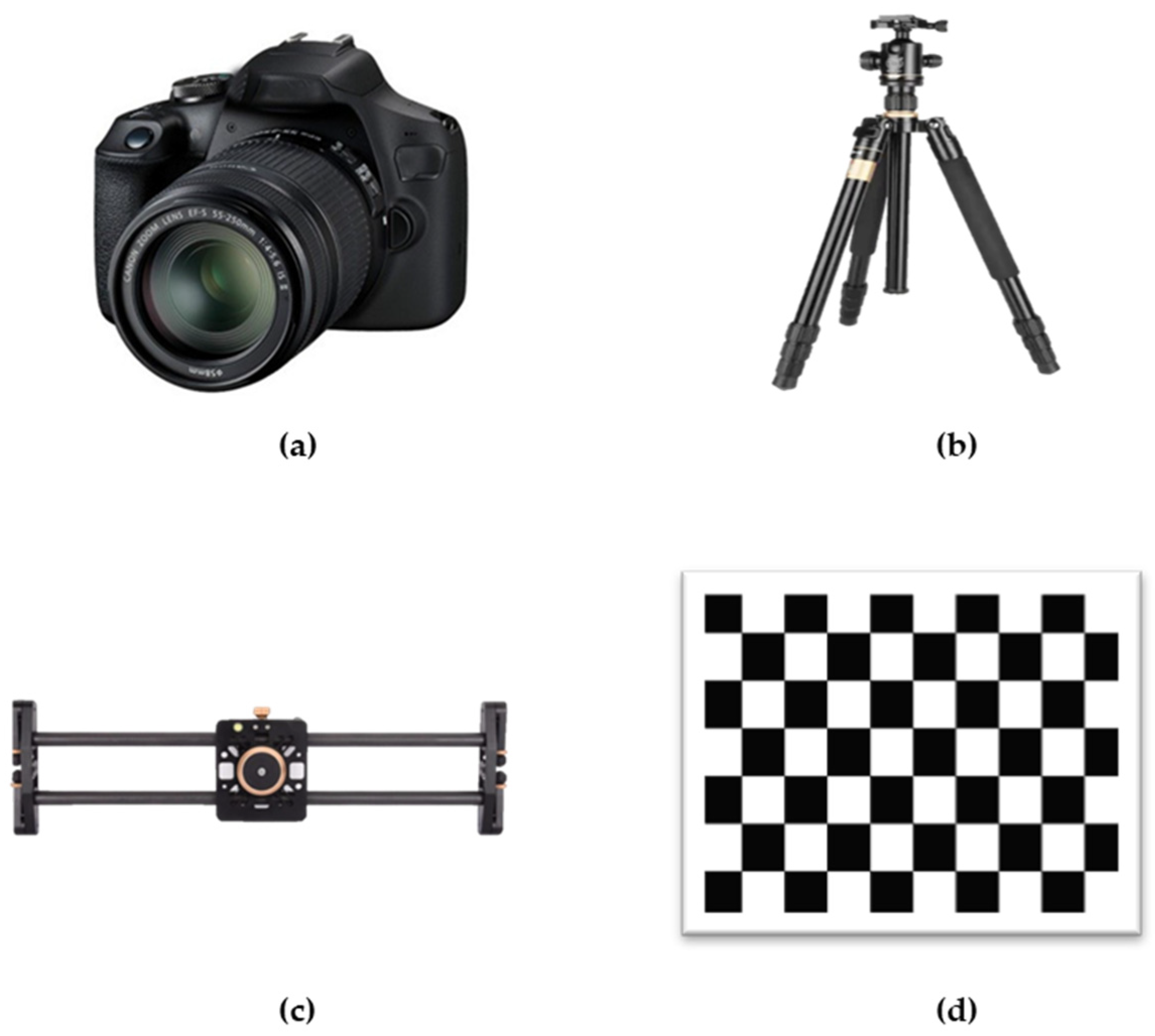
2. Materials
3. Monitoring Methods
3.1. Digital Camera Calibration
3.2. Sub-Pixel Algorithm for Calculating Coordinates of Center of Ring Mark
3.2.1. Marks of Monitoring Points
3.2.2. Sub-Pixel Corner Detection
3.2.3. Least-Square Fitting Center Coordinates
3.3. Calculation of Slope Displacement
4. Results
4.1. Camera Fixation
4.2. Camera Movement
5. Discussion
- (1)
- The relative position of the camera and the slope changed because of the real-time displacement of the slope. The proportional coefficient in this study was the mean value of the two moments, and thus the calculated displacement of the slope had a certain error. Therefore, the time difference between the two proportional coefficients could be shortened to improve the accuracy and obtain more precise displacement values. This method is most suitable for monitoring the large displacement of a slope within a short time.
- (2)
- The accuracy of measurement was similar to the study of Luo and Lin et al. [19,20], reaching the accuracy of millimeters. However, this study took into account the changing position of the digital camera, and the result was accurate to the millimeter level, too. The calibration of the digital camera was not considered in the study by Lin [19]. For non-metric digital cameras, the camera calibration directly affects the accuracy of measurement results. The Zhang Zhengyou calibration method is convenient; however, its robustness is not as good as in the space resection method. Therefore, a better distortion parameter solution method and correction model could be used for camera calibration to improve measurement accuracy. On the simulated slope, when the distance was 20 m, the accuracy achieved approximately 2 mm on the X and Z axes and ~10 mm on the Y axis.
- (3)
- During the temporary placement of the digital cameras and landmarks on the test day, the field error was large due to the influence of external weather factors. Several improvement measures can be taken for the test device: constructing a pan-tilt camera to ensure stability, using steel landmarks for the deeply buried slope of the concrete foundations, and using better image-processing algorithms to calculate the center coordinates of landmarks. In this study, the slope displacement value was obtained by processing the images. The temporal resolution could be increased by shooting a monitoring video, and the data could be transmitted and processed in real time. The specific displacement and velocity of the slope could thus be calculated, and an early warning device could be installed.
6. Conclusions
- (1)
- The designed ring mark points were used as monitoring marks. Compared with the traditional mark points, more corners could be calculated using the circular contour sub-pixel algorithm. In addition, based on the Harris corner detection algorithm, the Shi–Tomasi method was used to calculate the corner points, and the cornerSubPix() function in OpenCV was used to calculate the sub-pixel coordinates of the corner points. Then, the least-square method was used to fit the sub-pixel coordinates of the center of the ring marks, which improved the accuracy of the center coordinates.
- (2)
- Slope-monitoring technology based on the sub-pixel ring mark of a non-metric camera overcomes cumbersome and internal data processing and high specialization requirements, facilitates restriction by terrain, and avoids expensive hardware equipment required in common methods. Simultaneously, when the displacement of the digital camera is known, the displacement of the slope can also be obtained. Moreover, the monitoring accuracy of this method can reach the millimeter level. This method can be used in building deformation monitoring, slope monitoring, etc. Further work will focus on improving temporal resolution by shooting a monitoring video, and the data can be transmitted and processed in real time.
Author Contributions
Funding
Institutional Review Board Statement
Informed Consent Statement
Acknowledgments
Conflicts of Interest
References
- Bai, Y. Comparison of several optical measurement methods applied to measure displacement of test model. Rock Soil Mech. 2009, 30, 2783–2786. [Google Scholar]
- Chen, W.; Li, X.; Wang, Y.; Chen, G.; Liu, S. Forested landslide detection using LiDAR data and the random forest algorithm: A case study of the Three Gorges. Remote Sens. Environ. 2009, 152, 291–301. [Google Scholar] [CrossRef]
- Lian, X.; Li, Z.; Yuan, H.; Hu, H.; Cai, Y.; Liu, X. Determination of the stability of high-steep slopes by global navigation satellite system (GNSS) real-time monitoring in long wall mining. Appl. Sci. 2020, 10, 1952. [Google Scholar] [CrossRef] [Green Version]
- Li, Z.; Song, C.; Yu, C. Application of satellite radar remote sensing to landslide detection and monitoring: Challenges and solutions. Geomat. Inf. Sci. Wuhan Univ. 2019, 44, 967–979. [Google Scholar]
- Feng, W. Close Range Photogrammetry: Photographic Determination of the Shape and Motion of an Object, 1st ed.; Wuhan University Press: Wuhan, China, 2002; pp. 10–30. [Google Scholar]
- Aldao, E.; Gonzalez-Jorge, H.; Pérez, J.A. Metrological comparison of LiDAR and photogrammetric systems for deformation monitoring of aerospace parts. Measurement 2021, 174, 109037. [Google Scholar] [CrossRef]
- Vilbig, J.; Sagan, V.; Bodine, C. Archaeological surveying with airborne LiDAR and UAV photogrammetry: A comparative analysis at Cahokia Mounds. Sci. Rep. 2020, 33, 102509. [Google Scholar] [CrossRef]
- Suziedelyte-Visockiene, J.; Bagdziunaite, R.; Malys, N. Close-range photogrammetry enables documentation of environment-induced deformation of architectural heritage. Environ. Eng. Manag. 2015, 14, 1371–1381. [Google Scholar]
- Jiang, R.; Jáuregu, D.; White, K. Close-range photogrammetry applications in bridge measurement: Literature review. Measurement 2008, 41, 823–834. [Google Scholar] [CrossRef]
- Choi, H.; Ahn, C.; Hong, S. The application of digital close-range photogrammetric linkage to navigation system. J. Korean Soc. Surv. Geod. Photogramm. Cartogr. 2008, 36, 465–473. [Google Scholar]
- Song, L.; Zhang, C.; Bi, J.; Fang, S.; Wang, B.; Gu, S.; Wang, D.; Wang, H. Locating method of close-range photogrammetry based on GPS. Sci. Surv. Mapp. 2011, 36, 40–41. [Google Scholar]
- Hwang, J.; Yun, H.; Kang, J. Development of close range photogrammetric model for measuring the size of objects. KSCE J. Civ. Environ. Eng. Res. 2009, 29, 129–134. [Google Scholar]
- Matori, A.; Mokhtar, M.; Cahyono, B.; Yusof, K. Close-range photogrammetric data for landslide monitoring on slope area. In Proceedings of the 2012 IEEE Colloquium on Humanities, Science & Engineering, Kota Kinabalu, Malaysia, 27 May 2013. [Google Scholar]
- Alameda-Hernández, P.; Hamdouni, R.; Irigaray, C.; Chacón, J. Weak foliated rock slope stability analysis with ultra-close-range terrestrial digital photogrammetry. Bull. Eng. Geol. Environ. 2019, 78, 1157–1171. [Google Scholar] [CrossRef]
- Kim, D.; Gratchev, I.; Berends, J.; Balasubramaniam, A. Calibration of restitution coefficients using rockfall simulations based on 3D photogrammetry model: A case study. Nat. Hazards 2015, 78, 1931–1946. [Google Scholar] [CrossRef] [Green Version]
- Stylianidis, E.; Patias, P.; Tsioukas, V. A digital close-range photogrammetric technique for monitoring slope displacements. In Proceedings of the 11th FIG Symposium on Deformation Measurements, Santorini, Greece, 25 May 2003. [Google Scholar]
- Zhang, C.; Zha, C.; Zhou, S. 3D Visualization of landslide based on close-range photogrammetry. Instrum. Mes. Metrol. 2019, 18, 479–484. [Google Scholar] [CrossRef]
- Ohnishi, Y.; Nishiyama, S.; Yano, T.; Matsuyama, H.; Amano, K. A study of the application of digital photogrammetry to slope monitoring systems. Int. J. Rock Mech. Min. 2006, 43, 756–766. [Google Scholar] [CrossRef]
- Lin, X. Study on Application of Ordinary Digital Cameras in Detection of Engineering. Master’s Thesis, Zhejiang University, Hangzhou, China, 2008. [Google Scholar]
- Luo, R.; Liu, X. A Study of the application of digital photogrammetry in slope deformation monitoring. J. Shijiazhuang Railw. Inst. 2011, 24, 69–74. [Google Scholar]
- Zhang, Z. A flexible new technique for camera calibration. IEEE Trans. Pattern Anal. Mach. Intell. 2000, 22, 1330–1334. [Google Scholar] [CrossRef] [Green Version]
- Harris, C.; Stephens, M. A combined corner and edge detector. Alvey Vis. Conf. 1988, 15, 10-5244. [Google Scholar]
- Shi, J.; Tomasi, C. Good Features to Track. In Proceedings of the IEEE Conference on Computer Vision and Pattern Recognition, Seattle, WA, USA, 21 June 1994. [Google Scholar]
- Zhong, H.; Ye, J.; He, G. Optimization design of center coordinates location based on OpenCV. Test Qual. 2021, 5, 110–115. [Google Scholar]
- He, G.; Luo, H.; Wang, Y. Applicability of slope superficial displacement monitoring by ordinary digital camera. China Energy Environ. Prot. 2018, 40, 88–93. [Google Scholar]


| Content | Value |
|---|---|
| Model | EOS 1500D |
| Sensor type | CMOS |
| Focal length (mm) | 55 |
| Sensor size (mm) | 22.3 × 14.9 |
| Photo resolution (pixels) | 6000 × 4000 |
| Calibration Content | Calibration Value |
|---|---|
| Principal point (pixels) | 2828.054 |
| Principal point (pixels) | 2296.051 |
| Focal length (pixels) | 14025.32 |
| Radial distortion | 0.21835 |
| Radial distortion | −8.12935 |
| Radial distortion | 0 |
| Tangential distortion | 0.00690 |
| Tangential distortion | −0.00825 |
Publisher’s Note: MDPI stays neutral with regard to jurisdictional claims in published maps and institutional affiliations. |
© 2022 by the authors. Licensee MDPI, Basel, Switzerland. This article is an open access article distributed under the terms and conditions of the Creative Commons Attribution (CC BY) license (https://creativecommons.org/licenses/by/4.0/).
Share and Cite
Han, Y.; Lian, X.; Wang, F.; Fan, H. Non-Measuring Camera Monitoring of Comprehensive Displacement of Simulated Slope Mass Based on Edge Extraction of Subpixel Ring Mark. Appl. Sci. 2022, 12, 3966. https://doi.org/10.3390/app12083966
Han Y, Lian X, Wang F, Fan H. Non-Measuring Camera Monitoring of Comprehensive Displacement of Simulated Slope Mass Based on Edge Extraction of Subpixel Ring Mark. Applied Sciences. 2022; 12(8):3966. https://doi.org/10.3390/app12083966
Chicago/Turabian StyleHan, Yu, Xugang Lian, Fan Wang, and Haodi Fan. 2022. "Non-Measuring Camera Monitoring of Comprehensive Displacement of Simulated Slope Mass Based on Edge Extraction of Subpixel Ring Mark" Applied Sciences 12, no. 8: 3966. https://doi.org/10.3390/app12083966
APA StyleHan, Y., Lian, X., Wang, F., & Fan, H. (2022). Non-Measuring Camera Monitoring of Comprehensive Displacement of Simulated Slope Mass Based on Edge Extraction of Subpixel Ring Mark. Applied Sciences, 12(8), 3966. https://doi.org/10.3390/app12083966