Article

Uniform Accuracy Lifetime Principle and Optimal Design Methods for Measurement Systems

School of Instrument Science and Opto-Electronics Engineering, Hefei University of Technology, Hefei 230009, China
*
Author to whom correspondence should be addressed.
Appl. Sci. 2022, 12(8), 3961; https://doi.org/10.3390/app12083961
Submission received: 10 March 2022 / Revised: 11 April 2022 / Accepted: 13 April 2022 / Published: 14 April 2022
(This article belongs to the Special Issue Precision Manufacturing and Intelligent Machine Tools)

Abstract

:
The accuracy of measurement instruments, as well as that of their components, gradually declines as time goes on. Due to different loss mechanisms and the allowable accuracy loss values, the accuracy lifetimes of a whole system and its components are generally nonuniform, which lead to the waste of resources and costs. In this paper, a novel design method based on the uniform accuracy lifetime principle is presented to avoid the waste of resources. After giving and determining the uniformity and accuracy loss weights, optimal design models are established, and the sequential quadratic programming (SQP) method is employed to solve the models. A design example is presented to verify the effectiveness of the design model and the solution method. Using this method, the minimum accuracy lifetime of the whole system extends from 73.07 weeks to 200 weeks, and the uniformity improves from 0.75 to 0.96. The proposed method can be used in practice to achieve the target of uniform accuracy lifetimes for measurement systems because it is easy for manufacturers to obtain the average loss velocities of different components. The implementation of the optimization method will greatly help to save resources and improve the utilization efficiency of instruments or equipment.

1. Introduction

Measurement accuracy is one of the most important indexes of a measurement system. However, it has been discovered in practice that measurement accuracy is not always constant and that it gradually declines as time goes on [1]. This phenomenon is called “accuracy loss”. In general, a measurement system often has some components. The accuracy loss of the whole system is a comprehensive result of that of each component. Due to difference principles, structures and parameters, the accuracy loss laws of components are generally different. Once the accuracy loss value exceeds the allowable value, the component is considered as “failure in accuracy”. There are two situations that can occur in a measurement system: one is that the whole system does not fail in accuracy but some components do, and the other is that the system fails in accuracy but some components do not. Whether the system or its components fail in accuracy, the whole system would be unable to perform normal measurement functions. The emergence of either of these two situations leads to the waste of effective equipment resources and costs. If designers pay attention to the accuracy loss laws of the designed system and its components, and make the accuracy loss values reach their allowable values at the same time, the system can be optimally designed to save resources and costs as much as possible.
Much work has been carried out on the accuracy loss laws of some typical systems with mechanical structures, such as screw balls, linear guides, mechanical wear and sensors [2,3,4,5,6,7,8,9,10,11,12]. J.L. Liu et al. considered the combined effect of intermittent contact between balls and screw grooves, as well as the multiscale contact effect of surface microtopography, and a modified Archard wear model was proposed to investigate the precision loss [2]. In the stable wear stage, the error between the measured data and the predicted precision loss value was less than 11.94%. J.J. Zhao et al. conducted a study on the contact wear of a double-nut ball screw, and a precision loss model was established based on raceway fractal characteristics and a full ball load distribution theory [3]. B.B. Qi and Q. Cheng et al. studied the precision loss law of ball screws under the sliding/rolling mixed motion mode [4,5]. The precision loss rate was the maximum when the screw rotation speed was 40 r/min and the axial load was 4000 N. K.C. Fan et al. proposed a mathematical model to calculate the geometric errors of sliding due to contact deformation and then predicted the positioning errors after long-term operation [6]. To describe the precision loss law of linear ball guides under load conditions, Y. Zhong et al. proposed a wear loss model based on the Hertz contact theory and Archard wear theory [8]. M.L. Jiang et al. studied the accuracy loss laws of main units in a pressure sensing system, and a precision loss model was built based on a neural network (NN) [9]. Moreover, M.L. Jiang et al. also employed a support vector machine (SVM), an artificial neural network (ANN) and wavelet analysis (WA) to model and forecast the measurement accuracy loss laws [11,12]. Based on the awareness that the performance of measurement systems will continuously degrade with time, some scholars are committed to developing lifetime prediction methods of mechanical structures [13,14,15,16,17]. X.C. Zhang et al. proposed a screw lifetime prediction method based on a wavelet neural network (WNN) and empirical mode decomposition (EMD) [13]. To predict the performance degradation trend of rolling bears, Z.C. Xu et al. proposed a lifetime prediction method based on an improved regression support vector machine (SVR) [14]. The prediction results of the proposed method are better than those of common methods. Y.Y. Cheng et al. aimed to establish the pre-relationship and post-relationship of time series in NN and a way to update weights, and a prediction method of a rotating machine’s residual useful lifetime was proposed based on a quantum gene chain coding bidirectional neural network [17]. For some key components of mechanical equipment, the accuracy loss can be forecasted and the lifetime can be predicted using the above methods. However, the above studies mainly focus on the accuracy loss and lifetime prediction of a single structure or part. Most measurement systems consist of several components. Moreover, the accuracy loss laws and the accuracy lifetimes of a system and its components are often different, which lead to the inefficient use of instruments and to the wasting of effective resources and costs. Therefore, further investigation is still required to equalize the accuracy loss law of each component and to achieve uniformity of systems’ accuracy lifetimes.
Equalization designs have attracted great attention in the fields of electronics and networks [18,19,20,21]. In addition to the equalization designs of the circuit, voltage and energy at any given moment, there are some equalization strategies for the whole group’s lifetime [22,23,24,25]. Due to inconsistency among the battery cells of electric vehicles, Z.Y. Dai et al. proposed a hybrid optimal control scheme, in which the voltage balancing mode was enabled after completing capacity equalization [22]. To achieve a better battery pack cycle life, Y.X. Wang et al. proposed a lifetime equalization strategy aiming to optimize the worst cell’s working range [24]. However, for mechanical structures or systems, few studies consider the accuracy loss relationship between the whole system and its components. To solve this problem, Y.T. Fei et al. proposed a novel uniform design theory based on the “white” error model of the total system [26]. Based on this theory, M.L. Jiang et al. obtained the weight functions of the accuracy loss of each main structural component using the grey correlation analysis method [27]. The main cause of the accuracy loss of the whole system was found. F.F. Liu et al. established a uniform loss theoretical model to direct the uniform loss design according to a principle of equality life design [28]. Nevertheless, identifying how to establish a universal design model based on the uniform accuracy life principle is still an unsolved problem. A novel optimal design model for measurement systems based on the uniform accuracy life principle is established and solved in this paper. The optimal models and the solution method can be used to provide some practical guidance to the uniform design of an actual measurement system and save resources and costs. This paper is organized as follows: Section 2 outlines the principle of uniform accuracy lifetime design, and the optimal design is described in detail in Section 3. In Section 4, a design example is given to verify the effectiveness of the optimal design method, and conclusions are drawn in Section 5.

2. The Principle of Uniform Accuracy Lifetime Design

2.1. The Principle

Suppose the number of components in a measurement system is n, δs(t) is the accuracy loss function of the whole system at time t and δi(t) is that of the i-th component. If their accuracy loss allowable values are known as δΔs, δΔ1, δΔ2, …, δΔn, the accuracy lifetime of the system Ts and that of each component Ti can be calculated using the following equations:
δ s ( t ) | t = T s = δ Δ s ,   δ i ( t ) | t = T i = δ Δ i   ( i = 1 , 2 , , n ) .
Hence,
T s = G s 1 [ δ s ( t ) ] | δ ( T S ) = δ Δ S ,   T i = G i 1 [ δ i ( t ) ] | δ i ( T i ) = δ Δ i ,
where G−1 represents the inverse function of the corresponding loss function. If the accuracy lifetimes of each component and the whole system are equal to each other, that is, T1 = T2 = … = Tn = Ts, the system is absolutely uniform in its accuracy lifetime and does not waste resources. Otherwise, if T1T2 ≠ … ≠ TnTs, the accuracy loss functions δs(t), δ1(t), δ2(t), …, δn(t) should be rationally designed and modified to achieve a uniform accuracy lifetime.

2.2. Definition of Uniformity of the Accuracy Lifetimes

According to the uniform accuracy lifetime principle, accuracy lifetimes should be absolutely equal to each other. However, this is impossible for an actual measurement system due to some uncontrollable influencing factors. A certain variation in lifetimes should be allowed in a specific design process. In order to establish a practical uniform design model, the uniformity ρ, which characterizes the variation in lifetimes, should be given. Referring to the definition of the uniformity of illuminance [29], the uniformity ρ of the measurement system can be defined as follows:
ρ = min { T 1 , T 2 , , T n , T s } T ¯ , T ¯ = i = 1 n T i + T s n + 1 .
Obviously, when the minimum lifetime min {T1, T2, …, Tn, Ts} of the whole system is equal to the mean lifetime T ¯ , then ρ = 1, and the whole system is absolutely uniform; when min {T1, T2, …, Tn, Ts} is equal to 0 and far from T ¯ , then ρ = 0, and the uniformity of the system is the worst. The smaller ρ, the worse the accuracy lifetime uniformity, and the system should be improved. On the contrary, the bigger ρ, the better the accuracy lifetime uniformity. If ρ is bigger than the expected value, the measurement system can be regarded as basically uniform.
For an actual measurement system, the lifetimes of the system and its components are generally different from each other. After obtaining each lifetime, the uniformity of the whole system ρ can be calculated. If ρ is smaller than the required uniformity index ε of the measurement system, the accuracy loss laws of some components should be redesigned. Here, ε can be determined according to the service life, the cost of budget for the system etc.

2.3. Definition and Determination of the Accuracy Loss Weight

To achieve the optimal design of the accuracy lifetimes of a measurement system, the accuracy loss functions of components should be rationally changed. However, there are two problems that should first be solved: (1) What are the main components that affect the accuracy loss of the system? (2) When the accuracy loss of the main components changes, what are the impacts on the whole system?
To solve the above two problems, the accuracy loss weight is proposed. In our opinion, the accuracy loss weight should express the influence coefficient of each component’s accuracy loss characteristic on that of the whole system. The greater the accuracy loss weight, the greater the effect of the corresponding component on the whole system. This component should be considered in advance to improve its accuracy loss law. When the accuracy loss weight is small enough, the accuracy loss of the corresponding component can be ignored, and the design model can be simplified. In order to determine the main parameters to be designed and to establish the optimization model, the accuracy loss weight of each component should be calculated.
For a measurement system with n components, the accuracy loss δs(t) of the whole system can be expressed as follows:
δ s ( t ) = p 1 δ 1 ( t ) + p 2 δ 2 ( t ) + + p n δ n ( t ) ,
where pi is the accuracy loss weight of the i-th component. Suppose that the accuracy loss data at different times ti (i = 1, 2, …, m) are obtained through dynamic accuracy loss experiments: {δs(t), δ1(t), δ2(t), …, δn(t)}. According to the definition of the accuracy loss weight, the multiple linear regression method can be adopted to estimate the accuracy loss weight pi.
Defining
Y = [ δ s ( t 1 ) δ s ( t 2 ) δ s ( t m ) ] ,   X = [ δ 1 ( t 1 ) δ 2 ( t 1 ) δ n ( t 1 ) δ 1 ( t 2 ) δ 2 ( t 2 ) δ n ( t 2 ) δ 1 ( t m ) δ 2 ( t m ) δ n ( t m ) ] ,   P = [ p 1 p 2 p n ] ,
the best estimated value of the accuracy loss weight pi in matrix form can be obtained in terms of the least-squares principle:
P ^ = [ p ^ 1 p ^ 2   p ^ n ] = ( X T X ) 1 X T Y .
In accordance with the principle of uniformity design of accuracy lifetimes, the redesigned accuracy loss sequences {δs(t)′, δ1(t)′, δ2(t)′, …, δn(t)′} should satisfy Formula (6):
{ δ ( t ) | t = T s = p 1 ( ) δ 1 ( t ) + p 2 ( ) δ 2 ( t ) + + p n ( ) δ n ( t ) | t = T s = δ Δ s δ 1 ( t ) | t = T 1 = δ Δ 1     δ n ( t ) | t = T n = δ Δ n .
In addition, the updated uniformity ρ′ can be calculated in terms of Formula (3). Meanwhile, ρ′ should meet the inequation ρ′ ≥ ε. After optimization, the uniformity design of accuracy lifetimes can be realized in the system.

3. Optimization Modeling for the Uniformity Design of Accuracy Lifetimes

To establish the optimization model, the design variables and their constraints and objective functions should be determined, and an appropriate algorithm to obtain the optimal solutions should also be illustrated.

3.1. Determination of Design Variables

The objects to be designed are the accuracy loss laws of the system and its components. However, these time-varying accuracy loss functions have too many variables to be designed. It is unrealistic to use the accuracy loss functions as design variables.
For general engineering designers, it is relatively easy to gain the average velocities Δ v ¯ e i (i = 1, 2, …, n) of the accuracy loss of some components under their working conditions. Therefore, the average velocity of the accuracy loss of each component is taken as a design variable in the optimization model, and the measurement system can be improved according to the designed values Δ v ¯ e i .

3.2. Selection of Objective Functions

In the optimization model of uniform design, the target parameters can be the uniformity ρ′ of lifetimes, accuracy lifetime T′, total improvement cost Cs etc. The target functions are listed as follows:
(1)
The uniformity of lifetimes is the maximum:
max   ρ .
(2)
The effective accuracy lifetime T′ of the measurement system is the maximum. Assuming that the effective lifetime of the system equals the minimum lifetime of all, the objective function is as follows:
max   T = min { T 1 , T 2 , , T n , T s } .
(3)
The total improvement cost Cs is the minimum. Suppose that the relationship between the improvement cost Ci and the designed value Δ v ¯ e i of the i-th component is C i = f i ( Δ v ¯ e i ) , the objective function can be derived:
min   C s = i = 1 n C i = i = 1 n f i ( Δ v ¯ e i ) .
Sometimes, designers are concerned with more than one objective. For instance, when the maximum uniformity with minimal improvement cost is required, the objective function may be established as follows:
max   ρ + 1 C s .
This is suitable for other cases.

3.3. Modeling of Constraint Conditions

First, the constraint conditions of the designed values Δ v ¯ e i should be determined. The accuracy loss velocity of every component is closely related to factors such as the structures, materials and working conditions. For some common or typical components, these factors generally vary within a certain range. Therefore, the average loss velocity of each designed variable Δ v ¯ e i can be limited to a certain range:
Δ v ¯ e i 1 Δ v ¯ e i Δ v ¯ e i 2 .
Here, Δ v ¯ e i 1 and Δ v ¯ e i 2 are the lower bound and the upper bound, respectively, which are determined by the allowable structures, materials and working conditions of every component.
Then, the relationships between the average loss velocity of each designed variable Δ v ¯ e i , lifetime Ti′ and the accuracy loss allowable value δΔi should be investigated:
{ Δ v e 1 T 1 = δ Δ 1 Δ v e 2 T 2 = δ Δ 2     Δ v e 2 T 2 = δ Δ n Δ v e s T s = [ p 1 Δ v e 1 + p 2 Δ v e 2 + + p n Δ v e n ] T s = δ Δ s .
Here, δΔi should be known. In addition, ρ′ should be bigger than the required uniformity; that is,
ρ ε .
There may be other constraint conditions. For example, the total improvement cost should be less than C; that is, C s = i = 1 n C i C . Another example is that the accuracy lifetime of a system should reach the designed lifetime T0; that is, T′ ≥ T0. In brief, the objective functions and constraint conditions should be selected according to the specific conditions of the measurement systems, design requirements and implementation difficulties.

3.4. Solution of the Optimization Model

The optimization design model, which is based on the principle of uniform accuracy lifetime, is often nonlinear and has some constraint conditions. The method of sequential quadratic programming (SQP) is one of the best algorithms to solve these kinds of problems [30]. SQP is adopted to solve this optimization model. First, in terms of the original nonlinear optimization model, the Lagrange function is constructed as an approximate solution. Then, the function is approximated to a quadratic function. Therefore, the original optimization model can be simplified as a quadratic programming problem. Finally, the optimal solution obtained by the quadratic programming problem is that of the original optimization model.
However, the problem of the local optimal solution will appear due to the improper selection of initial values when using the SQP method. To solve this problem, a method combining uniform sampling technology with SQP is proposed in this paper. The solving process can be carried out according to the following steps:
Step 1: employ uniform sampling technology to construct a large number of initial values of the vector Xi (i = 1, 2, …, M), which is composed of the design variables uniformly distributed in the constrained interval.
Step 2: use the SQP method to find the local optimal solution corresponding to the initial value of the i-th group.
Step 3: search for the global optimal solution from a large number of local optimal solutions and obtain the global optimal solution, as well as the corresponding optimal design vector.

4. An Optimal Design

4.1. Design Procedure Based on the Principle of Uniform Accuracy Lifetimes

The optimal design based on the principle of uniform accuracy lifetimes can be achieved by the following steps:
(1)
Obtain the accuracy loss sequences of the measurement system and its components through experiences or experiments, and determine their accuracy loss allowable values.
(2)
Set up models for all accuracy loss sequences, obtain their mathematic functions, and then calculate their original accuracy lifetimes {T1, T2, …, Tn, Ts} according to their accuracy loss allowable values.
(3)
Calculate the uniformity ρ of the lifetime of the whole system, and judge whether it meets the requirement ρε. If ρε, the system does not need to be redesigned. If not, the system should be optimally designed.
(4)
Determine the accuracy loss weights of the components, and establish the optimal design model with an objective function, such as the longest lifetime, the lowest cost or the biggest uniformity (see Section 2).
(5)
Employ the method of combining uniform sampling technology with SQP to solve the optimization model, and then gain the optimal average accuracy loss velocities of the system and its components (see Section 3).
(6)
On the premise of mastering a large number of test data and accuracy loss laws of typical structures, gradually change some factors such as the structures, parameters, materials and working conditions of the original system according to the above designed results until the uniformity design target is achieved.

4.2. A Design Example

Suppose that a measurement system consists of two components, whose accuracies are gradually declining. The accuracy loss values of the whole system and those of the two components (tested once a week) are given over the course of one hundred weeks, as shown in Figure 1.
The accuracy loss weight for each component can be calculated using the multiple linear regression method; that is, p1 = 1.998 for component one, and p2 = 0.475 for component two. Their accuracy loss functions δ1(t), δ2(t), and δs(t) (t > 0) can also be gained by using the least-squares fitting method:
{ δ 1 ( t ) = 0.0031 t 2 + 0.043 t + 0.3052 δ 2 ( t ) = 0.0011 t 2 + 0.0925 t + 0.3232 δ s ( t ) = 0.0066 t 2 + 0.0526 t + 0.7633 .
Meanwhile, the allowable values of the accuracy loss of the system and its components are supposed as δ1 = 20 μm, δ2 = 30 μm and δs = 60 μm, which should be determined according to the different measurement accuracy requirements. Then, the values of the accuracy lifetimes and the uniformity of the system can be calculated as follows:
T 1 73.07   weeks , T 2 127.50   weeks ,   T s 90.84   weeks ,   ρ 0.75 .
Assuming that the uniformity of the system is not big enough and cannot meet the uniformity requirement, the system should be redesigned. Firstly, vector X consisting of the design variables should be determined. Here, the average accuracy loss velocities of component one and component two, Δ v ¯ 1 and Δ v ¯ 2 , respectively, as well as the accuracy lifetimes T1′, T2′ and Ts′, are selected as the design variables. Therefore, the designed vector is
X = ( Δ v ¯ 1 , Δ v ¯ 2 , T 1 , T 2 , T s ) .
Secondly, the optimal design model, including an objective function and constraint conditions, should be established. When the designer focuses on the uniformity of the system, the biggest uniformity can be taken as an objective function:
max   ρ .
For the objective functions, there are two aspects of constraints. One aspect is the variation ranges of the average accuracy loss velocities of component one and component two, Δ v ¯ 1 and Δ v ¯ 2 , respectively. Here, the ranges of the average accuracy loss velocities for component one and component two are both assumed to be between 0.1 μm per week and 0.5 μm per week. In practical applications, the range of the average accuracy loss velocities should be determined by the possible ranges of the loss velocities of different components under the current technical levels and conditions. The other aspect is the boundary constraints of the design parameters, which are determined by the relationships between the accuracy reserves, average accuracy loss velocities and accuracy lifetimes. The total constraint equation is as follows:
s . t .   { Δ v ¯ 1 T 1 = 20 Δ v ¯ 2 T 2 = 30 ( 1.998 Δ v ¯ 1 + 0.475 Δ v ¯ 2 ) T s = 60 0.1 Δ v ¯ 1 0.5 0.1 Δ v ¯ 2 0.5 .
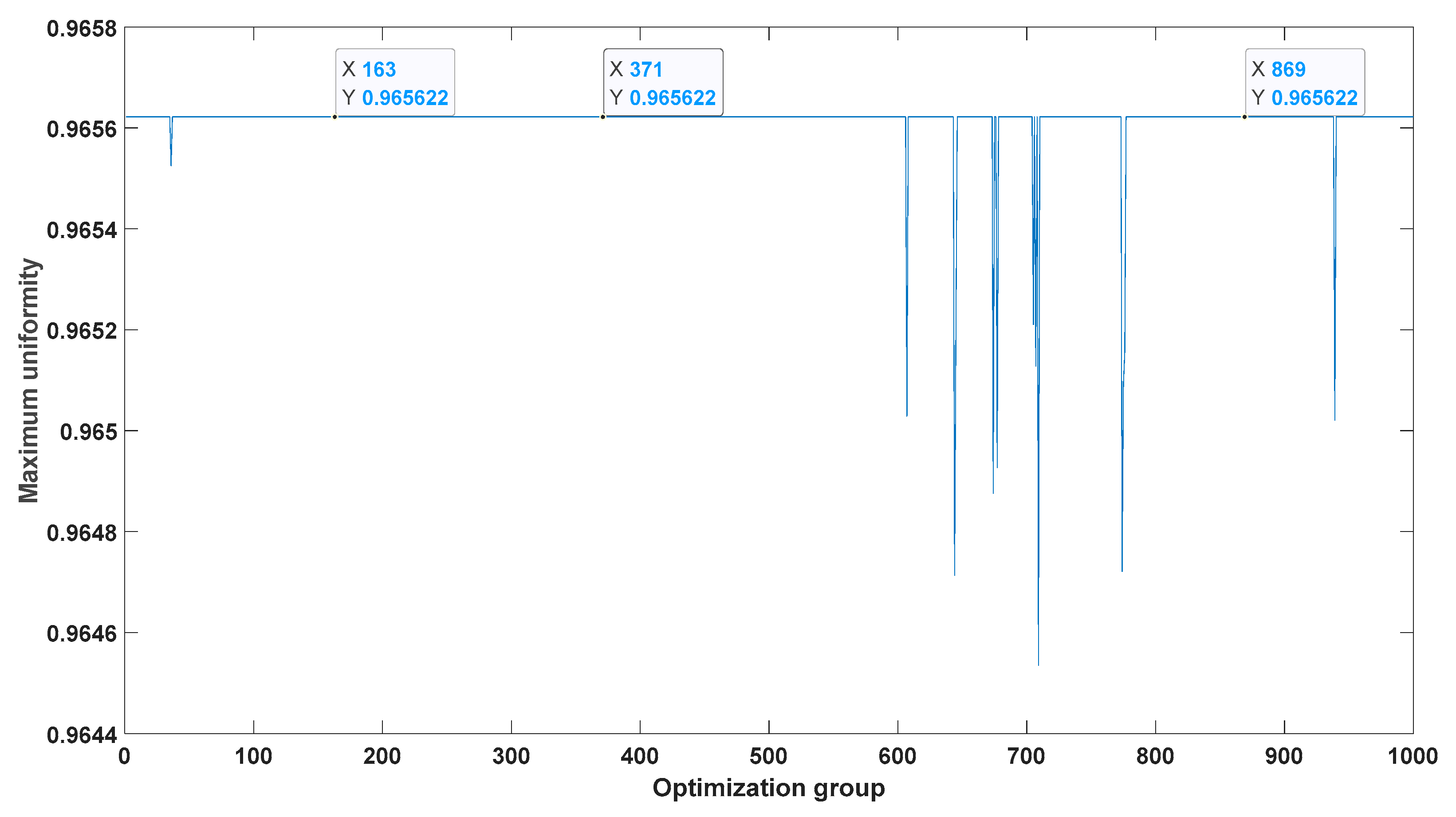
Finally, the optimization model is solved by employing the optimization toolbox in MATLAB. The initial values of 1000 groups uniformly distributed over the range of constraints are generated using uniform sampling. Then, the SQP algorithm is adopted to find the optimum solution in term of the corresponding initial value. Figure 2 shows the optimal solutions of uniformity ρ′ for each group of initial values.
As observed in Figure 2, the optimal solution of uniformity ρmax is
ρ max 0.96 .
There are a great number of optimal design variables corresponding to maximum uniformity. That is, many schemes can be proposed to achieve the goal of maximum uniformity. From the 1000 optimum design variables, it is observed that, as long as the accuracy loss velocities of component one and component two are equal, the optimal solution can be achieved. Suppose that the accuracy loss velocities of component one and component two are the same Δ v ¯ , the following results can be obtained according to the constraint equations:
  ρ max = min { T 1 , T 2 , T s } T ¯ = 20 Δ v ¯ [ 60 ( 1.998 + 0.475 ) Δ v ¯ + 20 Δ v ¯ + 30 Δ v ¯ ] / 3 = 0.96 .
The calculation results verify the effectiveness of the above method. After the optimization design, uniformity improved from the original value of ρ = 0.75 to ρmax = 0.96. Based on these results, system uniformity can be improved if the average loss velocities of the two components are equal to each other. When Δ v ¯ 1 = Δ v ¯ 2 = 0.1 μm per week, the accuracy lifetimes of the whole system and its components are the longest; that is,
T 1 = 200   weeks ,   T 2 = 300   weeks ,   T s = 242.62   weeks .

5. Conclusions

A novel optimal design method based on the uniform accuracy life principle was presented to save resources and improve the utilization efficiency of instruments and equipment. According to the uniform accuracy life principle, the uniformity of the whole system was defined, and the accuracy loss weight of each component was determined using the multiple linear regression method. On this basis, the optimal design models were established according to the different requirements of measurement systems. The combination method of the SQP method and uniform sampling technology was employed to solve these models successfully. The feasibility and effectiveness of the design models and the solution method were verified using an example. The results revealed that the uniformity was improved from the original uniformity of 0.75 to 0.96. When the average loss velocities of the two components were both equal to 0.1 μm per week, the accuracy lifetimes of the whole system and its components (components one and two) were the longest, that is, 242.62 weeks, 200 weeks and 300 weeks, respectively. The uniform principle and the optimal design models can be used to improve the uniformity of accuracy lifetimes for some measurement systems. Further research will focus on the application of the proposed methods to complex instruments and equipment.

Author Contributions

Conceptualization, Z.C. and R.L.; methodology, Z.C.; software, Z.C. and L.L.; validation, Z.C., R.L. and L.L.; formal analysis, R.L.; data curation, Z.C. and L.L.; writing—original draft preparation, Z.C. and L.L.; writing—review and editing, Z.C. and R.L.; project administration, Z.C.; funding acquisition, Z.C. All authors have read and agreed to the published version of the manuscript.

Funding

This research was funded by the National Natural Science Foundation of China, grant number 52175506.

Institutional Review Board Statement

Not applicable.

Informed Consent Statement

Not applicable.

Data Availability Statement

Not applicable.

Conflicts of Interest

The authors declare no conflict of interest.

References

  1. Xie, S.F.; Chen, X.H.; Zhang, Y.B.; Fei, Y.T. The Analysis of Uncertainty and Research of Dynamic Character on Measurement System. Acta Metrol. Sin. 2002, 3, 237–240. [Google Scholar]
  2. Liu, J.L.; Ma, C.; Wang, S.L. Precision loss modeling method of ball screw pair. Mech. Syst. Signal Process 2020, 135, 106397. [Google Scholar] [CrossRef]
  3. Zhao, J.J.; Lin, M.M.; Song, X.C.; Wei, N. A modeling method for predicting the precision loss of the preload double-nut ball screw induced by raceway wear based on fractal theory. Wear 2021, 486–487, 204065. [Google Scholar] [CrossRef]
  4. Qi, B.B.; Cheng, Q.; Li, S.L.; Liu, Z.F.; Yang, C.B. Precision loss of ball screw mechanism under sliding-rolling mixed motion behavior. J. Cent. South Univ. 2021, 28, 1357–1376. [Google Scholar] [CrossRef]
  5. Cheng, Q.; Qi, B.B.; Chu, H.Y.; Zhang, Z.L.; Liu, Z.F.; Zheng, J.G. The analysis on the influence of mixed sliding-rolling motion mode to precision degradation of ball screw. Proc. Inst. Mech. Eng. Part C-J. Mech. Eng. Sci. 2022, 236, 669–688. [Google Scholar] [CrossRef]
  6. Fan, K.C.; Chen, H.M.; Kuo, T.H. Prediction of machining accuracy degradation of machine tools. Precis. Eng.-J. Int. Soc. Precis. Eng. Nanotechnol. 2012, 36, 288–298. [Google Scholar] [CrossRef]
  7. Ji, Z.Q.; Ou, Y.; Feng, H.T.; Zhang, Y. Measurement method and tests for precision-keeping of a linear rolling guide based on online measuring. J. Vib. Shock. 2016, 35, 56–61. [Google Scholar] [CrossRef]
  8. Zhong, Y.; Tao, W.J.; Han, J. Model Study of Precision Loss of Linear Ball Guide. Modul. Mach. Tool Autom. Manuf. Tech. 2013, 12, 33–36. [Google Scholar] [CrossRef]
  9. Jiang, M.L.; Fei, Y.T. The Accuracy Losing Diagnosis about Pressure Sensor System. J. Shanghai Jiaotong Univ. 2006, 12, 2063–2065. [Google Scholar] [CrossRef]
  10. Jiang, M.L. Accuracy losing diagnosis about measuring-system of differential mutual inductive displacement sensor. J. Heilongjiang Inst. Sci. Technol. 2005, 15, 371–373. [Google Scholar] [CrossRef]
  11. Jiang, M.L.; Li, F.P.; Wang, X.D. Dynamic Accuracy Loss Prediction model based on SVM. In Proceedings of the ETP/IITA Conference on System Science and Simulation in Engineering (SSSE 2010), Hong Kong, China, 29 June–1 July 2010. [Google Scholar]
  12. Jiang, M.L.; Wang, X.D.; He, X.H. Dynamic Accuracy Loss Prediction model based on BPNN. In Proceedings of the International Conference on Advanced Measurement and Test (AMT 2010), Sanya, China, 15–16 May 2010. [Google Scholar]
  13. Zhang, X.C.; Gao, H.L.; Huang, H.F.; Zhang, L.; Peng, Z.W. Screw lifetime prediction based on wavelet neural network and empirical mode decomposition. In Proceedings of the International Conference “Vibroengineering—2015”, Nanjing, China, 26–28 September 2015. [Google Scholar]
  14. Xu, Z.C.; Wang, L.J.; Liu, Y.; Cai, K.L.; Chen, Z.K.; Chen, B.J. A Prediction Method for Remaining Life of Rolling Bearing Using Improved Regression Support Vector Machine. J. Xi’an Jiaotong Univ. 2022, 56, 197–205. [Google Scholar] [CrossRef]
  15. Yoo, Y.; Baek, J.G. A Novel Image Feature for the Remaining Useful Lifetime Prediction of Bearings Based on Continuous Wavelet Transform and Convolutional Neural Network. Appl. Sci. 2018, 8, 1102. [Google Scholar] [CrossRef] [Green Version]
  16. Wang, J.B.; Wang, X.H.; Wang, L.Z. Modeling of BN Lifetime Prediction of a System Based on Integrated Multi-Level Information. Sensors 2017, 17, 2123. [Google Scholar] [CrossRef] [Green Version]
  17. Cheng, Y.Y.; Li, F.; Tang, B.P.; Tian, D.Q. Quantum gene chain coding bidirectional neural network for residual useful life prediction of rotating machinery. Chin. J. Sci. Instrum. 2020, 41, 164–174. [Google Scholar] [CrossRef]
  18. Wu, X.G.; Cui, Z.H.; Li, X.F.; Du, J.Y.; Liu, Y. Control Strategy for Active Hierarchical Equalization Circuits of Series Battery Packs. Energies 2019, 12, 2071. [Google Scholar] [CrossRef] [Green Version]
  19. Lewandowski, M.; Bernas, M.; Loska, P.; Szymala, P.; Placzek, B. Extending Lifetime of Wireless Sensor Network in Application to Road Traffic Monitoring. In Proceedings of the 26th International Conference on Computer Networks (CN), Kamien Slaski, Poland, 25–27 June 2019. [Google Scholar]
  20. Hung, L.L. A Smart Sensing and Routing Mechanism for Wireless Sensor Networks. Sensors 2020, 20, 5720. [Google Scholar] [CrossRef]
  21. Yetgin, H.; Cheung, K.T.K.; El-Hajjar, M.; Hanzo, L. A Survey of Network Lifetime Maximization Techniques in Wireless Sensor Networks. IEEE Commun. Surv. Tutor. 2017, 19, 828–854. [Google Scholar] [CrossRef] [Green Version]
  22. Dai, Z.Y.; Liu, Z.R.; Jia, J.H.; Bai, G.; Zhao, X.L. Mixed optimal control scheme based on capacity balance and voltage balance. Power Supply Technol. Its Appl. 2019, 45, 108–112. [Google Scholar] [CrossRef]
  23. Liu, X.H. Life Balance Evaluation System Development of Large Air Separation Compressor Unit. Master’s Thesis, Northeastern University, Shenyang, China, June 2014. [Google Scholar]
  24. Wang, Y.X.; Wei, X.Z.; Fang, Q.H.; Zhu, J.G.; Dai, H.F. Consistency Variation Law and Equalization Strategy of Electric Vehicle Battery for Maximizing the Life of the Battery Pack. J. Mech. Eng. 2020, 56, 176–183. [Google Scholar] [CrossRef]
  25. Wu, D.P. Study on Life Cycle Balancing Strategy of Lithium-ion Power Battery Pack. Master’s Thesis, Chongqing University, Chongqing, China, June 2019. [Google Scholar]
  26. Cheng, Z.Y.; Fei, Y.T.; Chen, X.H. Research on Uniform Design Theory for Dynamic Measurement Systems. China Mech. Eng. 2008, 19, 893–896. [Google Scholar]
  27. Jiang, M.L.; Lu, X.C.; Duan, M.J.; Wang, X.D. Weight function theory of dynamic accuracy loss. In Proceedings of the 7th International Symposium on Precision Engineering Measurements and Instrumentation (ISPEMI), Lijiang, China, 7–11 August 2011. [Google Scholar]
  28. Liu, F.F.; Fei, Y.T.; Jiang, M.L. Theoretical Model of Accuracy Loss Equality Design in Dynamic Measuring System. Trans. Chin. Soc. Agric. Mach. 2008, 39, 134–136. [Google Scholar]
  29. Liao, W.S. Experimental Study on Translucent Concrete Building Components and Indoor Environmental Performance. Master’s Thesis, Dalian University of Technology, Dalian, China, June 2019. [Google Scholar]
  30. Ma, C.F. Optimization Method and Its Matlab Program Design; National Defense Industry Press: Beijing, China, 2010. [Google Scholar]
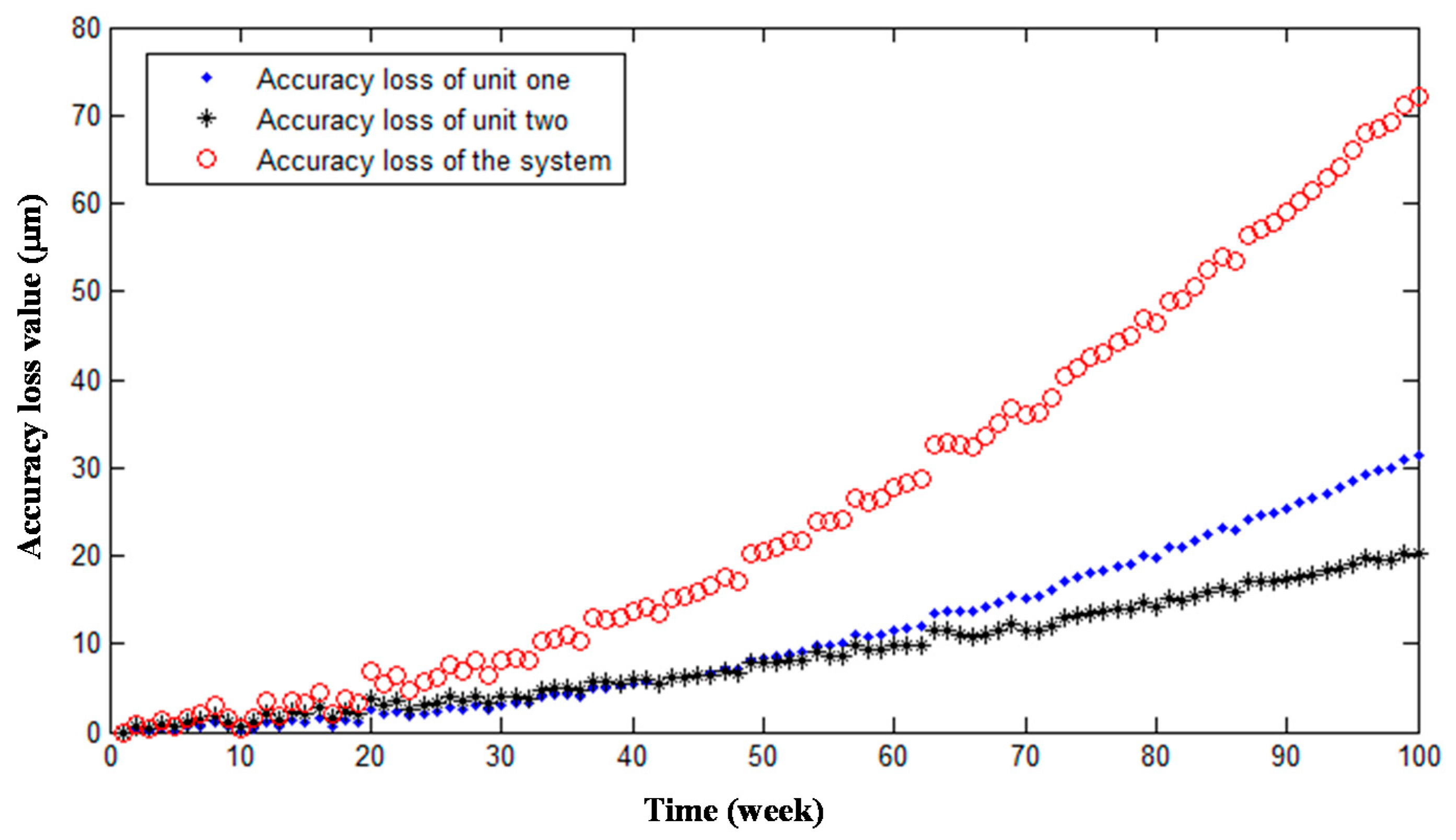
Figure 1. Accuracy loss data of a whole system and its components.
Applsci 12 03961 g001
Figure 2. The optimal solutions of uniformity ρ′ for each group of initial values.
Applsci 12 03961 g002
Publisher’s Note: MDPI stays neutral with regard to jurisdictional claims in published maps and institutional affiliations.