Dynamic Stability Assessment of High-Speed Railway Bridges Using Numerical Model Updating

Abstract

Numerical model updating using the data measured from the actual structure is required in order to minimize the error between the initial numerical model and the actual structure. Field load tests, which are conducted in order to assess the condition and safety of high-speed railway bridges, are generally expensive and restricted by railway control and weather conditions. Therefore, a method for evaluating the performance of high-speed railway bridges using updated numerical models without conducting field load tests is required. In this study, numerical model updating was performed by using the data measured from the ambient vibration test in order to assess the dynamic stability of high-speed railway bridges. In the ambient vibration test, the measurement point roaming method was applied in order to accurately measure high-speed railway bridges using a limited number of sensors. For numerical model updating, the univariate search method was used, and several measured parameters were updated and converted into the properties of the target bridges in the numerical models. The vertical and torsional modes of the updated numerical models differed by less than 5% from those estimated using the data measured from the target bridges. The responses of the updated numerical models were found to be similar to those measured from the high-speed railway bridges in operation. It was also shown that the updated numerical models could be used to assess the dynamic stability of the bridges.

1. Introduction

With the worldwide dissemination of high-speed railways, studies have been conducted in order to maintain high-speed railway structures, such as roadbeds, tracks, overhead systems, and bridges, by using numerical model updating [1,2,3,4]. Since the damage to high-speed railway bridges caused by accidents can be more severe compared to other structures, numerical models that can accurately express the response characteristics of actual structures are very important for performing system identification, damage assessment, and structural health monitoring [5,6,7]. In general, the initial numerical model based on structural design documents is different from the results measured from the high-speed railway bridge [8,9]. The difference is particularly more significant for high-speed railway bridges in operation due to construction errors and deterioration resulting from aging and structural damage [10,11,12]. Therefore, it is necessary to confirm that the deterioration of high-speed railway bridges is within the allowable range and no structural problems exist. Numerical model updating using the results measured from high-speed railway bridges in operation is very important in securing structural safety and performing efficient maintenance [13,14,15]. Reliable numerical model updating can reduce maintenance costs during the service period by recognizing and responding to the deterioration of high-speed railway bridges at an early stage. It can also be used as basic data to perform proper maintenance on significantly deteriorated high-speed railway bridges.

The main methods used to perform numerical model updating are the direct method and the iterative method. The direct method has been developed in a variety of ways since the development of the Lagrange multiplier method [16,17,18,19], matrix mixing method [20,21,22,23], and error matrix method [24,25,26]. The direct method optimizes an objective function with constraints composed of the modal data measured from a structure and the system matrix of a numerical model. System matrix error is prepared as a mathematical function so that it can be corrected with a single calculation. Since the direct method attempts to correct the change in stiffness and mass directly from the mathematical function, accurate model updating is difficult if the structure has a complex degree of freedom. In order to address these issues, iterative methods were developed. Iterative methods can be divided into the sensitivity method that relies on the sensitivity of natural frequency and mode shape to changes in variables to be updated and the sensitivity method that uses the frequency response function of a structure, with the penalty function being mainly used [27,28,29,30,31]. Sensitivity methods can be divided into directly updating the element matrix of the member and updating physical variables. The iterative method that uses the sensitivity matrix is effective in identifying variables, such as materials, geometrical properties, and boundary conditions, that directly affect the dynamic properties of a structure. However, the sensitivity matrix must be prepared for all variables to be updated. The iterative method based on this sensitivity method always requires the differential functions of matrices on dynamic properties, such as natural frequency and mode shape, for each parameter, and its applicability for a complex structure is significantly low. It is also difficult to apply a commercial finite element analysis program due to the complexity of the inverse analysis algorithm. A method of updating the stiffness of the numerical model using displacement response was suggested in order to improve such applicability. However, it was applied to general railway bridges without interaction between the bridge and the train [32]. Most methods that use the iterative method have only been applied to very simple structures, and reduction and expansion of the system matrix is required in order to match the measurement degree of freedom. This demonstrates the limited application of the iterative method to actual structures [33].

To compensate for these shortcomings, iterative methods based on optimization techniques, such as genetic algorithms, have been proposed [34,35,36,37]. Genetic algorithms are random search methods that are designed to stochastically find a solution in the entire space. They are very effective in finding the global optimum point, optimizing continuous and discontinuous variables, and finding an approximate global minimum value despite many local minimum values. As a result, they are very effective in finding the optimal starting point from a number of populations given as random variables in a problem with multiple variables [38]. However, they require more iterative calculations and a longer computation time than the existing methods that use the formulation and differentiation of mathematical models.

This study proposed an iterative method based on the univariate search method [39] that does not require the preparation of differential functions during the numerical model updating stage. The proposed method performed numerical model updating by comparing the response measured from the ambient vibration test using a commercial finite element analysis program with high accessibility. It also enables numerical model updating through a small number of iterations. The applicability and usability of the numerical model updating method were examined by conducting a dynamic stability assessment for high-speed railway bridges using the updated numerical model.

The ambient vibration test provided the response required for the numerical model updating of high-speed railway bridges. For the accurate measurement in the ambient vibration test, it is necessary to acquire responses at many points on high-speed railway bridges. However, the applicable sensors in the field are limited. In terms of load conditions of high-speed railway bridges, the speed and load of high-speed trains hardly change due to the characteristics of the trains. As a result, a measurement point roaming method, which performs multiple measurements while moving a small number of sensors using a wireless measurement system with high field applicability, was applied in this study. The dynamic properties estimated from the response measured using the measurement point roaming method were used as target values for updating the initial numerical model prepared based on the structural design document.

2. Experimental Setup for Ambient Vibration Test

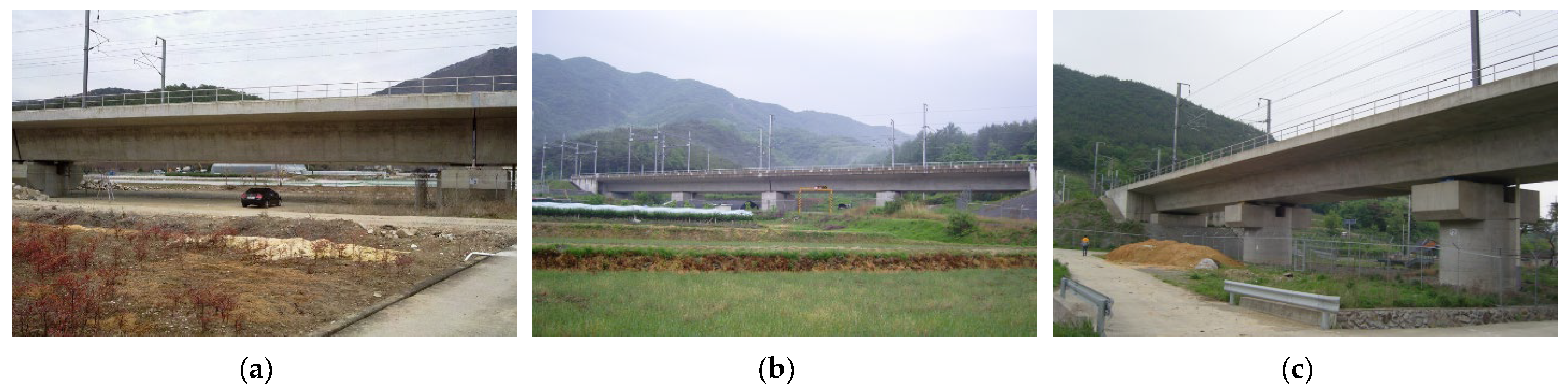
Assessment is performed in order to examine the safety of high-speed railway bridges, and detailed investigations, including load tests, are periodically or additionally performed in order to assess the safety of the bridges. Since it is difficult to conduct field load tests due to various restrictions, a safety assessment method that uses the ambient vibration test is required. Therefore, if periodic load tests can be replaced with the ambient vibration test, the maintenance of high-speed railway bridges will become more efficient and economical.

2.1. Target Bridges

Prestressed concrete (PSC) box girder bridges represent more than 70% of high-speed railway bridges in South Korea. In this study, three PSC box girder bridges (Imgi 2nd Bridge [one span], Maeaji Bridge [two spans], and Hwalchun Bridge [three spans]) were selected as target bridges based on the number of spans. These three bridges were designed to connect Busan, Gyeongju, and Daegu on the Gyeongbu high-speed railway. The Imgi 2nd Bridge consists of 11 girders of 40 m and a single span, and the second span was selected as the target position. The Maeaji Bridge has two continuous girders of 50 m and four spans with a total length of 100 m, and the third and fourth spans were selected as the target positions. The Hwalchun Bridge has one continuous girder of 75 m and three spans. Figure 1 shows the target bridges, while

Table 1. Specifications of the target bridges.

Item	Imgi 2nd Bridge	Maeaji Bridge	Hwalchun Bridge
type	PSC box girder	PSC box girder	PSC box girder
span length	40 m single span 11 girders (440 m)	25 m @2 spans two continuous girders (100 m)	25 m @3 span one continuous girder (75 m)
bridge width	14 m	14 m	14 m
measurement position	second span	third and fourth spans	first to third spans
number of measurement points	34 (four groups)	32 (three groups)	48 (five groups)
measurement time	50 s	50 s	50 s
sampling rate	200 Hz	200 Hz	200 Hz
high-speed train speed	270–300 km/h	270–300 km/h	270–300 km/h

outlines their specifications.

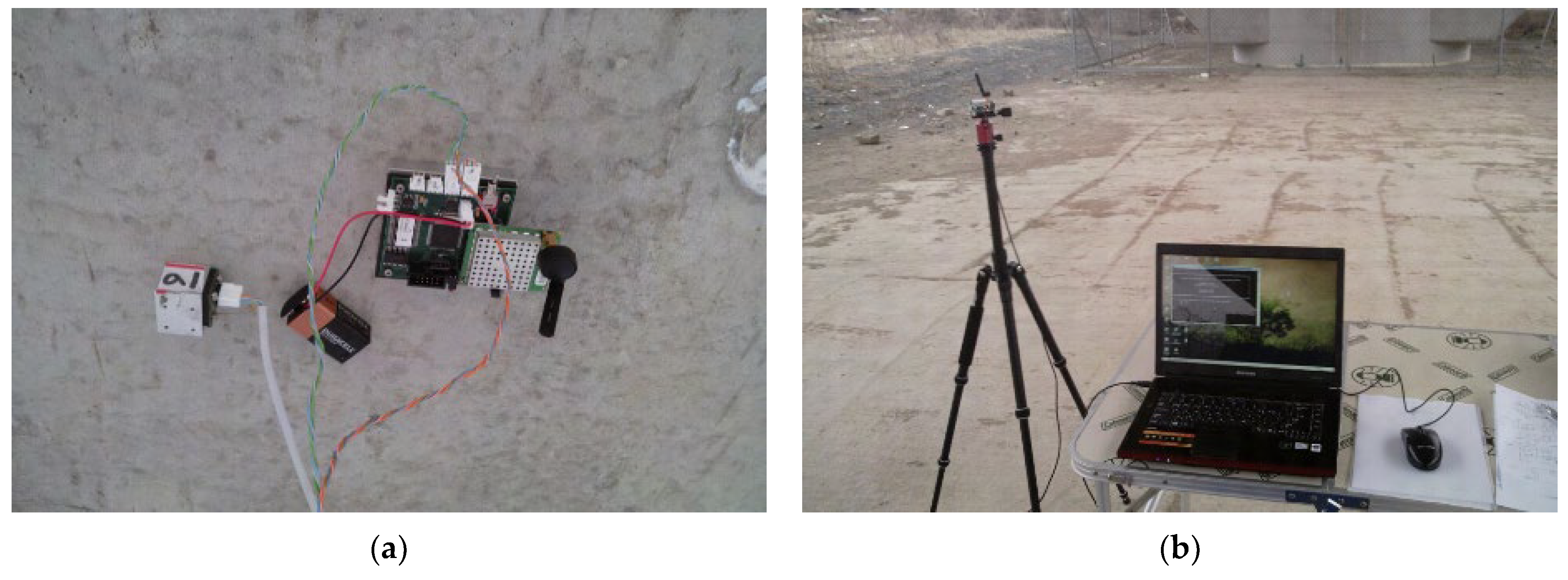
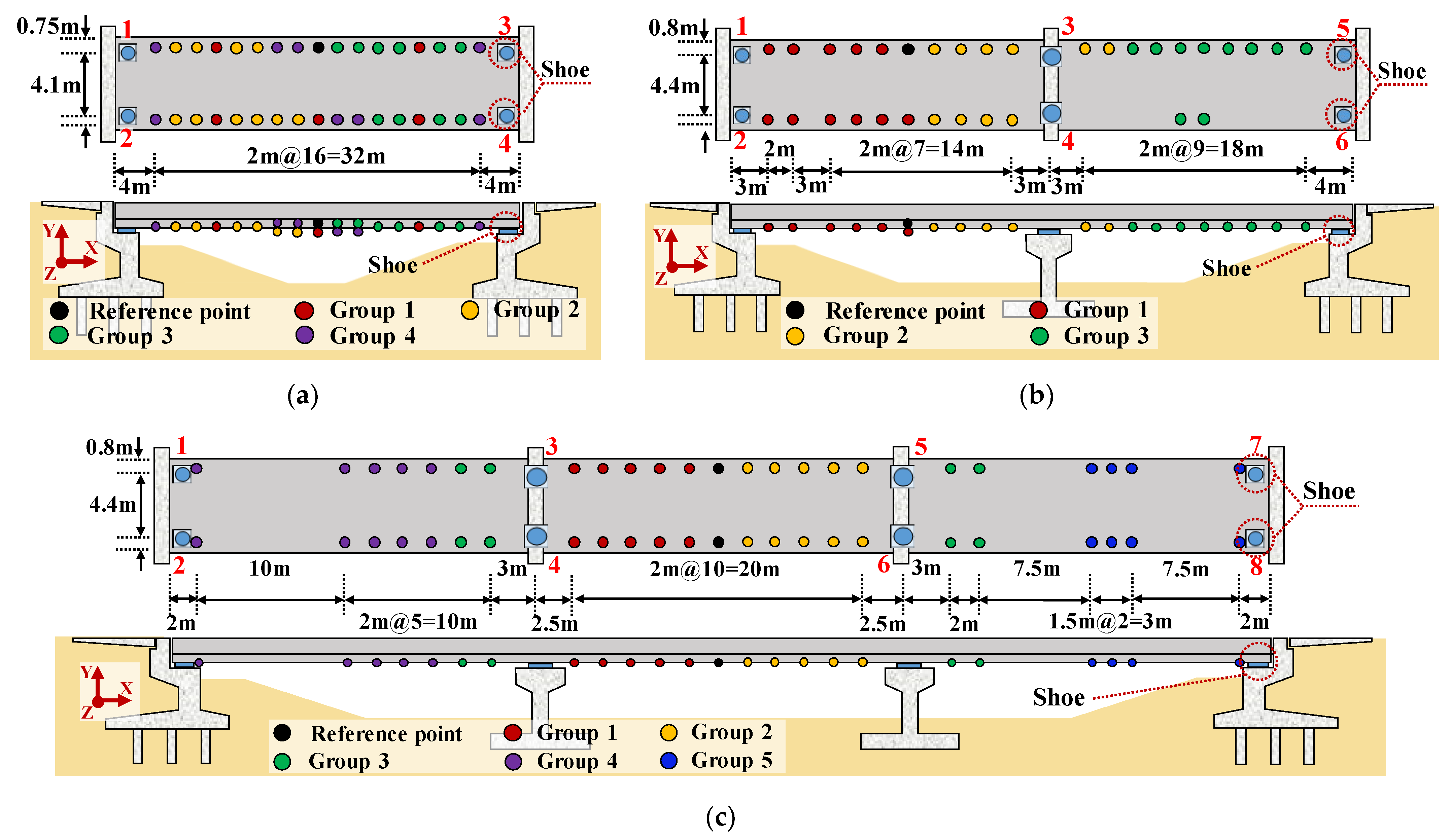
2.2. Experimental Setup

The train speed (approximately 270 km/h to 300 km/h) and load on the bridges that connect Busan, Gyeongju, and Daegu on the Gyeongbu high-speed railway in Korea hardly change. Likewise, the northbound and southbound tracks for high-speed trains do not intersect on the target bridges. Consequently, measurement was taken when high-speed trains passed along the northbound track in order to acquire a response under similar load conditions. Limiting the load characteristics of a bridge according to the operation characteristics of high-speed trains is helpful in examining the numerical model.

In order to estimate the accurate dynamic properties of the high-speed railway bridges in the field, the response measured at various points is required. A wireless measurement system was applied in order to measure the response at various points using a small number of sensors. The wireless measurement system is an excellent tool for measuring at various points because of its mobility. Figure 2 shows the wireless measurement system (NARADA system) used in the ambient vibration test [40,41]. Figure 2a shows the NARADA Wireless Sensing Unit (WSU) and accelerometer installed on the high-speed railway bridges, while Figure 2b shows the laptop on which the base station of the NARADA system was installed.

Ambient vibration was measured in the lower part of each bridge because measuring the response on the tracks in the upper part may affect the operation of the trains. For the response measurement, the acceleration response sensitive to dynamic properties was measured for all frequency bands. This was measured in the lower part of the northbound and southbound tracks of each bridge at regular intervals for an accurate mode shape analysis. The measurement point roaming method was applied in order to acquire the response of each bridge at various points using a small number of sensors. The measurement point roaming method is applicable because the loads applied by high-speed trains are similar for high-speed railway bridges. In addition, it can be an excellent solution for accurate measurement with a limited number of sensors in the field test. Figure 3 shows the measurement positions and groups for the target bridges. All measurement points for the target bridges were classified into three to five groups, while measurement was performed by using up to 11 sensors. Following the measurement, the reference point for signal processing was selected in the lower part of the northbound track in the center of the bridge, and the response of the reference point was continuously measured in each group. Despite the time interval between each group, the correlation between them can be estimated by comparing the signals measured at the reference point. In order to apply the measurement point roaming method, the responses acquired from the reference points among the responses measured from each group are normalized. Other than the responses acquired from the reference point, the remaining responses are normalized using the coefficient values applied to the normalization for each group. For all groups, the normalized signals are not subjected to time synchronization; however, the response magnitude is normalized, and the data can be used to estimate the dynamic properties of the structure. The acceleration response was acquired for 50 s so that the ambient vibration section during and after the travel of a high-speed train could be included. The sampling rate was also set to 200 Hz in order to remove aliasing errors.

Table 2. Boundary conditions of the target bridges.

Constraints	Imgi 2nd Bridge	Maeaji Bridge	Hwalchun Bridge
x, z	1, 3	1, 3, 5	1, 3, 5, 7
x, y, z	2, 4	2, 4, 6	2, 4, 6, 8

shows the boundary conditions of the target bridges shown in Figure 3. Numerical model updating was performed by using the boundary conditions.

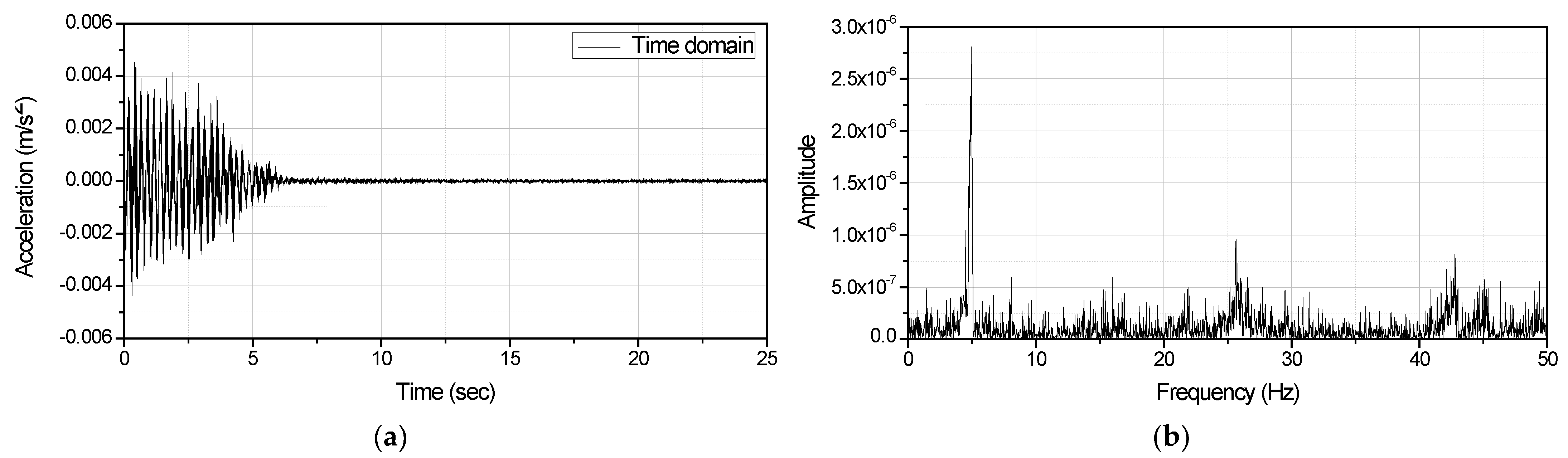
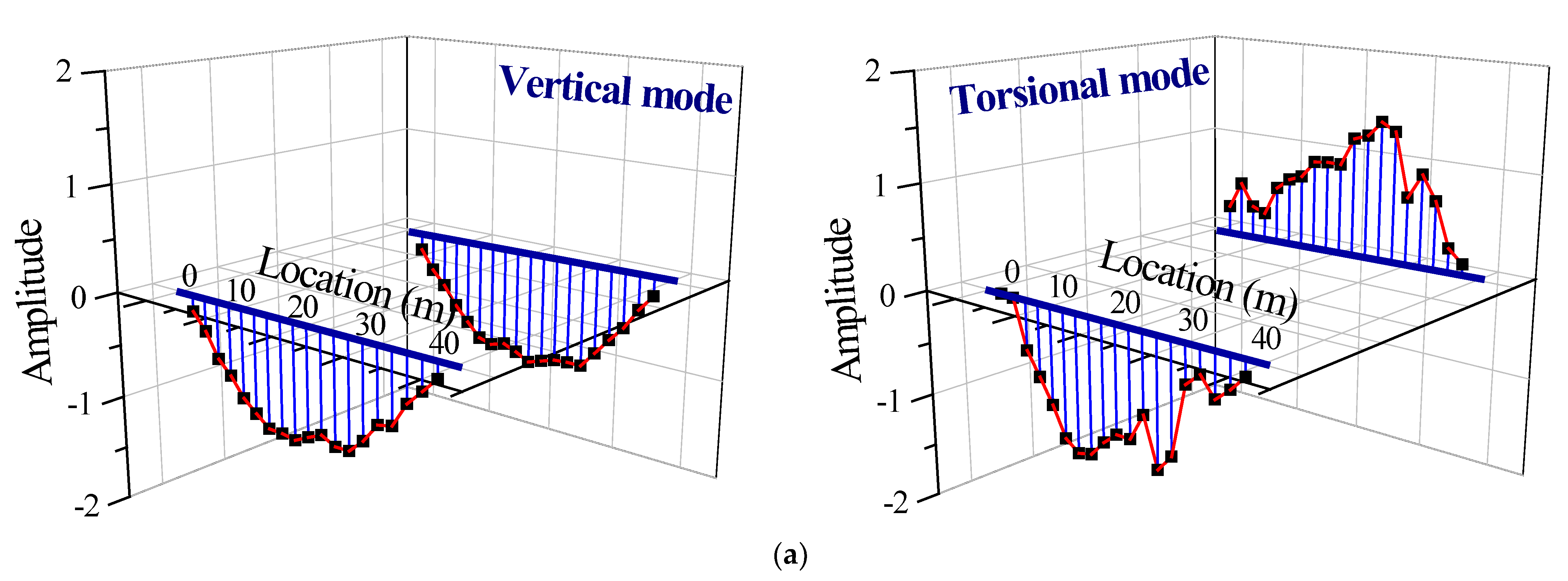
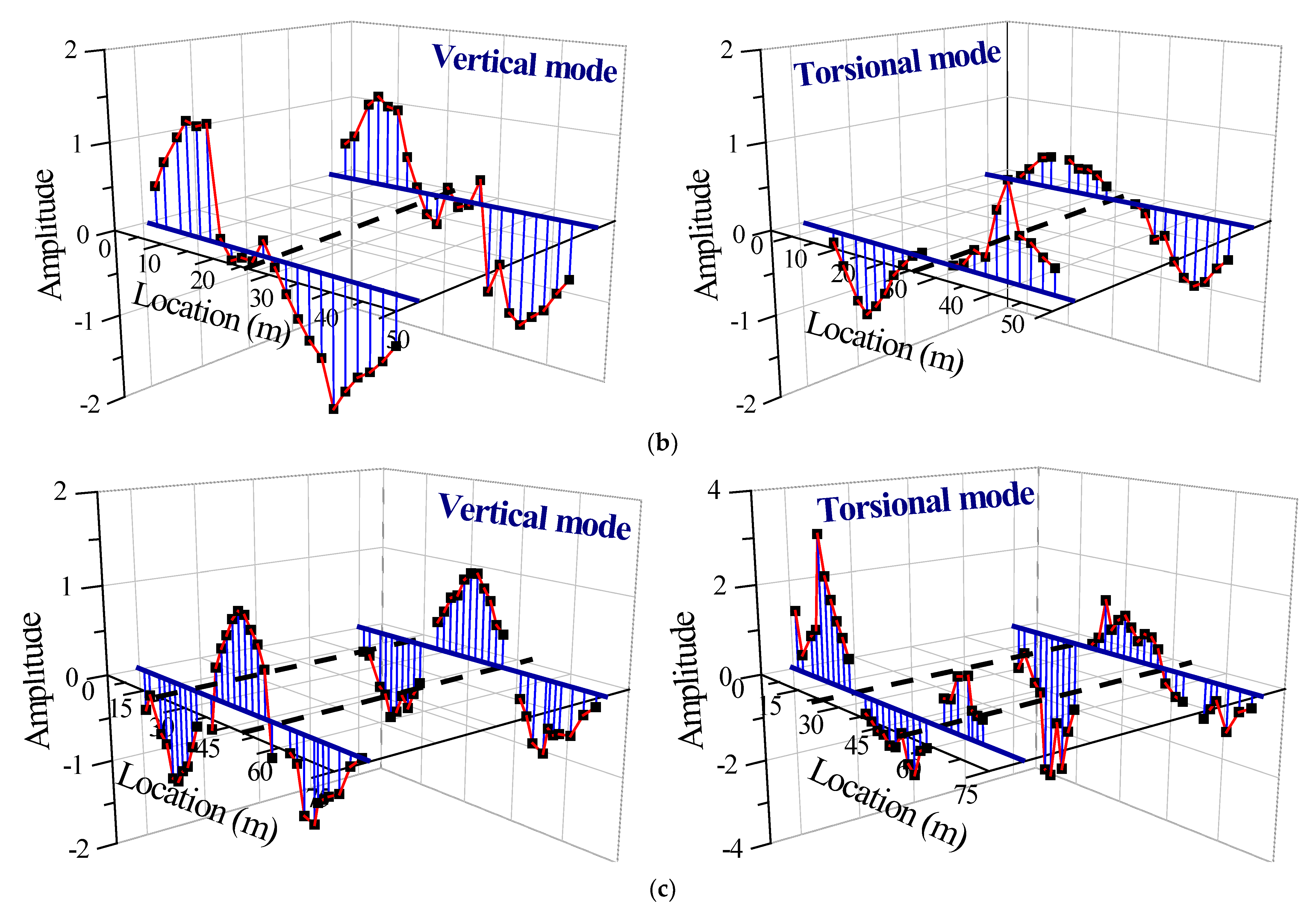
3. Estimation of the Dynamic Properties of the High-Speed Railway Bridges

The cross-correlation function was applied in order to estimate the dynamic properties of the high-speed railway bridges using the response measured from different points in the ambient vibration test [42]. Although the ambient vibration condition is similar whenever a high-speed train passes, the response measured from the bridge is not the same because of the varying load acting on the bridge. Therefore, applying the cross-correlation function in the measurement point roaming method is a useful signal processing method. Cross-correlation function is used for each measurement group in order to determine the same frequency component using the responses measured at different positions of the structure and different times. Cross-correlation signal involves distortion in the time and frequency domains in relation to the original signal. The main characteristics of a signal can be effectively found since such distortion occurs in a direction that further emphasizes parts with high correlations among the components of the two signals. The cross-correlation function can be expressed as Equation (1),

$$R_{xy}\left(\tau \right)=\frac{1}{N}{\displaystyle \sum }_{k=1}^{N}x\left(k\right)y\left(k+\tau \right)$$

(1)

where $x\left(k\right)$ and $y\left(k\right)$ are the $k$-th measured values for the measured signals $x$ and $y$. $N$ is the number of data to be used in the cross-correlation function, and $\tau$ is the time newly defined in the cross-correlation function.

The most common method for estimating the natural frequency of a structure is peak-picking analysis, which involves applying the Fourier transform to the measured response. The natural frequency was estimated in this study by using the response to which the cross-correlation function was applied. In order to exclude the mass effect caused by high-speed trains, natural frequency was estimated by using the response to which the cross-correlation function was applied in the ambient vibration section. The natural frequency to be used for numerical model updating was determined by calculating the average value of the estimated natural frequency values. Figure 4 shows the results of applying the Fourier transform to the response obtained by applying the cross-correlation function to estimate the natural frequency in the Imgi 2nd Bridge.

Extended Kalman filter was used in this study in order to estimate the damping ratio of each high-speed railway bridge [43]. Methods based on the half-power bandwidth and logarithmic decrement, which are commonly used to estimate the damping ratio, cannot be properly applied when the natural frequency of the response measured from a structure changes. However, the estimation of the damping ratio using the extended Kalman filter shows stable damping ratio analysis results compared to the methods based on the half-power bandwidth and logarithmic decrement because the natural frequency of response is estimated along with the damping ratio.

The mode shape of each high-speed railway bridge was estimated by applying proper orthogonal decomposition to the response obtained via the cross-correlation function [44]. Proper orthogonal decomposition, a method of finding a coordinate system to express temporally and spatially ir-regular fluctuation fields, is used to estimate the mode shape of each mode through mode decomposition. If the linear sum of a specific mode in the response of a structure is expressed as Equation (2), the response of the entire structure, $\mathsf{{\rm X}}$, can be expressed as Equation (3).

$$\overrightarrow{x}\left(k,t\right)={\displaystyle \sum }_{r=1}^L{\varphi }_r\left(k\right)q_r\left(t\right)$$

(2)

$$\left[\mathsf{{\rm X}}\right]=\left[\begin{array}{cccc}{x}_1\left(t_1\right)& x_2\left(t_1\right)& \cdots & x_L\left(t_1\right)\\ x_1\left(t_2\right)& x_2\left(t_2\right)& \cdots & x_L\left(t_2\right)\\ ⋮& ⋮& \cdots & ⋮\\ x_1\left(t_{\mathrm{N}}\right)& x_2\left(t_{\mathrm{N}}\right)& \cdots & x_L\left(t_N\right)\end{array}\right]=\left[{\left\{q\right\}}_1{\left\{\varphi \right\}}_1^T+\cdots +{\left\{q\right\}}_L{\left\{\varphi \right\}}_L^T\right]$$

(3)

In Equation (2), $\overrightarrow{x}\left(k,t\right)$ is the vector at time $t$ of the $k$-th mode, ${\varphi }_r\left(k\right)$ is the $r$-th normal mode, $q_r\left(t\right)$ is the $r$. -th eigenvibration vector, and $L$. is the number of modes to be considered. In Equation (3), $x_L\left(t_N\right)$ is the value measured at time $t_N$. at the $L$-th measurement position, ${\left\{q\right\}}_L$ is the time history function $q_L\left(t\right)$ with an array of $N\times 1$, and ${\left\{\varphi \right\}}_L$ is the mode shape at the measurement position of the structure. Among the measurement positions, the final measurement position is the $L$. -th measurement position, and the number of data measured at one point is $N$. If the correlation matrix of the measured response is expressed as Equation (4), Equation (5) can be obtained by multiplying both sides of Equation (4) by the $i$-th mode shape ${\left\{\varphi \right\}}_i$.

$$\left[\mathrm{C}\right]=\frac{1}{N}{\left[\mathrm{X}\right]}^T\left[\mathrm{X}\right]$$

(4)

$$\left[\mathrm{C}\right]{\left\{\varphi \right\}}_i={\mathsf{\lambda }}_i{\left\{\varphi \right\}}_i$$

(5)

The eigenvalue ${\mathsf{\lambda }}_i$ can be expressed as $\left(1/N\right){\left\{q\right\}}_i^T{\left\{q\right\}}_j$ in the mode coordinate system ${\left\{q\right\}}_i$, while ${\mathsf{\lambda }}_i$ and the mode shape ${\left\{\varphi \right\}}_i$ can be calculated by using Equation (5). If proper orthogonal decomposition is applied using the cross-correlation signal, the mode shape can be estimated even for the response in which time synchronization is not performed for each group. Figure 5 shows the mode shape estimated by using the acceleration response measured from the target bridges.

In Figure 4, the first vertical mode of the Imgi 2nd Bridge is very dominant, and the first torsional mode, which is the second mode, can be seen below 50 Hz. Since it is difficult to identify a clear mode after 35 Hz, only dynamic characteristics below 35 Hz were used as target values for numerical model updating.

Table 3. Dynamic properties estimated from the target bridges.

Target Bridge	Mode Type	Natural Frequency (Hz)	Effective Span Length (m)	Damping Ratio (%)
Imgi 2nd Bridge	vertical	4.96	40.75	2.88
	torsional	25.64	37.78	-
Maeaji Bridge	vertical	10.54	25.07	1.66
	torsional	26.29	26.43	-
Hwalchun Bridge	vertical	9.44	23.56	1.93
	torsional	31.36	23.45	-

shows the estimated dynamic properties as target values for numerical model updating. For the mode shape, it is difficult to directly use the response ratio at each position as a target value. As a result, the mode shape was assumed to be the same sine function as the mode shape of the result calculated in the numerical analysis, and half of the period of the sine function was used as the target value. Some of the effective span lengths estimated in Table 3 are longer than the span lengths of the existing bridges. The effective span length is not the actual span length of a bridge; rather, it can be considered as the theoretical value of the length between the intercepts of the mode shape.

4. Dynamic Stability Assessment for High-Speed Railway Bridges

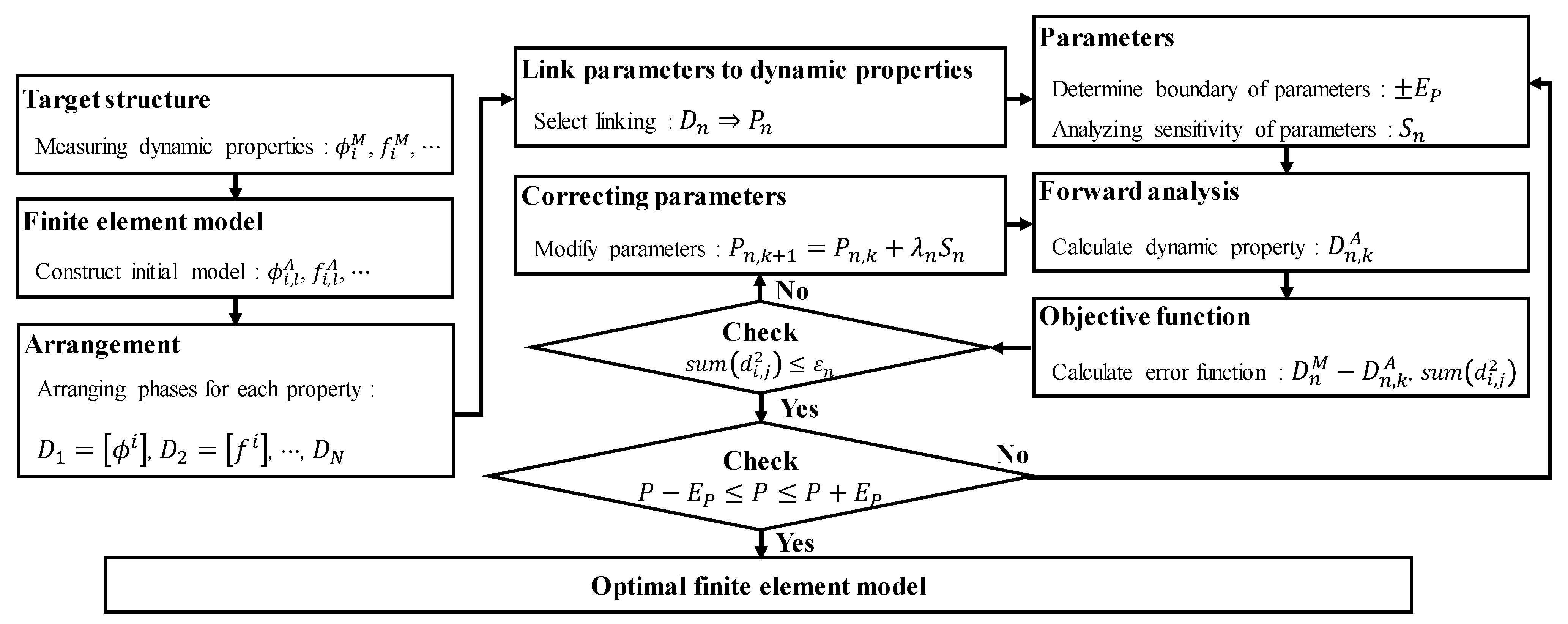
4.1. Algorithm for Numerical Model Updating Using the Univariate Search Method

The univariate search method, one of the unconstrained optimization techniques, is a one-dimensional search method that alters only one variable at a time while fixing the other variables in order to update the approximate value. The univariate search method defines the error function, which is defined as Equation (6), as the object function, and performs optimization in a way that minimizes the error function,

$$\mathrm{Error}=\sqrt{{\displaystyle \sum }_{n=1}^N{\left|{\mathrm{D}}_n^A-{\mathrm{D}}_n^M\right|}^2}$$

(6)

where ${\mathrm{D}}_n^M$ is the $n$-th dynamic property estimated from the measurement and ${\mathrm{D}}_n^A$ is the $n$-th dynamic property calculated by using numerical analysis. If the objective function is set as a simple error function, as shown in Equation (6), the convergence of optimization can be difficult in the presence of many target values because all objective functions cannot be satisfied. Therefore, the objective function was set as the relative error of variables in order to perform numerical model updating using many target values, as shown in Equation (7). Here, ${\mathrm{P}}_{n,k}$ shows variables for the $n$-th dynamic property for the $k$-th calculation.

$$\mathrm{Relative}\mathrm{Error}, d_k=\frac{{\mathrm{P}}_{n,k}-{\mathrm{P}}_{n,k-1}}{{\mathrm{P}}_{n,k}-1}$$

(7)

In order to perform numerical model updating based on the univariate search method, each target value is updated through different variables. The variables can be sequentially updated only if the target values other than the $n$-th variable have extremely low sensitivity for the $n$-th variable when each target value is updated after the target values and variables are set. When the sensitivity of multiple target values to multiple variables is not zero for complex structures such as bridges, the sequential updating of variables will cause errors in the updating results. To prevent such errors, variables were set for each target value, and all the variables were updated using the univariate search method.

The measured value, analyzed value, and mode contribution of the $n$-th dynamic property for numerical model updating can be expressed as Equations (8)–(10),

$${\mathrm{D}}_n^M=\left[d_{n,1}^M, d_{n,2}^M, \cdots ,d_{n,i}^M\right]$$

(8)

$${\mathrm{D}}_{n,k}^A=\left[d_{n,k,1}^A, d_{n,k,2}^A, \cdots ,d_{n,k,i}^A\right]$$

(9)

$${\mathrm{F}}_{k,i}=\left[f_{k,1}, f_{k,2},\cdots ,f_{k,i}\right]$$

(10)

where $d_{n,i}^M$ is the value of the i-th mode of the $n$-th dynamic property measured from the bridge, $d_{n,k,i}^A$ is the value of the $i$-th mode of the $n$-th dynamic property obtained from the $k$-th forward analysis using the numerical model, and $f_{k,i}$ is the mode contribution of the $i$-th mode obtained from the $k$-th forward analysis.

If the variable related to the $n$-th target value ${\mathrm{D}}_n$ in the $k$-th forward analysis of model updating is set as ${\mathrm{P}}_{n,k}$, the variable to be used in the $k+1$-th forward analysis, ${\mathrm{P}}_{n,k+1}$ can be expressed by using the search direction $S_n$ and step distance ${\mathsf{\lambda }}_{n,k}$ of the univariate search method, as shown in Equation (11),

$${\mathrm{P}}_{n,k+1}={\mathrm{P}}_{n,k}\times \left(1+S_n{\mathsf{\lambda }}_{n,k}\right)$$

(11)

where $S_n$ is the search direction determined by the relationship between the $n$-th target value and the variable, and can be expressed as Equation (12). ${\mathsf{\lambda }}_{n,k}$ can be expressed as Equation (13) by using Equations (8)–(10).

$$S_n=\{\begin{array}{ll}1,& \left(d_{n,k,i}^A-d_{n,k-1,i}^A\right)/\left({\mathrm{P}}_{n,k}-{\mathrm{P}}_{n,k-1}\right)\ge 0\\ -1,& \mathrm{Otherwise}\end{array}$$

(12)

$${\mathsf{\lambda }}_{n,k}=1-{\displaystyle \sum }_{i=1}^N{f}_i\cdot d_{n,k,i}^A/d_{n,i}^M/{\displaystyle \sum }_{i=1}^N{f}_i$$

(13)

The variables and target values can be iteratively updated through the forward analysis, and numerical model updating can be completed when the relative error of Equation (7) is equal to or less than the allowable error. The algorithm for numerical model updating based on the univariate search method can be expressed, as shown in Figure 6.

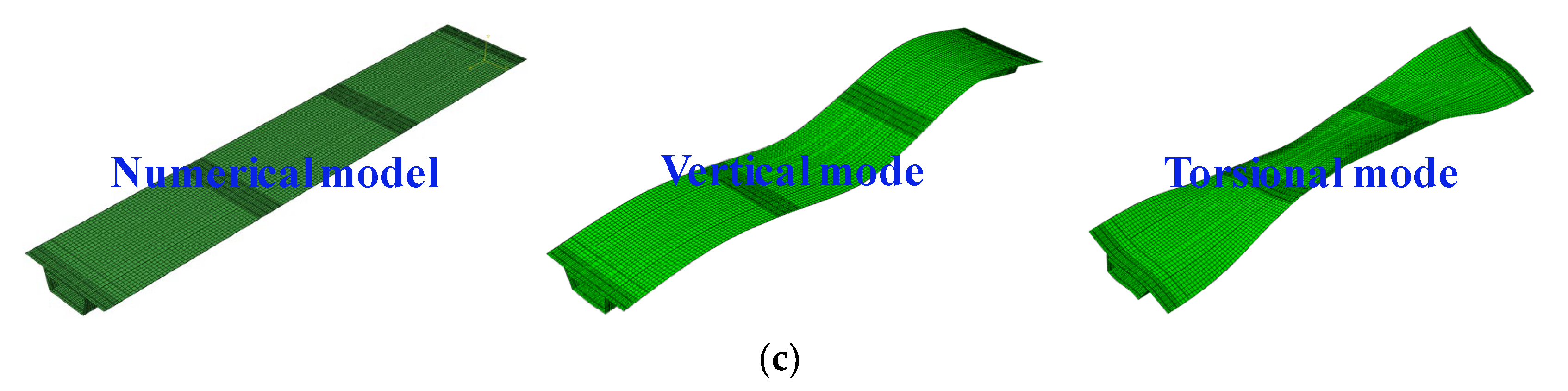
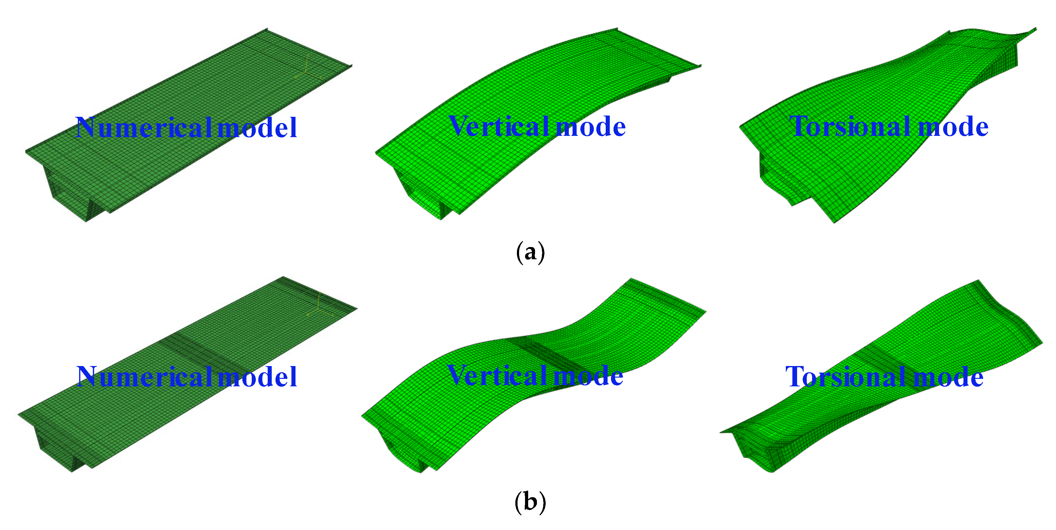
4.2. Numerical Model and Sensitivity Analysis

In this study, numerical model updating was performed by using ABAQUS V6.14, a commercial finite element analysis program, based on the structural design documents of the target bridges. Figure 7 shows the numerical models of the target bridges, which used the shell element, along with the vertical and torsional modes, which are the target values required for numerical model updating.

The natural frequency, effective length, and damping ratio of the main mode are the dynamic properties estimated from the ambient vibration test of the target bridges. Based on the response ratio at each measurement point, the effective length of the mode shape was defined as the distance between two points with zero vertical displacement when the mode shape was assumed to be a sine wave. Consequently, variables associated with these dynamic properties must be set. Variables were limited to the elastic modulus and the distance between the bridge supports because the cross section of each bridge presented in the structural design documents cannot be changed. The distance between the supports can be replaced with the rotational stiffness of the supports. However, the position of the supports must be arbitrarily assumed in order to use the rotational stiffness as a variable. Therefore, supports were assumed to be hinges and the distance between the supports was used as a variable in this study.

Table 4. Sensitivity analysis results for the numerical model of the Imgi 2nd Bridge.

Support Length (m)	Effective Length of Mode Shape (m)		Natural Frequency (Hz)		Elastic Modulus of Concrete (GPa)	Effective Length of Mode Shape (m)		Natural Frequency (Hz)
	Vertical (4.96 Hz)	Torsional (25.64 Hz)	Vertical (4.96 Hz)	Torsional (25.64 Hz)		Vertical (4.96 Hz)	Torsional (25.64 Hz)	Vertical (4.96 Hz)	Torsiona (25.64 Hz)
40	42.985	40.995	4.314	19.686	40	39.775	38.587	4.918	20.273
39.2	40.846	39.343	4.625	19.844	42	39.773	38.583	5.033	20.726
38.4	39.776	38.590	4.829	19.927	44	39.772	38.580	5.145	21.169
37.6	38.894	37.984	5.019	19.997	46	39.770	38.577	5.255	21.603
36.8	38.066	37.397	5.208	20.068	48	39.769	38.574	5.363	22.028
36	37.268	36.816	5.400	20.138	50	39.768	38.571	5.469	22.445
constant	elastic modulus of concrete: 35 GPa				constant	support length: 38.4 m

shows the sensitivity analysis results of the dynamic properties according to the change in variables for the numerical model of the Imgi 2nd Bridge.

In Table 4, the natural frequency of the Imgi 2nd Bridge is sensitive to both the support length and the elastic modulus of concrete. The effective length of the mode shape is highly sensitive to the support length; however, it exhibits low sensitivity to the elastic modulus of concrete. Therefore, for numerical model updating, the univariate search method was applied by using the support length as a variable for the effective length of the mode shape and the elastic modulus as a variable for the natural frequency.

For precise numerical model updating, many variables need to be set. In the case of numerical model updating based on the univariate search method, the number of variables that can be set is the same as the number of target values that can be determined. As a result, expected changes in variables that cannot be set may appear as changes in variables that are set for numerical model updating. This indicates that the set variables can be considered as representative engineering values rather than physical values.

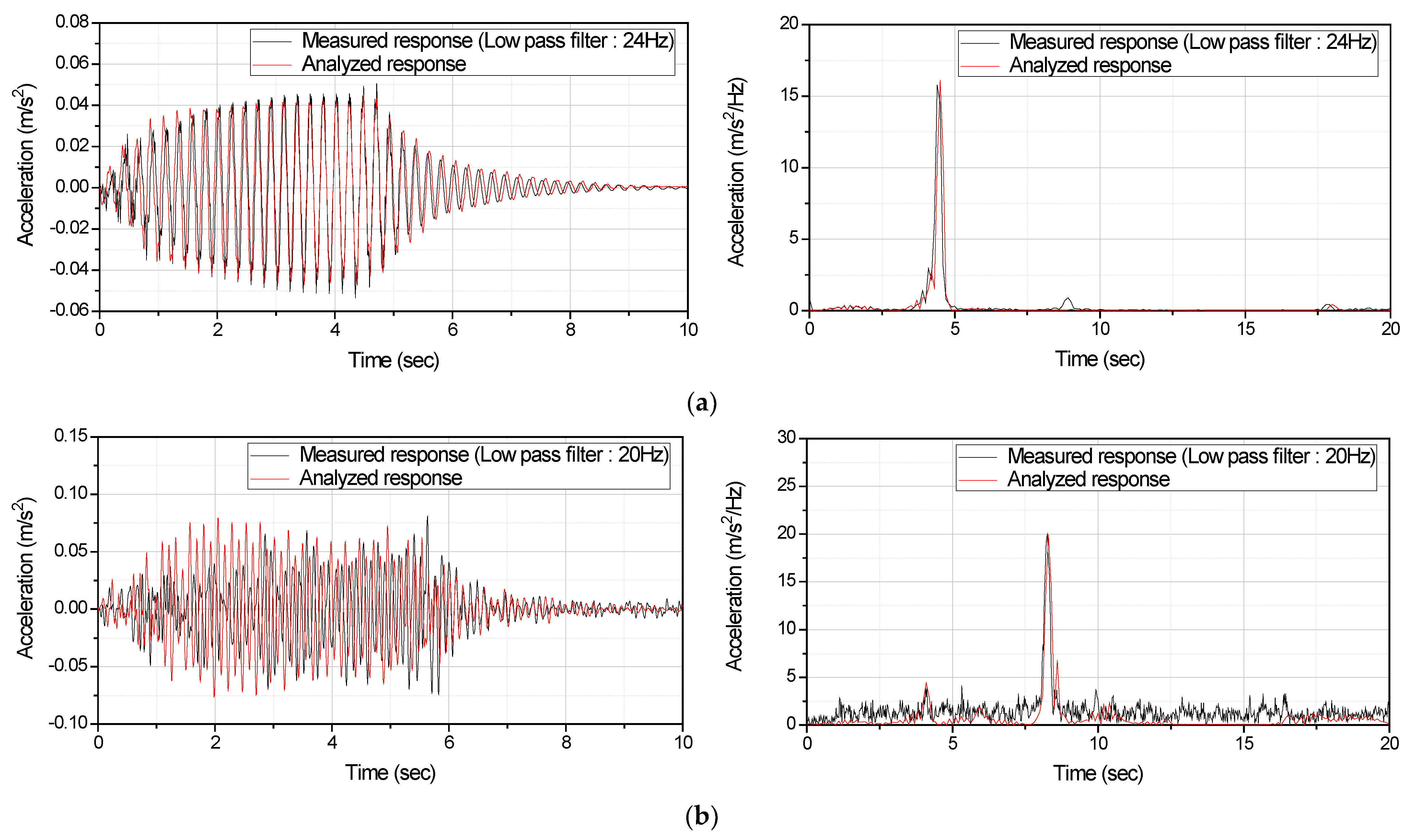
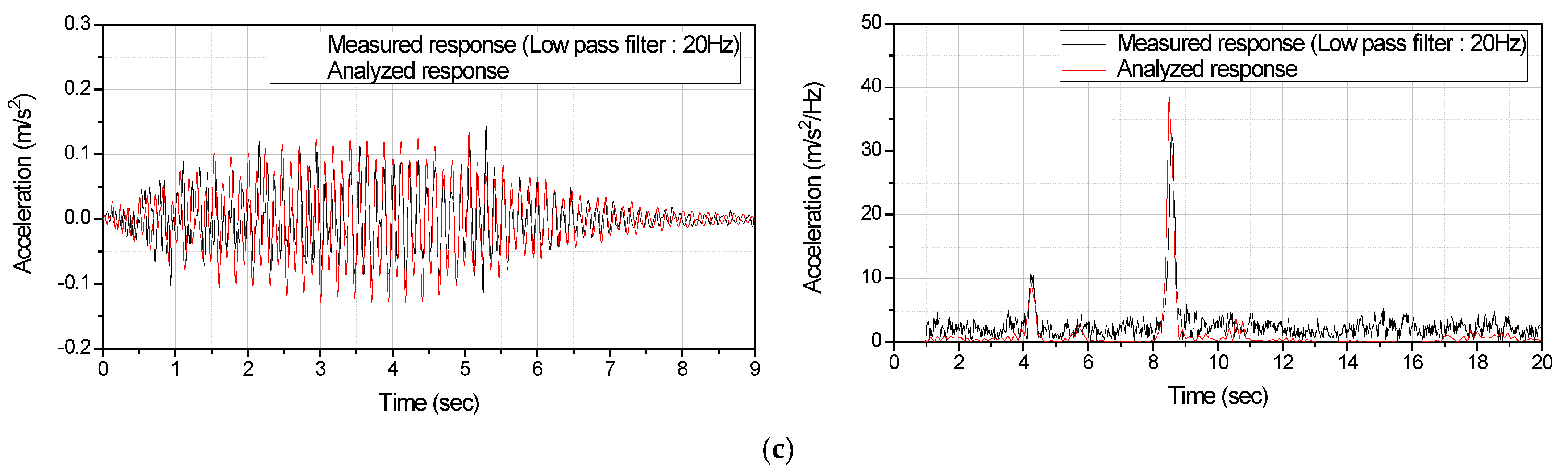
4.3. Numerical Model Updating and Moving Load Analysis

Based on the structural design documents, the elastic modulus and support length are the variables used to update the numerical models. Since concrete has a compressive strength of 40 MPa, the initial value of the elastic modulus was calculated to be 35 GPa. The initial value of the support length was set as the value obtained by subtracting the elastic bearings from the total span length. These initial values do not affect the updated final results even if they are set as arbitrary values because they are used to shorten the numerical analysis updating process.

Table 5. Numerical model updating process of the Imgi 2nd Bridge.

Number of Iteration	Parameter		Dynamic Property
	Support Length (m)	Elastic Modulus (GPa)	Number of Result	Natural Frequency (Hz)		Effective Span Length (m)
				Vertical	Torsional	Vertical	Torsional
			Measured	4.96	25.64	40.75	37.78
initial	38.5	35.00	1	4.32	21.21	39.63	38.29
2	39.4	46.91	2	4.68	24.26	41.17	38.93
3	39.0	52.57	3	5.07	25.63	40.38	38.50
4	39.2	50.55	4	4.93	25.15	40.56	36.68
5	39.4	51.42	5	4.90	25.34	40.98	37.39
6	39.4	52.77	6	4.96	25.65	40.98	37.52

,

Table 6. Numerical model updating process of the Maeaji Bridge.

Number of Iteration	Parameter		Dynamic Property
	Support Length (m)	Elastic Modulus (GPa)	Number of Result	Natural Frequency (Hz)		Effective Span Length (m)
				Vertical	Torsional	Vertical	Torsional
			Measured	10.54	26.29	25.07	26.43
initial	24.2	35.00	1	9.80	26.20	24.73	27.47
2	24.2	39.40	2	10.38	27.78	24.99	28.80
3	24.0	39.40	3	10.49	27.82	24.95	27.70
4	23.8	39.40	4	10.52	27.69	24.79	28.59
5	23.8	38.22	5	10.43	27.48	24.81	29.12

and

Table 7. Numerical model updating process of the Hwalchun Bridge.

Number of Iteration	Parameter		Dynamic Property
	Support Length (m)	Elastic Modulus (GPa)	Number of Result	Natural Frequency (Hz)		Effective Span Length (m)
				Vertical	Torsional	Vertical	Torsional
			Measured	9.44	31.36	23.56	23.45
initial	24.2	35.00	1	7.70	31.74	25.57	29.23
2	23.6	51.79	2	9.54	32.00	24.56	29.66
3	23.6	51.79	3	9.44	31.64	24.39	25.99
4	23.6	43.86	4	9.44	31.64	24.43	26.58

show the process of performing numerical model updating by using the dynamic properties estimated from the ambient vibration test of each target bridge as target values. Numerical model updating was performed until the relative error of Equation (7) was 1% or less. Consequently, the vertical and torsional modes estimated from the measured data differed by less than 5% from those of the updated numerical model.

Since the traveling speeds of high-speed trains differ from each target bridge, each traveling speed must be applied in order to accurately compare the measured and analyzed signals. The traveling speeds of high-speed trains were estimated by using the beating frequency included in the measured acceleration response. The speeds obtained were 300 km/h for the Imgi 2nd Bridge, 275 km/h for the Maeaji Bridge, and 285 km/h for the Hwalchun Bridge. For the moving load analysis, the length, wheel base, and wheel load of a high-speed train passenger car were assumed to be 18.5 m, 15.5 m, and 84,700 kN, respectively. The moving load was applied to the time history analysis of the updated numerical model. It was applied to each node of the rail element over time in the form of a concentrated load, taking into account the speed, wheel base, and wheel load of the high-speed train, and then removed. The damping ratio of 1.66% to 2.88%, which was estimated using the extended Kalman filter in Table 3, was applied to the target bridges.

The frequency to apply the low-pass filter was determined to exclude the influence of the beat frequency by the wheel spacing between each passenger car on the interaction between the high-speed train and the bridge. The train has a 3 m distance between the rear wheels of the front passenger car and the front wheels of the rear passenger car. The corresponding frequency is approximately 27 Hz when the train speed is 300 km/h, and 24 Hz when it is 270 km/h. Therefore, 10% to 15% of the corresponding frequency was applied to the low-pass filter for a comparison between the measured response and the analyzed response in the moving load analysis.

Figure 8 compares the responses measured at the reference point of each target bridge and the responses analyzed using the numerical models in the time and frequency domains. The analyzed responses were slightly larger than the responses measured in the ambient vibration test; however, they were similar when the noise component was excluded. This indicates that numerical model updating was performed well, and that the numerical analysis based on the updated models can replace field testing of high-speed railway bridges.

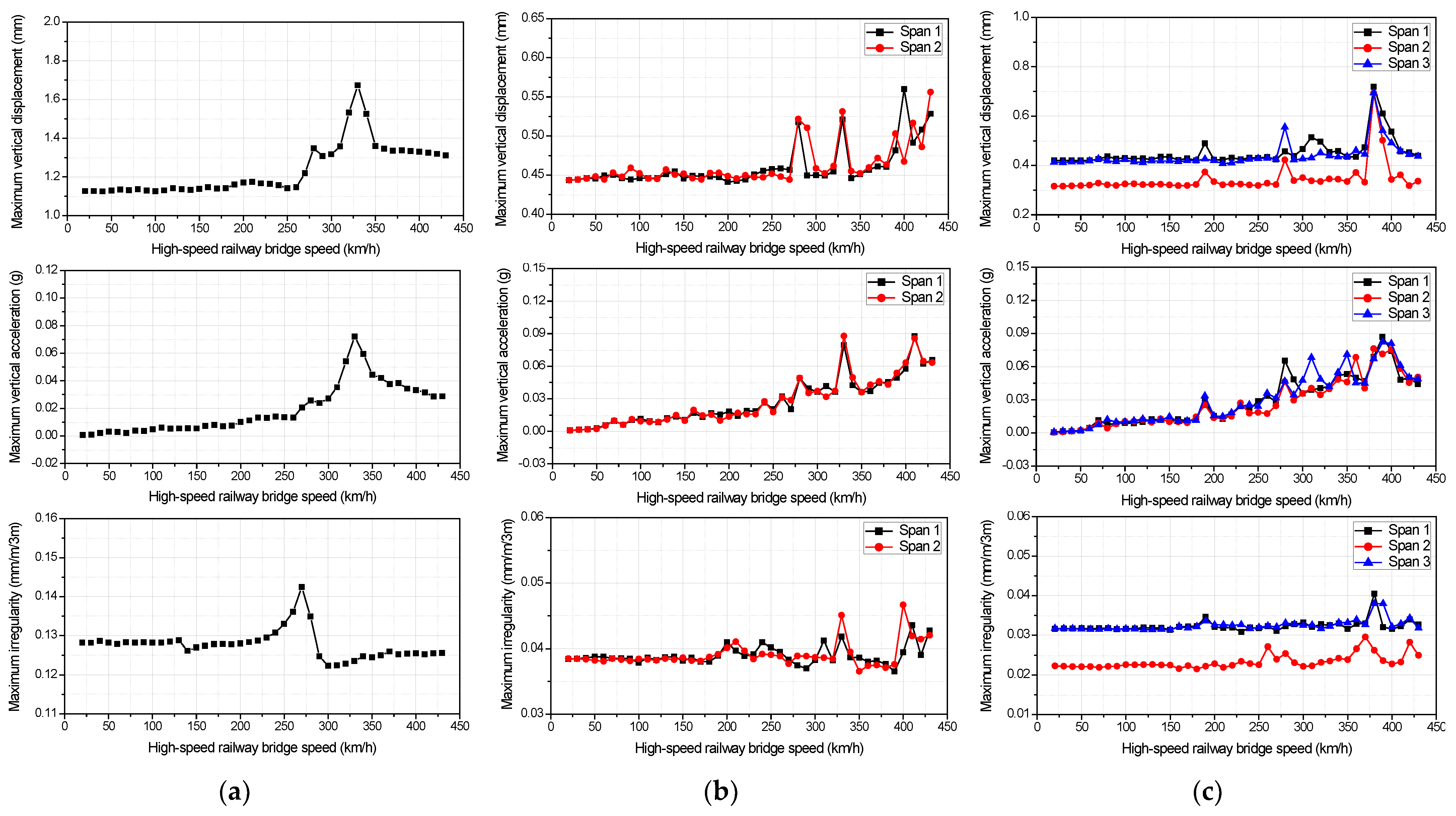
4.4. Dynamic Stability Assessment Using the Updated Numerical Models

The dynamic stability of high-speed railway bridges is necessary in order to determine vibration serviceability and driving stability, and it is required by the high-speed railway design standards of Korea. In this study, dynamic stability assessment was conducted by using the updated numerical models in order to examine the effectiveness of the proposed numerical model updating method and updated numerical models. According to the high-speed railway design standards, dynamic stability is examined up to 1.1 times the design speed with a speed increment of 10 km/h [45]. In this study, however, moving load analysis was conducted for a speed of up to 430 km/h even though the design speed of the target bridges was 350 km/h. In the moving load analysis, the damping ratios estimated using the extended Kalman filter were used, and the speed was increased by 10 km/h in the 20 km/h to 430 km/h range. The maximum vertical displacement of the bridge, maximum vertical acceleration of the upper plate, and maximum vertical ir-regularity of the track according to the train speed were examined in the moving load analysis.

Figure 9 shows the maximum vertical displacement, maximum vertical acceleration of the upper plate, and maximum vertical ir-regularity according to the train speed.

Table 8. Dynamic stability criteria for the target bridges and the results of analysis.

Item	Limit	Maximum Value from Numerical Analysis, (Maximum Velocity)
		Imgi 2nd Bridge	Maeaji Bridge	Hwalchun Bridge
vertical displacement (mm)	3.33	1.67 (330 km/h)	0.56 (400 km/h)	0.72 (380 km/h)
vertical acceleration on top surface (g)	0.5	0.07 (330 km/h)	0.09 (330 km/h)	0.08 (390 km/h)
vertical ir-regularity in track (mm/m/3 m)	1.2	0.14 (270 km/h)	0.05 (400 km/h)	0.04 (270 km/h)

compares the maximum values calculated in the moving load analysis with the dynamic stability criteria presented in the high-speed railway design standards. As shown in the table, all of the target bridges satisfied the high-speed railway design standards. The target bridges also satisfied the dynamic stability criteria even at a train speed of 400 km/h or higher. However, these are the results of the moving load analysis, and the interaction between the high-speed trains and the bridges was not considered.

5. Conclusions

In this study, numerical model updating was performed based on the univariate search method for prestressed concrete (PSC) box girder bridges in operation. The applicability of the numerical model updating method was examined by comparing the updated numerical models with the responses in the time and frequency domains measured from high-speed railway bridges. The usability of the updated numerical models was examined by conducting a dynamic stability assessment of the high-speed railway bridges in operation.

In the field, an ambient vibration test was conducted by using a limited number of wireless sensors, and the measurement point roaming method was applied in order to measure the acceleration response at various points. The load conditions of high-speed railway bridges hardly changed due to the characteristics of high-speed trains. Therefore, responses at various points could be measured in the ambient vibration test of the high-speed railway bridges by using a limited number of sensors based on the measurement point roaming method, and the dynamic properties of the bridges could be estimated.

The conclusions that can be obtained through the application of the proposed numerical model updating method for high-speed railway bridges are as follows:

–

It was confirmed that the method of updating the numerical model based on the iterative univariate search method enables numerical model updating through a small number of iterations without preparing separate differential functions.

–

The results of the moving load analysis that used the updated numerical model could obtain a response similar to the response in the time and frequency domains measured from high-speed railway bridges.

–

The results of the moving load analysis that used the updated numerical model showed that the field test of high-speed railway bridges can be replaced with numerical analysis.

–

It was confirmed that using the updated numerical model allows for the dynamic stability assessment of high-speed railway bridges.

–

It was found that the results of the field tests for high-speed railway bridges, which are difficult to conduct due to economic and physical limitations, can be predicted by using the proposed numerical model updating method.

In this study, the applicability of the proposed numerical model updating method for various types of bridges needs to be further examined, as it was only examined for PSC box girder bridges. Furthermore, if further research on train–bridge interaction is conducted, the proposed method is expected to be useful in examining the maintenance and driving stability of high-speed railway bridges.

References

1. Shin, J.R.; An, Y.K.; Sohn, H.; Yun, C.B. Vibration reduction of high-speed railway bridges by adding size-adjusted vehicles. Eng. Struct. 2010, 32, 2839–2849. [Google Scholar] [CrossRef]
2. Gao, L.; An, B.; Xin, T.; Wang, J.; Wang, P. Measurement, analysis, and model updating based on the modal parameters of high-speed railway ballastless track. Meas. J. Int. Meas. Confed. 2020, 161, 107891. [Google Scholar] [CrossRef]
3. Song, Y.; Liu, Z.; Ronnquist, A.; Navik, P.; Liu, Z. Contact wire irregularity stochastics and effect on high-speed railway pantograph-catenary interactions. IEEE Trans. Instrum. Meas. 2020, 69, 8196–8206. [Google Scholar] [CrossRef]
4. Neves, S.G.M.; Montenegro, P.A.; Jorge, P.F.M.; Calçada, R.; Azevedo, A.F.M. Modelling and analysis of the dynamic response of a railway viaduct using an accurate and efficient algorithm. Eng. Struct. 2021, 226, 111308. [Google Scholar] [CrossRef]
5. Shahbaznia, M.; Mirzaee, A.; Raissi Dehkordi, M. A new model updating procedure for reliability-based damage and load identification of railway bridges. KSCE J. Civ. Eng. 2020, 24, 890–901. [Google Scholar] [CrossRef]
6. He, L.; Reynders, E.; García-Palacios, J.H.; Marano, G.C.; Briseghella, B.; De Roeck, G. Wireless-based identification and model updating of a skewed highway bridge for structural health monitoring. Appl. Sci. 2020, 10, 2347. [Google Scholar] [CrossRef] [Green Version]
7. Zhan, J.; Zhang, F.; Siahkouhi, M.; Kong, X.; Xia, H. A damage identification method for connections of adjacent box-beam bridges using vehicle–bridge interaction analysis and model updating. Eng. Struct. 2021, 228, 111551. [Google Scholar] [CrossRef]
8. Chellini, G.; Nardini, L.; Salvatore, W. Dynamical identification and modelling of steel-concrete composite high-speed railway bridges. Struct. Infrastruct. Eng. 2011, 7, 823–841. [Google Scholar] [CrossRef]
9. Luo, K.; Lei, X.; Zhang, X. Vibration prediction of box girder bridges used in high-speed railways based on model test. Int. J. Struct. Stab. Dyn. 2020, 20, 2050064. [Google Scholar] [CrossRef]
10. Tian, Y.; Zhang, N.; Xia, H. Temperature effect on service performance of high-speed railway concrete bridges. Adv. Struct. Eng. 2017, 20, 865–883. [Google Scholar] [CrossRef]
11. Xiao, X.; Shen, W.; He, X. Track irregularity monitoring on high-speed railway viaducts: A novel algorithm with unknown input condensation. J. Eng. Mech. 2021, 147, 04021029. [Google Scholar] [CrossRef]
12. Vagnoli, M.; Remenyte-Prescott, R.; Andrews, J. Railway bridge structural health monitoring and fault detection: State-of-the-art methods and future challenges. Struct. Health Monit. 2018, 17, 971–1007. [Google Scholar] [CrossRef]
13. Marques, F.; Cunha, Á.; Fernandes, A.A.; Caetano, E.; Magalhães, F. Evaluation of dynamic effects and fatigue assessment of a metallic railway bridge. Struct. Infrastruct. Eng. 2010, 6, 635–646. [Google Scholar] [CrossRef]
14. Gonzales, I.; Ülker-Kaustell, M.; Karoumi, R. Seasonal effects on the stiffness properties of a ballasted railway bridge. Eng. Struct. 2013, 57, 63–72. [Google Scholar] [CrossRef]
15. Zhao, H.W.; Ding, Y.L.; Nagarajaiah, S.; Li, A.Q. Behavior analysis and early warning of girder deflections of a steel-truss arch railway bridge under the effects of temperature and trains: Case study. J. Bridge Eng. 2019, 24, 05018013. [Google Scholar] [CrossRef]
16. Baruch, M.; Itzhack, I.Y.B. Optimal weighted orthogonalization of measured modes. AIAA J. 1978, 16, 346–351. [Google Scholar] [CrossRef]
17. Berman, A.; Nagy, E.J. Improvement of a large analytical model using test data. AIAA J. 1983, 21, 1168–1173. [Google Scholar] [CrossRef]
18. Wei, F.H. Mass and stiffness interaction effects in analytical model modification. AIAA J. 1990, 28, 1686–1688. [Google Scholar] [CrossRef]
19. Mulvey, J.M.; Ruszczyński, A. A new scenario decomposition method for large-scale stochastic optimization. Oper. Res. 1995, 43, 477–490. [Google Scholar] [CrossRef]
20. Ross, R.G., Jr. Synthesis of stiffness and mass matrices from experimental vibration modes. SAE Tech. Pap. 1971, 80, 710787. [Google Scholar]
21. Thoren, A. Derivation of mass and stiffness matrices from dynamic test data. In Proceedings of the 13th Structures, Structural Dynamics, and Materials Conference, San Antonio, TX, USA, 10–12 April 1972; p. 346. [Google Scholar]
22. Caesar, B. Updating system matrices using modal test data. In Proceedings of the 5th International Modal Analysis Conference, London, UK, 6–9 April 1987; pp. 453–459. [Google Scholar]
23. Link, M.; Weiland, M.; Barragan, J.M. Direct physical matrix identification as compared to phase resonance testing: Assessment based on practical application. In Proceedings of the 5th International Modal Analysis Conference, London, UK, 6–9 April 1987; pp. 804–811. [Google Scholar]
24. Sidhu, J.; Ewins, D.J. Correlation of finite element and modal test studies of a practical structure. In Proceedings of the 2nd International Modal Analysis Conference & Exhibit, Orlando, FL, USA; pp. 756–762.
25. Gysin, H.P. Critical application of an error matrix method for location of finite element modeling inaccuracies. In Proceedings of the 4th International Modal Analysis Conference, Los Angeles, CA, USA, 3–6 February 1986; Volume 2, pp. 1339–1351. [Google Scholar]
26. Lieven, N.A.J.; Ewins, D.J. Expansion of modal data for correlation. In Proceedings of the 8th International Modal Analysis Conference, Orlando, FL, USA, 29 January–1 February 1990; pp. 605–609. [Google Scholar]
27. Mottershead, J.E.; Friswell, M.I. Model updating in structural dynamics: A survey. J. Sound Vib. 1993, 167, 347–375. [Google Scholar] [CrossRef]
28. Maia, N.M.M.; Silva, J.M.M. Theoretical and Experimental Modal Analysis; Research Studies Press: Hertfordshire, UK, 1997. [Google Scholar]
29. Levin, R.I.; Lieven, N.A.J. Dynamic finite element model updating using neural networks. J. Sound Vib. 1998, 210, 593–607. [Google Scholar] [CrossRef]
30. Thonon, C.; Golinval, J.C. Results obtained by minimizing natural frequency and mac-value errors of a beam model. Mech. Syst. Signal Process. 2003, 17, 65–72. [Google Scholar] [CrossRef]
31. Jaishi, B.; Ren, W.X. Structural finite element model updating using ambient vibration test results. J. Struct. Eng. 2005, 131, 617–628. [Google Scholar] [CrossRef]
32. Feng, D.; Feng, M.Q. Model updating of railway bridge using in situ dynamic displacement measurement under trainloads. J. Bridge Eng. 2015, 20, 04015019. [Google Scholar] [CrossRef]
33. Jung, D.S.; Kim, C.Y. Finite element model updating on small-scale bridge model using the hybrid genetic algorithm. Struct. Infrastruct. Eng. 2013, 9, 481–495. [Google Scholar] [CrossRef]
34. Holland, J.H. Adaptation in Natural and Artificial Systems; University of Michigan Press: Ann Arbor, MI, USA, 1975. [Google Scholar]
35. Levin, R.I.; Lieven, N.A.J. Dynamic finite element model updating using simulated annealing and genetic algorithms. Mech. Syst. Signal Process. 1998, 12, 91–120. [Google Scholar] [CrossRef] [Green Version]
36. Modak, S.V.; Kundra, T.K.; Nakra, B.C. Model updating using constrained optimization. Mech. Res. Commun. 2000, 27, 543–551. [Google Scholar] [CrossRef]
37. Jaishi, B.; Ren, W.X. Damage detection by finite element model updating using modal flexibility residual. J. Struct. Eng. 2006, 290, 369–387. [Google Scholar] [CrossRef]
38. Ribeiro, D.; Calçada, R.; Delgado, R.; Brehm, M.; Zabel, V. Finite element model updating of a bowstring-arch railway bridge based on experimental modal parameters. Eng. Struct. 2012, 40, 413–435. [Google Scholar] [CrossRef]
39. Rao, S.S. Engineering Optimization: Theory and Practice, 3rd ed.; John Wiley & Sons: New York, NY, USA, 1996; p. 903. [Google Scholar]
40. Lynch, J.P.; Law, K.H.; Kiremidjian, A.S.; Kenny, T.W.; Carryer, E.; Partridge, A. The design of a wireless sensing unit for structural health monitoring. In Proceedings of the 3rd International Workshop on Structural Health Monitoring, Stanford, CA, USA, 12–14 September 2001. [Google Scholar]
41. Wang, Y.; Lynch, J.P.; Law, K.H. Validation of an integrated network system for real-time wireless monitoring of civil structures. In Proceedings of the 5th International Workshop on Structural Health Monitoring, Stanford, CA, USA, 12–14 September 2005. [Google Scholar]
42. Helleseth, T. Some results about the cross-correlation function between two maximal linear sequences. Discret. Math. 1976, 16, 209–232. [Google Scholar] [CrossRef] [Green Version]
43. Park, D.U.; Kim, N.S.; Kim, S.I. Damping estimation of railway bridges using extended Kalman filter. Trans. Korean Soc. Noise Vib. Eng. 2009, 19, 294–300. [Google Scholar]
44. Berkooz, G.; Holmes, P.; Lumley, J.L. The proper orthogonal decomposition in the analysis of turbulent flows. Annu. Rev. Fluid Mech. 1993, 25, 539–575. [Google Scholar] [CrossRef]
45. Korea Rail Network Authority. Design Guideline for Ho-nam High Speed Railway; Korea Rail Network Authority: Daejeon, Korea, 2007. [Google Scholar]
Figure 1. Target bridges: (a) Imgi 2nd Bridge; (b) Maeaji Bridge; (c) Hwalchun Bridge.
Applsci 12 03948 g001
Figure 2. Wireless measurement system: (a) NARADA WSU and accelerometer; (b) Base station and laptop.
Applsci 12 03948 g002
Figure 3. Measurement positions and groups on the target bridges: (a) Imgi 2nd Bridge; (b) Maeaji Bridge; (c) Hwalchun Bridge.
Applsci 12 03948 g003
Figure 4. Cross-correlation signal measured in the Imgi 2nd Bridge: (a) Time domain; (b) Frequency domain.
Applsci 12 03948 g004
Figure 5. The mode shape estimated by applying proper orthogonal decomposition at the target bridges: (a) Imgi 2nd Bridge; (b) Maeaji Bridge; (c) Hwalchun Bridge.
Applsci 12 03948 g005aApplsci 12 03948 g005b
Figure 6. Numerical model updating algorithm based on the univariate search method.
Applsci 12 03948 g006
Figure 7. Numerical models of the target bridges using a commercial finite element analysis program: (a) Imgi 2nd Bridge; (b) Maeaji Bridge; (c) Hwalchun Bridge.
Applsci 12 03948 g007aApplsci 12 03948 g007b
Figure 8. Comparison of the measured and analyzed responses from the target bridges: (a) Imgi 2nd Bridge; (b) Maeaji Bridge; (c) Hwalchun Bridge.
Applsci 12 03948 g008aApplsci 12 03948 g008b
Figure 9. Dynamic stability of the target bridges according to the train speed: (a) Imgi 2nd Bridge; (b) Maeaji Bridge; (c) Hwalchun Bridge.
Applsci 12 03948 g009