Abstract
Hyperspectral remote sensing image classification has been widely employed for numerous applications, such as environmental monitoring, agriculture, and mineralogy. During such classification, the number of training samples in each class often varies significantly. This imbalance in the dataset is often not identified because most classifiers are designed under a balanced dataset assumption, which can distort the minority classes or even treat them as noise. This may lead to biased and inaccurate classification results. This issue can be alleviated by applying preprocessing techniques that enable a uniform distribution of the imbalanced data for further classification. However, it is difficult to add new natural features to a training model by artificial combination of samples by using existing preprocessing techniques. For minority classes with sparse samples, the addition of sufficient natural features can effectively alleviate bias and improve the generalization. For such an imbalanced problem, semi-supervised learning is a creative solution that utilizes the rich natural features of unlabeled data, which can be collected at a low cost in the remote sensing classification. In this paper, we propose a novel semi-supervised learning-based preprocessing solution called NearPseudo. In NearPseudo, pseudo-labels are created by the initialization classifier and added to minority classes with the corresponding unlabeled samples. Simultaneously, to increase reliability and reduce the misclassification cost of pseudo-labels, we created a feedback mechanism based on a consistency check to effectively select the unlabeled data and its pseudo-labels. Experiments were conducted on a state-of-the-art representative hyperspectral dataset to verify the proposed method. The experimental results demonstrate that NearPseudo can achieve better classification accuracy than other common processing methods. Furthermore, it can be flexibly applied to most typical classifiers to improve their classification accuracy. With the intervention of NearPseudo, the accuracy of random forest, k-nearest neighbors, logistic regression, and classification and regression tree increased by 1.8%, 4.0%, 6.4%, and 3.7%, respectively. This study addresses research a gap to solve the imbalanced data-based limitations in hyperspectral image classification.
1. Introduction
Hyperspectral images provides hundreds of continuous narrow spectral bands, which facilitate the discrimination of different surface features [1,2,3,4]. The rich spectral information obtained from hyperspectral remote sensing images has been widely employed in numerous applications, such as environmental monitoring, agriculture, and mineralogy [1,2]. Hyperspectral image classification is essential in applications that focus on assigning class labels to each pixel [2]. The number of selected training samples in each class may be significantly different in some cases. Such a dataset is called an imbalanced dataset [2,5,6]. Conventionally, the rarest classes are named minority classes, and the remaining ones are called majority classes. In remote sensing classification, dataset imbalance is commonly observed during field sampling owing to the uneven distribution of objects with various sizes seen in nature [2,5,7].
Handling an imbalanced dataset frequently encounters degradation of the prediction accuracy or poor accuracy for the minority class, which are called imbalanced problems [5,6]. The lack of capacity of most machine-learning classifiers to handle imbalanced datasets further contributes to these problems. With the rapid development of computer technology, machine-learning classifiers, such as logistic regression (LR) [8] and random forest (RF) [9], have been widely utilized in hyperspectral image classification, and they have exhibited satisfactory classification performance and excellent generalization [10,11]. However, most classifiers are designed under the assumption that the sample sizes of each class are approximately equal. When using imbalanced data, prejudicial and biased classification results may be obtained [5]. Consequently, the minority classes may be distorted or treated as noise. Even if the prediction model achieves a relatively high overall accuracy, the minority classes may remain unknown [12,13,14]. Additionally, some common classifiers in hyperspectral images that use small spectral signatures are also insensitive to the imbalanced data problem [15,16]. Thus, the classification of imbalanced data remains a significant challenge [17].
Several studies have highlighted the imbalanced data problem and its research value [2,5,7]. Most approaches that mitigate imbalanced data problems can be categorized as: preprocessing techniques [18] or modified classifiers [19]. Preprocessing techniques usually alter an imbalanced dataset into balanced distributions before training classifiers, whereas modified classifiers are often associated with a specific algorithm. Preprocessing techniques can be applied to most algorithms and are more flexible. Among the preprocessing techniques, the resampling methods are widely used to compensate for problems arising due to imbalanced data [5]. Resampling methods balance the dataset by adding samples of the minority classes or deleting samples of majority classes [2,3]. Studies have shown that the classification performance on a balanced distribution is better than that of an imbalanced distribution [20].
Resampling methods are typically categorized as: oversampling, undersampling, and hybrid methods [5]. The most popular approach, oversampling, generates new minority class samples to balance the dataset [21]. This involves the random duplication of minority samples, termed as the synthetic minority oversampling technique (SMOTE) [22]. For each minority sample , SMOTE calculates the distances from to each sample and selects the k-nearest neighbor set . Subsequently, artificial samples are generated by , where is a random number. Artificial samples are clearly generated by a linear combination of existing training samples, which may not add new features to the training process. Conversely, the undersampling method randomly eliminates the majority of samples to balance the data. The most common approaches are random undersampling (RUS) and NearMiss [23]. NearMiss selects the majority of samples with the smallest average distance from the minority classes to balance the training data [23]. The main limitation of these methods is the loss of information from the majority classes [24]. Thus, it is difficult to add new natural features to build classifiers by using existing preprocessing techniques. In general, abundance features are required to improve generalization in classification. Minority classes in an imbalanced dataset lack sufficient features for classification owing to sparse samples. This lack of features results in the failure of specific classifications in remote sensing.
For such an imbalanced problem, semi-supervised learning is a creative solution that utilizes the rich natural features in the unlabeled data. In the remote sensing classification, large amounts of unlabeled image data can be obtained through remote sensors at a low cost [10]. However, acquiring a large amount of labeled data is challenging because of the expensive and time-consuming manual labeling process [5]. Particularly in hyperspectral image classification, the categories are often matched to the species level, which increases the difficulty of collecting ground-truth labels. Massive datasets with few labeled samples are commonly used [5]. Therefore, semi-supervised learning, which leverages the rich natural features of unlabeled images to improve the performance of classifiers, has attracted significant attention [25,26]. Commonly used semi-supervised learning methods have made progress on hyperspectral image classification, including the self-learning [27,28], graph-based [29,30], and active learning [31,32,33] methods. Recently, several studies have focused on the application of generative adversarial networks [34,35,36,37,38] and graph convolutional networks [39,40,41] for semi-supervised hyperspectral image classification. In natural images classification, several semi-supervised learning methods aim to find the most representative class-specific samples from both labeled and unlabeled samples. For example, pseudo-label selects the maximum predicted probability class as the true label for unlabeled samples [42]. The -model combines the labeled and unlabeled data by applying consistency regularization [43]. These methods improve the classification performance and prediction ability of the scene classification data. Furthermore, abundant natural information can be extracted from unlabeled samples. However, these semi-supervised methods assume that the labels cover all classes and that each class is relatively balanced. Indeed, only a few studies have attempted to address the imbalanced data problem by using semi-supervised learning [44,45,46]. The key challenge is the effective utilization of the natural features of unlabeled data to improve the classification performance of hyperspectral image classifiers when dealing with imbalanced data. Furthermore, understanding the extraction of effective labels from a minority class is crucial to improving the performance of the classifier.
To address this problem, we propose a novel semi-supervised learning-based solution called NearPseudo. In NearPseudo, an initialization classifier is built based on training data with label, and then creates the corresponding pseudo-labels for unlabeled data. In order to reduce the misclassification cost and improve the quality of the pseudo-labels, the optimal unlabeled samples are selected according to the nearest distance to minority sample and added to unbalanced datasets with the corresponding pseudo-labels. Thus, the unlabeled data can be used for model training, which ensures the automatic extraction of natural features by the classifiers. Simultaneously, we created a feedback mechanism based on a consistency check, which requires that the adding of pseudo-labels to unlabeled data should be consistent with the minority class. It further improves the quality of the pseudo-label. To verify the proposed method, multiple independent experiments were conducted on the publicly available Xiongan hyperspectral dataset. Unlike the smaller datasets commonly used in the hyperspectral image literature, abundant natural unlabeled samples are available in the Xiongan dataset. The Xiongan dataset is a state-of-the-art high-resolution hyperspectral dataset covering a large area. The corresponding labels for the images were accurate to the species levels. The three contributions of this study are summarized as follows.
- We propose a novel preprocessing solution called NearPseudo, to utilize the natural features of unlabeled data to improve the classification of imbalanced data; NearPseudo generates pseudo-labels for unlabeled samples and creates a feedback mechanism based on a consistency check to increase its reliability.
- Compared to other common processing methods in different imbalanced environments, NearPseudo performs better in hyperspectral image classification, especially in the case of an extremely imbalanced dataset. Simultaneously, NearPseudo can effectively improve the accuracy of most minority classes.
- We report the simplicity and universality of NearPseudo. After balancing by NearPseudo, the classification accuracy of most common classifiers, including RF, classification and regression tree (CART), LR, and k-nearest neighbors (kNN), was improved.
2. Proposed Method
We propose an oversampling approach, NearPseudo, in which the minority class is oversampled from unlabeled samples instead of creating samples from the training data. This approach is designed to use a large amount of unlabeled data, which contains rich, useful information. It may be essential to overcome the limitation of a few new features being added to the training process by only combining existing training samples. Our algorithm constantly iterates and oversamples until it obtains a balanced dataset, in which the number of selected training samples in each class is equal. During each loop, new samples from unlabeled data and their manufactured pseudo-labels are added to a single minority class.
The pseudocode for NearPseudo is shown in Algorithm 1. Suppose we have an imbalanced training dataset and an unlabeled dataset . , where is the label corresponding to , m is the number of classes, n is the number of samples, and v is the number of features/bands. , where z is the number of unlabeled samples. During each loop, a subset is randomly extracted from the unlabeled samples , where q is the number of samples in the random subset . Simultaneously, a random sample is taken from with the label . Then, the algorithm computes the distance between and each sample in as follows:
where is the distance between and in . The algorithm then identified a group of k objects in that were closest to . These objects also need to simultaneously undergo a consistency check. In this process, the training dataset , which labels , was utilized to model multi-classifier , as shown in (2). Then, the consistency check model was constructed by using (3). When , passes the conformance check, and vice versa,
When belongs to k objects and also passes the consistency check, is added to the training dataset with the pseudo-label . The algorithm was recirculated until the training sample was balanced.
| Algorithm 1: Pseudocode for selecting samples and generating labels for NearPseudo. |
Require:, imbalance training set with known labels, where v is the number of bands, n is the number of training samples. Require:, unlabeled set, where z is the size of the unlabeled set. Require:q, the number of samples in a random subset. Require:k, the number of the nearest neighbour samples we obtain for each iteration. 1: initialization classifier 2: 3: select a random subset 4: select a random sample in minority classes 5: compute distances between and each sample in , search k closet samples. 6: initialization: 7: 8: select nearest neighbour 9: generate its pseudo-label 10: check the consistency 11: add to formulate a new sample 12: 13: is the balance training dataset 14: |
3. Materials and Experimental Setup
3.1. Datasets
In our study, the Xiongan dataset was used to evaluate and compare the performance of the proposed method with that of other existing methods [47]. Xiongan is located in Matiwan village of the Xiongan New Area in Hebei Province, China. The Xiongan dataset is a state-of-the-art hyperspectral remote sensing image dataset (Figure 1). The Xiongan New Area is the recently developed special economic zone established by the Chinese government in 2017. The area mainly consists of plains with a warm semi-humid continental monsoon climate [48].
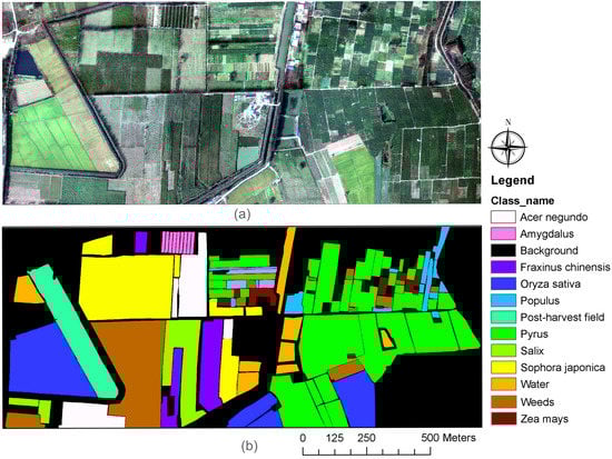
Figure 1.
Hyperspectral remote sensing image and ground truth labels of Xiongan New Area. (a) RGB image and (b) ground truth labels.
The Xiongan dataset was obtained through a flight campaign experiment, which was completed by the Shanghai Institute of Technical Physics (SITP) and the Institute of Remote Sensing Applications (IRSA). SITP and IRSA are both affiliated with the Chinese Academy of Science (CAS). In this flight campaign experiment, data were collected by using an airborne multi-modular imaging spectrometer (AMMIS), which is the latest airborne hyperspectral imaging system developed by SITP [49,50,51]. The AMMIS possesses three modules: visible near-infrared (VNIR), shortwave infrared (SWIR), and long-wave infrared (LWIR). Each module was equipped with three spectrometers and integrated into a hyperspectral imaging system [10]. Based on this system, remote sensing images with high spectral and spatial resolutions can be acquired by using AMMIS.
The hyperspectral images in the Xiongan dataset were collected during the period from 15:40 to 16:03 on 3 October 2017, by using the VNIR module of AMMIS carried by an aircraft. The aircraft was operated at an altitude of 2000 m, with a coverage area of 1320 km. After implementing high-precision geometric correction, band registration, radiometric calibration, and residual strip-noise removal [10,49], 1-level hyperspectral image data with 256 bands and a spectral resolution of 2.4 nm were obtained. As the hyperspectral images were acquired in clear, cloud-free weather conditions, they were less affected by clouds and the atmosphere.
Simultaneously, to manually acquire labels of the Xiongan dataset, IRSA conducted ground-truth investigations and accurately mapped the geometry of each site. In the Matiwan village of Xiongan, the research team investigated 57 sample areas and obtained 39 pictures. Finally, 12 categories were defined based on the ground investigations, as shown in Table 1 and Figure 1. After geographic registration, the ground-truth labels and hyperspectral images constituted a complete Xiongan dataset with a pixel resolution of 3750 × 1580 and spatial resolution of 0.5 m.

Table 1.
Labeled samples of Xiongan.
3.2. Experimental Setup
To evaluate the performance of NearPseudo, three distinct experiments were performed as follows. (1) We performed multiple sampling to generate data subsets with variable degrees of imbalance for comparing the performance of NearPseudo with several other well-known preprocessing methods. The significance of differences between NearPseudo and others was evaluated by the paired t-test. (2) We utilized several types of common hyperspectral image classifiers to classify the unbalanced and balanced datasets and evaluated the performance of NearPseudo. (3) We modulated the different hyperparameters of NearPseudo and performed classification experiments to determine the mechanism for establishing the optimum values of hyperparameters in NearPseudo.
3.2.1. Sampling the Imbalanced Data Subset
In the case of hyperspectral image methods, the processing of imbalanced datasets with varying degrees of imbalance may vary. Thus, to compare the influence of hyperspectral image methods on the classification of datasets with different degrees of imbalance, we designed three training subsets: T1, T2, and T3 (Table 1). R (Max/Min), the ratio of maximum to minimum number of classes, is the difference between the three training subsets, which can be used to measure the degree of imbalance. T1 represents an extremely imbalanced training dataset with R (Max/Min) = 14.0, T2 represents a comparatively imbalanced training dataset with R (Max/Min) = 3.5, and T3 represents a slightly imbalanced training dataset with R (Max/Min) = 1.6 (Table 1). In addition, as shown in Table 1, when designing the three training subsets, we aimed to avoid the repetition of minority classes appearing in the same class. Thus, the results remain unaffected by the data quality of a certain class.
According to the designs in Table 1, we randomly performed multiple sampling to generate imbalanced training and testing datasets on a per-pixel basis without being returned to the dataset. The training and test datasets were two disjoint datasets. In addition, the number of testing data selected for each class was fixed at 2/7 of the number of classes with the maximum training data. As shown in Table 1, we sampled 800 entities from each class equally to construct the testing dataset and avoid the effects of imbalanced data during the testing process.
3.2.2. Processing Method and Classifiers
Following the preprocessing for balancing the data, the dataset was classified by using classifiers. In experiment (1), the classification without processing was compared with classification results from three representative imbalanced processing methods—NearMiss, RUS [23], and SMOTE [22]. These comparison methods are publicly accessible via the imbalance-learn package (https://imbalanced-learn.org/, accessed on 25 August 2017) and are commonly used to compare imbalance processing methods used for hyperspectral image classification [2,3]. Numerous algorithms require manual setting of the hyperparameters. Generally, the range recommended by the algorithm developers is reliable [52]. In our study, most hyperparameters were set to the default values, which were recommended based on experience. In particular, for SMOTE, the number of nearest neighbors was set to 5. For NearMiss, the number of nearest neighbors was 1. RF, as a multi-classifier, was used in NearPseudo. RF is a simple and useful classifier that exhibits excellent performance and better complexity in hyperparameter classification [11,53]. Thus, the RF classifier was used to classify the hyperspectral images for all methods after data was balanced in experiment (1).
Further analysis was conducted to compare the performance and improvement of classifiers after the preprocessing by NearPseudo in experiment (2). The representative classifiers for comparison included RF, CART [54], LR, and kNN [55]. These classifiers are commonly used for multispectral and hyperspectral image classification [10,53] and do not require a large number of labeled datasets to build the model. Similarly, for the above preprocessing methods, these classifiers are publicly accessible through the scikit-learn package (https://scikit-learn.org/, accessed on 1 October 2018) and can be quickly applied for hyperspectral image classification. Numerous papers have detailed the mechanism of these classifiers and have recommended ranges of hyperparameters suitable for remote sensing classification [53,56]. In this study, we adopted these recommended hyperparameter ranges. For RF, the number of trees was set to 180. For kNN, the number of neighbors was set to 11. The other parameters were set to default values. In addition, all experiments were programmed by using Python 3.6 and run on the Ubuntu 14.0 platform with an Intel Xeon e5-2620 CPU and four TITAN XP graphics cards.
3.3. Evaluation Criteria
To assess the accuracy of the hyperspectral image classification, three evaluation metrics are commonly used: (1) overall accuracy (OA), (2) F1-score, and (3) average F1-score (AF) [57]. OA is related to the ratio of correctly classified samples to the total samples, which provides an intuitive interpretation of the accuracy (Equation (5)). In contrast, to evaluate the per-class accuracy, the F1-score of each class was used in our study, which takes into account both recall and precision (Equation (4)) [57]. The F1-score helps to evaluate the accuracy of the majority and minority classes. Additionally, AF, a supplementary accuracy evaluation index, is also listed in our results.
where FN is the false negative, FP is the false positve, TN is the true negative, and TP is the true positive.
4. Results
4.1. Comparison of Classification Results
In this experiment, we compared the accuracy of classification of four preprocessing methods, namely, NearMiss, RUS, SMOTE, and NearPseudo, by recording their respective accuracies before and after processing. We mainly discuss four specific issues: (1) the accuracy of classification of the aforementioned imbalanced preprocessing methods; (2) whether the differences between NearPseudo and others are statistically significant; (3) the enhancement in the accuracy of minority classification after preprocessing, and (4) in the case of training subsets with different degrees of imbalance, whether the different preprocessing methods remain consistent in terms of improving the accuracy. The results are presented in Table 2, Table 3 and Table 4. The final results include the standard deviation values and average of the five experiments.
Table 2.
Classification accuracy (%) of different solutions on sub-training data T1.
Table 3.
Classification accuracy (%) of different solutions on sub-training data T2.
Table 4.
Classification accuracy (%) of different solutions on sub-training data T3.
Table 2 lists the classification results of the different methods on training subset T1, which is an extremely imbalanced training subset with R (Max/Min) = 14.0 (Table 1). We can observe that the performance and accuracy of the classifier increased after preprocessing. The highest AF and OA were achieved by NearPseudo (AF = 74.8 ± 0.3% and OA = 74.8 ± 0.1%), followed by SMOTE (AF = 72.7 ± 0.4% and OA = 72.7 ± 0.2%), RUS (AF = 65.6 ± 0.5% and OA = 65.8 ± 0.1%), and NearMiss (AF = 29.6 ± 0.6% and OA = 32.9 ± 0.2%). Compared with the unbalanced data, NearPseudo improved both AF and OA by 2.5%, respectively, whereas SMOTE improved both AF and OA by 0.4%. The RUS and NearMiss method exhibited low classification performance. The significant result from the paired t-test shows that the AF of NearPseudo was significantly higher than that of NearMiss by 45.2% , significantly higher than that of RUS by 9.2% , and higher than that of SMOTE by 2.1% . As shown in Table 2, after preprocessing by NearPseudo, the F1 scores of nine classes (75%) were improved by varying degrees. Only three classes (25%) obtained the highest F1 value when SMOTE was used to balance the training data, whereas the F1 values of NearMiss and RUS for each species decreased. Notably, the F1 of (NO. 10), which is a minority class with 800 training samples, increased by nearly 13.2% after preprocessing through NearPseudo. Moreover, NearPseudo exhibited outstanding performance on (NO. 3) and (NO. 6), which are minority classes and consist of only 200 training samples. The F1 scores of and improved by approximately 2.0% and 3.1%, respectively.
Table 3 presents the classification results of different balanced methods on the sub-training set T2, with R (Max/Min) = 3.5 (Table 1), which is a relatively imbalanced training subset. These results are similar to those in Table 2. It can be observed that the performance and accuracy of the classifier increased after preprocessing. The best classification performance was achieved after processing by NearPseudo (AF = 75.0 ± 0.4% and OA = 75.1 ± 0.1%), followed by SMOTE (AF = 73.2 ± 0.4% and OA = 73.1 ± 0.2%), RUS (AF = 72.8 ± 0.4% and OA = 72.9 ± 0.2%), and NearMiss (AF = 60.9 ± 0.5% and OA = 60.9 ± 0.1%). Compared to the imbalanced dataset, the classification accuracy was improved by 1.8% after being balanced by NearPseudo. The significant result from the paired t-test shows that the AF of NearPseudo was extremely significantly higher than that of NearMiss by 14.1% , significantly higher than that of RUS by 2.2% , and significantly higher than that of SMOTE by 1.8% . In addition, the F1 score of the 10 classes was improved by 83.33%, and the best accuracy was achieved by NearPseudo. Similarly, the accuracy of these minority classes can be improved by using NearPseudo to various degrees. For example, it can be observed in Table 3 that the classifier exhibited outstanding performance on the (NO. 12) and (NO. 8) classes. These two classes are minority classes and have the fewest samples (only 800 training samples). The F1 score of improved by 6.9%, which is the greatest improvement compared with the other classes. Furthermore, the F1 score of improved by 2.4%.
Table 4 presents the classification results on sub-training set T3, with R (Max/Min) = 1.6 (Table 1). The results are similar to those in Table 2 and Table 3. They show that the best classification performance was achieved by NearPseudo (AF = 76.3 ± 0.4% and OA = 76.5 ± 0.1%), followed by RUS (AF = 76.1 ± 0.4% and OA = 76.2 ± 0.2%), SMOTE (AF = 75.7 ± 0.4% and OA = 76.0 ± 0.2%), and NearMiss (AF = 72.5 ± 0.4% and OA = 72.5 ± 0.1%). Compared to the imbalanced dataset, the classification accuracy improved by 0.4% after being balanced by NearPseudo. The significant result from the paired t-test shows that the AF of NearPseudo was extremely significantly higher than that of NearMiss by 3.8% and significantly higher than that of SMOTE by 0.6% . The difference was not significant between the AF of NearPseudo and that of RUS . The F1 score of 9 classes (75%) improved, and the best performance was exhibited by NearPseudo. It can be observed from Table 4 that the F1 score of three minority classes, (NO. 4), (NO. 9), and (NO. 12), increased by 1.9%, 0.7%, and 0.3%, respectively, thereby verifying the performance of NearPseudo.
Figure 2 depicts the discrepancy in the accuracy of the preprocessing methods in the case of training subsets with different degrees of imbalance. After balancing with NearPseudo, the accuracies of the extremely imbalanced sub-training set T1, relatively imbalanced sub-training set T2, and slightly imbalanced sub-training set T3 improved by 2.6%, 1.9%, and 0.4%, respectively. However, after balancing with SMOTE, the accuracies of T1, T2, and T3 improved by 0.4%, −0.2%, and −0.1%, respectively. With an increase in the degree of imbalance of the dataset, the classification accuracy of the two processing methods increased. This change was most prominent in the case of NearPseudo. The results indicate that the greater the imbalance in the sub-training data, the higher the improvement in the accuracy of the imbalanced data after being balanced by NearPseudo.
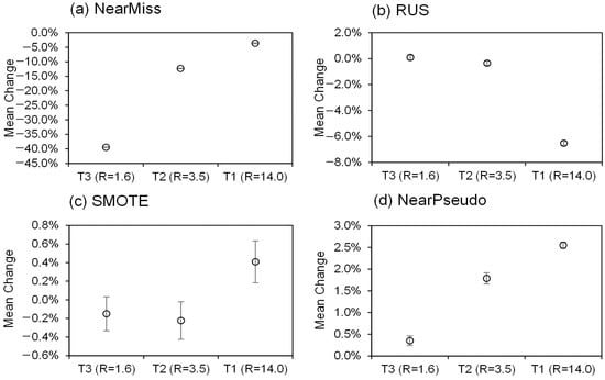
Figure 2.
Mean change in overall accuracy from baseline (unbalanced dataset) to balanced dataset after processing on the three sub-training sets. T1, T2, and T3 represent datasets with different degrees of imbalance. T1 represents an extremely imbalanced training dataset with R (Max/Min) = 14.0, T2 represents a relatively imbalanced training dataset with R (Max/Min) = 3.5, and T3 represents a slightly imbalanced training dataset with R (Max/Min) = 1.6. All data are mean ± standard error from five measurements.
Table 2, Table 3 and Table 4 show that the accuracy of most minority classes can be improved by NearPseudo. In sub-training set T1, the average accuracy of minority classes with minimum sample size (NO. 3 and NO. 6) was improved by 2.6%. In sub-training set T2, the average accuracy of minority classes with minimum sample size (NO. 8 and NO. 12) was improved by 4.7%. In sub-training set T3, the average accuracy of minority classes with minimum sample size (NO. 4, NO. 9, and NO. 12) was improved by 1.0%.
4.2. Comparison of Different Multi-Classification Algorithms
NearPseudo is a preprocessing technique that can improve the capacity of most machine-learning classifiers to handle imbalanced data. As described in the previous subsections, RF was used as the main classifier in NearPseudo. In this experiment, we utilized several types of common classifiers in the hyperspectral images to classify the unbalanced and balanced dataset after preprocessing by NearPseudo. These classifiers included RF, CART, LR, and kNN. Based on the results of classification accuracy (Table 5), we quantitatively evaluated the improvement in the imbalanced ability of these classifiers after the processing of NearPseudo. For this experiment, we illustrate our results by using a detailed example of the imbalanced dataset T2.
Table 5.
Classification accuracy (%) of different solution.
As shown in Table 5, before preprocessing, the RF classifier exhibited the best classification accuracy (OA = 73.3%), followed by kNN (OA = 65.8%), LR (OA = 63.1%), and CART (OA = 57.0%). After processing by NearPseudo, the best classification accuracy was still achieved by the RF (OA = 75.1%), followed by kNN (OA = 69.8%), LR (OA = 69.5%), and CART (OA = 60.7%). As can be seen, after balancing the imbalanced training set T2 using NearPseudo, the classification performance of the four commonly used multi-classifiers improved. Compared with the unbalanced condition, the OA values of RF, kNN, LR, and CART increased by 1.8%, 4.0%, 6.4%, and 3.7%, respectively. The effect of NearPseudo on accuracy is related to the capacity of machine-learning algorithms to handle imbalanced datasets. The classification performance of most multi-classifiers with imbalanced data can be improved by using NearPseudo.
A significant improvement was observed in F1 scores of minority classes in each classifier before and after processing by NearPseudo. In imbalanced dataset T2, the (NO. 12) and (NO. 8) classes were the minority classes and had the fewest samples (only 800 training samples) (Table 1). The F1 scores of these two classes using four common classifiers improved after processing by NearPseudo. In particular, for (NO. 8), the F1 scores of RF, kNN, LR and CART increased by 2.4%, 11.1%, 20%, and 11.9%, respectively. For (NO. 12), the F1 scores of RF, kNN, LR, and CART increased by 6.9%, 11.1%, 20%, and 11.9%, respectively. This further illustrates the improvement in the accuracy of most minority classes and the reduction of bias of most models by NearPseudo.
4.3. Impact of Different Hyperparameters
NearPseudo has two hyperparameters: number of random subset samples q and the number of nearest neighbor samples obtained for each iteration k. The two hyperparameters were selected manually. In this experiment, for NearPseudo, we adopted different values of q = [5000, 10,000, 15,000, 20,000, 25,000, 30,000] and k = [2, 3, 4, 5, 6, 7, 8] (Figure 3). We set different hyperparameters of NearPseudo and performed classification experiments on training subsets T1, T2, and T3 (Table 1). This helped evaluate the impact of the two hyperparameters on the classification accuracy in NearPseudo and further reveal the mechanism underlying the changes in hyperparameters to guide their manual setting in NearPseudo.
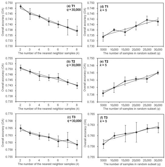
Figure 3.
Impact of two hyperparameters on overall accuracy (OA) in three sub-training sets. (a–c) are representative of the change of OA as the number of the nearest neighbor samples (k) increase in sub-training set T1, T2, and T3, respectively. (d–f) are representative of the change of OA as the number of samples (q) increase in sub-training set T1, T2, and T3, respectively. All data are mean ± standard error from five measurements, and the dashed line shows a linear correlation between OA and each hyperparameters.
All three imbalanced training subsets exhibited a decrease in the OA curve of the classifier with the hyperparameter k of NearPseudo (Figure 3a–c). Specifically, when the parameter k was varied from 2 to 8, the classification OA based on T1 decreased by 1.1% from 74.8% to 73.7% (Figure 3a). Under the same conditions, the classification OA based on T2 decreased by 0.8% from 75.1% to 74.2% (Figure 3b), whereas the classification OA based on T3 decreased by 0.6% from 76.5% to 75.9% (Figure 3c). Thus, it can be deduced that the improvement in the accuracy of the classifier by NearPseudo is affected by the hyperparameter k. The larger the hyperparameter k, the worse the accuracy. The intuitive explanation of this is included in Section 5.2.
In contrast to hyperparameter k, all results of using three imbalanced training subsets showed that the OA curve of the classifier increased with the hyperparameter q (Figure 3d–f). Specifically, when the parameter q was varied from 5000 to 30,000, the classification OA based on T1 increased by 0.7% from 73.4% to 74.1% (Figure 3d). Under the same conditions, the classification OA based on T2 increased by 0.7% from 73.8% to 74.5% (Figure 3e), whereas the classification OA based on T3 increased by 0.4% from 75.8% to 76.2% (Figure 3f). Therefore, improvement in the accuracy of the classifier by NearPseudo is affected by the hyperparameter q; the larger the hyperparameter q, the better the accuracy. The intuitive explanation of this is included in Section 5.2.
5. Discussion
5.1. Effect of NearPseudo on Different Multi-Classification Algorithms
As shown in Table 5, the impacts of NearPseudo on different multi-classification algorithms vary. To reveal the mechanism, Pearson correlation analysis was used to analyze the relationship between two variables: (1) mean change in overall accuracy from baseline unbalanced dataset to balanced dataset after processing in the sub-training set T2 and (2) variance of F1-score for each class before processing. Notably, lower values for variance correlated with better capacity of most machine-learning algorithms to handle imbalanced datasets, and vice versa. For example, the F1-score of minority class (NO. 12) by using classifier LR was 8.0%, which is high variance (variance = 24.7%), whereas the F1 score of minority class (NO. 12) by using classifier RF was 63.2%, which is low variance (variance = 13.64%) (Figure 4 and Table 5). Compared with RF, LR obtained prejudicial and biased classification results in minority, which increased the difference in F1 scores between each class. Consequently, the variance of the F1 score for each class in the LR classifier was larger.
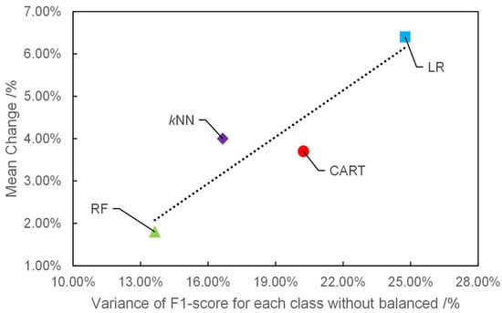
Figure 4.
Mean change in overall accuracy from baseline (unbalanced dataset) to balanced dataset after processing in the sub-training set T2. The dashed line shows a linear correlation between mean change and variance of F1-score for each class without balanced.
As shown in Figure 4, the values of mean change increased as the variance of F1 score for each class without balance. That is, the effect of NearPseudo on accuracy is related to the capacity of most machine-learning algorithms to handle imbalanced datasets. The more negative the impact of the imbalance data on performance of algorithms, the more likely it is that NearPseudo improves the classification accuracy. Conversely, when the algorithm is less affected by imbalanced datasets, there is no additional balanced method required. For the LR classifier, the goal is to find the parameters with optimal values when the minimum value of loss function is obtained. Each class in LR requires sufficient samples to fit the fixed number of parameters. If lacking samples in a minority class, the classifier will perform poorly in this class.
5.2. Effect of Hyperparameters on Performance
In this study, we generated corresponding pseudo-labels for unlabeled data, which allowed us to include unlabeled data in the training process. However, evaluating the accuracy or quality of pseudo-labels is challenging. Existing models to build pseudo-labels have a certain probability of generating false labels. If the samples have false labels or are located in the edge areas to supplement the imbalanced dataset, the classifiers can easily adopt a bias. Therefore, we introduced the nearest neighbor method and a consistency check in NearPseudo to evaluate the quality of the pseudo-labels and the remote sensing data, consequently improving the quality of the selected samples. Notably, the values of hyperparameters k and q in NearPseudo could influence the credibility and accuracy judgments of those pseudo-labels.
Hyperparameter q refers to the search range of the supplemental sample. The larger the hyperparameter q, the greater the search range for NearPseudo to screen suitable samples. Therefore, the accuracy of NearPseudo increases with q. When the nearest neighbor method and consistency check are introduced, the selected samples can be filtered according to the quality of the sample. Hyperparameter k controls the filtering conditions. Smaller k values indicate that the selection conditions are harsher. The selected pseudo-labels have a higher quality under these conditions. Therefore, the accuracy of NearPseudo increases with the value of hyperparameter k decreases.
Notably, the pursuit of maximized q and minimized k may help to improve the predictive accuracy. However, it is not always feasible. The run time may increase significantly when parameter q is extremely large or parameter k is extremely small. The full parameter time complexity can be utilized to reveal the relationship between various hyperparameters and run time [53]. The optimal full parameter time complexity of the balanced process in NearPseudo is , where n is the number of training data points and is the number of supplemented samples, v is the number of bands/features, and M is the time for initialization classifier to predict a sample. It can be seen that the run time of NearPseudo increases with q. Simultaneously, the run time of NearPseudo increases as k decreases. Thus, these discrepancies should be noted when selecting the optimal hyperparameters.
5.3. Limitations
There were a few limitations to this study. The excellent performance of NearPseudo can be achieved under certain conditions. A large amount of unlabeled data is required for efficient processing in NearPseudo. With the availability of a significant amount of unlabeled data, suitable samples can be readily selected to complement the imbalanced data. In this case, q can be set to a large value, and the performance of NearPseudo will improve accordingly. Contrarily, a lack of sufficient unlabeled samples for selection will limit the performance of our proposed method.
Generally, in most flight campaign experiments, a large number of unlabeled remote sensing images are relatively easy to access. From the flight campaign experiment in the Xiongan New Area, the coverage area by the aircraft was 1320 km, and a large number of remote sensing images with high spectral and spatial resolution could be acquired. However, the coverage area of ground investigations accounts for a very small fraction of airborne remote sensing images. Thus, most airborne remote sensing data are not equipped with the corresponding ground-truth labels. This is because ground-true labels acquisition consumes substantial amounts of resources and effort. Specifically, in the classification of hyperspectral remote sensing images, the categories are often matched to the species level, which increases the difficulty of collecting ground-truth labels.
In this study, the Xiongan dataset was chosen as a sample dataset to evaluate the performance of NearPseudo. This dataset was chosen because it could provide a large number of samples as unlabeled data to validate our proposed method. Compared to other publicly available benchmark datasets (e.g., Pavia data, Purdue Indian Pines, etc.), the Xiongan dataset possesses a high resolution and larger sample size. However, there are still some limitations with this dataset. For example, the same species are clustered together, and there is not much crossover between different species. Therefore, we will aim to collect more data from different areas and sources and improve the proposed method in subsequent analyses.
6. Conclusions
The most common classifiers have a weak ability to deal with imbalanced data problems. They often provide prejudicial and biased classification results when an imbalanced dataset is used. In this paper, a novel method based on semi-supervised learning called NearPseudo is proposed to solve this problem. This solution makes full use of abundant information and features of unlabeled remote sensing images, balances imbalanced data, and improves the classification accuracy at a low cost. Experimental evaluation using a hyperspectral dataset from Xiongan proved the effectiveness of this method. The experiments were designed to analyze the following issues: (1) performance comparison of NearPseudo with other popular preprocessing methods in different imbalanced environments, (2) the effect of NearPseudo on the classification accuracy of these common classifiers, and (3) the mechanism of change in the hyperparameters of NearPseudo. The experimental results demonstrate the simplicity and universality of NearPseudo. The major conclusions of this study are as follows:
- Compared with other methods, NearPseudo exhibits enhanced efficiency and superiority in balancing data with semi-supervised learning. In addition, NearPseudo is more suitable for extremely imbalanced datasets. After using NearPseudo, the RF accuracies of the sub-training set T1, T2, and T3 were improved by 2.6%, 1.9%, and 0.4%, respectively.
- The classification performance of most minority classes can be improved by using NearPseudo. After using NearPseudo, the average accuracy of minority classes with fewest samples in T1, T2, and T3 were improved by 2.6%, 4.7%, and 1.0%, respectively.
- The classification performance of most multi-classifiers with imbalanced data can be improved by using NearPseudo. After using NearPseudo, the accuracy of RF, kNN, LR, and CART increased by 1.8%, 4.0%, 6.4% and 3.7% in sub-training sets T2, respectively.
- The performance of NearPseudo increases with hyperparameter q and decreases with hyperparameter k.
In future research, we intend to further modify NearPseudo by improving its search efficiency and introducing ensemble learning to improve the classification performance.
Author Contributions
Conceptualization, X.Z. and J.C.; Data curation, X.Z. and J.J.; Formal analysis, X.Z. and J.J.; Funding acquisition, J.C. and L.S.; Investigation, X.Z. and J.J.; Methodology, X.Z. and J.C.; Project administration, J.C.; Resources, J.C. and S.G.; Software, X.Z. and Y.W.; Supervision, J.C. and S.G.; Validation, X.Z., J.J. and Y.W.; Visualization, X.Z.; Writing—original draft, X.Z. and J.J.; Writing—review & editing, X.Z., J.J., J.C., S.G., L.S., C.Z. and Y.W. All authors have read and agreed to the published version of the manuscript.
Funding
This work was supported in part by the Strategic Priority Research Program of the Chinese Academy of Sciences under Grant XDA19030301, and in part by Fundamental Research Foundation of Shenzhen Technology and Innovation Council under Grant KCXFZ202002011006298, in part by the National Natural Science Foundation of China Project under Grant 42001286 and under Grant 42171323, in part by Huawei Project (No. 9424877), in part by Guangdong Basic and Applied Basic Research Foundation (No. 2019A1515011501).
Data Availability Statement
Not applicable.
Acknowledgments
The authors would like to thank reviewers for suggestions and J. Jiang from SIAT for valuable suggestions.
Conflicts of Interest
The authors declare no conflict of interest.
Abbreviations
The following notations and abbreviation are used in this manuscript:
| x | Scalars |
| Vectors | |
| Training dataset | |
| Unlabeled dataset | |
| n | The number of total samples for |
| The number of supplement samples | |
| v | The number of bands/features |
| m | The number of categorizations |
| z | The number of total samples for |
| q | The number of random subset samples |
| k | The number of nearest neighbor samples |
| OA | Overall accuracy |
| AF | Average F1-score |
| LR | Logistic regression |
| RF | Random forest |
| CART | Classification and regression tree |
| kNN | k-nearest neighbors |
| SMOTE | Synthetic minority oversampling technique |
| RUS | Random undersampling |
| AMMIS | Airborne multi-modular imaging spectrometer |
| VNIR | Visible near-infrared |
| SWIR | Shortwave infrared |
| LWIR | Long wave infrared |
References
- Zhang, M.; Li, W.; Du, Q. Diverse Region-Based CNN for Hyperspectral Image Classification. IEEE Trans. Image Process. 2018, 27, 2623–2634. [Google Scholar] [CrossRef] [PubMed]
- Li, J.; Du, Q.; Li, Y.; Li, W. Hyperspectral Image Classification with Imbalanced Data Based on Orthogonal Complement Subspace Projection. IEEE Trans. Geosci. Remote Sens. 2018, 56, 3838–3851. [Google Scholar] [CrossRef]
- Sun, T.; Jiao, L.; Feng, J.; Liu, F.; Zhang, X. Imbalanced Hyperspectral Image Classification Based on Maximum Margin. IEEE Geosci. Remote Sens. Lett. 2015, 12, 522–526. [Google Scholar] [CrossRef]
- Nalepa, J.; Myller, M.; Kawulok, M. Training- and Test-Time Data Augmentation for Hyperspectral Image Segmentation. IEEE Geosci. Remote Sens. Lett. 2020, 17, 292–296. [Google Scholar] [CrossRef]
- Haixiang, G.; Yijing, L.; Shang, J.; Mingyun, G.; Yuanyue, H.; Bing, G. Learning from Class-Imbalanced Data: Review of Methods and Applications. Expert Syst. Appl. 2017, 73, 220–239. [Google Scholar] [CrossRef]
- Yijing, L.; Haixiang, G.; Xiao, L.; Yanan, L.; Jinling, L. Adapted Ensemble Classification Algorithm Based on Multiple Classifier System and Feature Selection for Classifying Multi-Class Imbalanced Data. Knowl.-Based Syst. 2016, 94, 88–104. [Google Scholar] [CrossRef]
- Japkowicz, N.; Stephen, S. The Class Imbalance Problem: A Systematic Study. Intell. Data Anal. 2002, 6, 429–449. [Google Scholar] [CrossRef]
- Mor-Yosef, S.; Arnon, S.; Modan, B.; Navot, D.; Schenker, J. Ranking the Risk Factors for Cesarean: Logistic Regression Analysis of a Nationwide Study. Obstet. Gynecol. 1990, 75, 944–947. [Google Scholar]
- Breiman, L. Random Forests. Mach. Learn. 2001, 45, 5–32. [Google Scholar] [CrossRef] [Green Version]
- Jia, S.; Jiang, S.; Lin, Z.; Li, N.; Xu, M.; Yu, S. A survey: Deep learning for hyperspectral image classification with few labeled samples. Neurocomputing 2021, 448, 179–204. [Google Scholar] [CrossRef]
- Jia, J.; Chen, J.; Zheng, X.; Wang, Y.; Guo, S.; Sun, H.; Jiang, C.; Karjalainen, M.; Karila, K.; Duan, Z.; et al. Tradeoffs in the Spatial and Spectral Resolution of Airborne Hyperspectral Imaging Systems: A Crop Identification Case Study. IEEE Trans. Geosci. Remote Sens. 2021, 60, 1–18. [Google Scholar] [CrossRef]
- López, V.; Fernández, A.; García, S.; Palade, V.; Herrera, F. An Insight into Classification with Imbalanced Data: Empirical Results and Current Trends on Using Data Intrinsic Characteristics. Inf. Sci. 2013, 250, 113–141. [Google Scholar] [CrossRef]
- Loyola-González, O.; Martínez-Trinidad, J.F.; Carrasco-Ochoa, J.A.; García-Borroto, M. Study of the Impact of Resampling Methods for Contrast Pattern Based Classifiers in Imbalanced Databases. Neurocomputing 2016, 175, 935–947. [Google Scholar] [CrossRef]
- Beyan, C.; Fisher, R. Classifying Imbalanced Data Sets Using Similarity Based Hierarchical Decomposition. Pattern Recognit. 2015, 48, 1653–1672. [Google Scholar] [CrossRef] [Green Version]
- Wenzhi, L.; Pizurica, A.; Bellens, R.; Gautama, S.; Philips, W. Generalized Graph-Based Fusion of Hyperspectral and LiDAR Data Using Morphological Features. IEEE Geosci. Remote Sens. Lett. 2015, 12, 552–556. [Google Scholar] [CrossRef]
- Kwan, C.; Gribben, D.; Ayhan, B.; Li, J.; Bernabe, S.; Plaza, A. An Accurate Vegetation and Non-Vegetation Differentiation Approach Based on Land Cover Classification. Remote Sens. 2020, 12, 3880. [Google Scholar] [CrossRef]
- He, H.; Garcia, E.A. Learning from Imbalanced Data. IEEE Trans. Knowl. Data Eng. 2009, 21, 1263–1284. [Google Scholar] [CrossRef]
- Abdi, L.; Hashemi, S. To Combat Multi-Class Imbalanced Problems by Means of over-Sampling Techniques. IEEE Trans. Knowl. Data Eng. 2016, 28, 238–251. [Google Scholar] [CrossRef]
- Lin, K.B.; Weng, W.; Lai, R.K.; Lu, P. Imbalance Data Classification Algorithm Based on SVM and Clustering Function. In Proceedings of the 9th International Conference on Computer Science and Education (ICCCSE), Vancouver, BC, USA, 22–24 August 2014; pp. 544–548. [Google Scholar] [CrossRef]
- Estabrooks, A.; Jo, D.T.; Japkowicz, N. A Multiple Resampling Method for Learning from Imbalanced Data Sets. Comput. Intell. 2004, 20, 18–36. [Google Scholar] [CrossRef] [Green Version]
- Kaur, H.; Pannu, H.S.; Malhi, A.K. A Systematic Review on Imbalanced Data Challenges in Machine Learning: Applications and Solutions. ACM Comput. Surv. 2019, 52. [Google Scholar] [CrossRef] [Green Version]
- Chawla, N.V.; Bowyer, K.W.; Hall, L.O.; Kegelmeyer, W.P. SMOTE: Synthetic Minority over-Sampling Technique. J. Artif. Intell. Res. 2002, 16, 321–357. [Google Scholar] [CrossRef]
- Zhang, J.; Mani, I. KNN Approach to Unbalanced Data Distributions: A Case Study Involving Information Extraction. In Proceedings of the ICML’2003 Workshop on Learning from Imbalanced Datasets, Washington, DC, USA, 21 August 2003. [Google Scholar]
- Galar, M.; Fernández, A.; Barrenechea, E.; Herrera, F. EUSBoost: Enhancing Ensembles for Highly Imbalanced Data-Sets by Evolutionary Undersampling. Pattern Recognit. 2013, 46, 3460–3471. [Google Scholar] [CrossRef]
- Zhu, X.; Goldberg, A.B. Introduction to Semi-Supervised Learning. Synth. Lect. Artif. Intell. Mach. Learn. 2009, 3, 1–130. [Google Scholar] [CrossRef] [Green Version]
- Grandvalet, Y.; Bengio, Y. Semi-Supervised Learning by Entropy Minimization. In Proceedings of the Advances in Neural Information Processing Systems (NIPS), Vancouver, BC, Canada, 13–18 December 2004. [Google Scholar]
- Cui, B.; Xie, X.; Hao, S.; Cui, J.; Lu, Y. Semi-Supervised Classification of Hyperspectral Images Based on Extended Label Propagation and Rolling Guidance Filtering. Remote Sens. 2018, 10, 515. [Google Scholar] [CrossRef] [Green Version]
- Dopido, I.; Li, J.; Marpu, P.R.; Plaza, A.; Bioucas Dias, J.M.; Benediktsson, J.A. Semisupervised Self-Learning for Hyperspectral Image Classification. IEEE Trans. Geosci. Remote Sens. 2013, 51, 4032–4044. [Google Scholar] [CrossRef] [Green Version]
- Camps-Valls, G.; Bandos Marsheva, T.V.; Zhou, D. Semi-Supervised Graph-Based Hyperspectral Image Classification. IEEE Trans. Geosci. Remote Sens. 2007, 45, 3044–3054. [Google Scholar] [CrossRef]
- Shao, Y.; Sang, N.; Gao, C.; Ma, L. Spatial and Class Structure Regularized Sparse Representation Graph for Semi-Supervised Hyperspectral Image Classification. Pattern Recognit. 2018, 81, 81–94. [Google Scholar] [CrossRef]
- Lu, X.; Wu, H.; Yuan, Y.; Yan, P.; Li, X. Manifold Regularized Sparse NMF for Hyperspectral Unmixing. IEEE Trans. Geosci. Remote Sens. 2013, 51, 2815–2826. [Google Scholar] [CrossRef]
- Wang, Z.; Du, B.; Zhang, L.; Zhang, L. A Batch-Mode Active Learning Framework by Querying Discriminative and Representative Samples for Hyperspectral Image Classification. Neurocomputing 2016, 179, 88–100. [Google Scholar] [CrossRef]
- Zhang, Z.; Pasolli, E.; Crawford, M.M.; Tilton, J.C. An Active Learning Framework for Hyperspectral Image Classification Using Hierarchical Segmentation. IEEE J. Sel. Top. Appl. Earth Obs. Remote Sens. 2016, 9, 640–654. [Google Scholar] [CrossRef]
- He, Z.; Liu, H.; Wang, Y.; Hu, J. Generative Adversarial Networks-Based Semi-Supervised Learning for Hyperspectral Image Classification. Remote Sens. 2017, 9, 1042. [Google Scholar] [CrossRef] [Green Version]
- Zhan, Y.; Hu, D.; Wang, Y.; Yu, X. Semisupervised Hyperspectral Image Classification Based on Generative Adversarial Networks. IEEE Geosci. Remote Sens. Lett. 2018, 15, 212–216. [Google Scholar] [CrossRef]
- Zhu, L.; Chen, Y.; Ghamisi, P.; Benediktsson, J.A. Generative Adversarial Networks for Hyperspectral Image Classification. IEEE Trans. Geosci. Remote Sens. 2018, 56, 5046–5063. [Google Scholar] [CrossRef]
- Tao, C.; Wang, H.; Qi, J.; Li, H. Semisupervised Variational Generative Adversarial Networks for Hyperspectral Image Classification. IEEE J. Sel. Top. Appl. Earth Obs. Remote Sens. 2020, 13, 914–927. [Google Scholar] [CrossRef]
- Zhao, W.; Chen, X.; Bo, Y.; Chen, J. Semisupervised Hyperspectral Image Classification with Cluster-Based Conditional Generative Adversarial Net. IEEE Geosci. Remote Sens. Lett. 2020, 17, 539–543. [Google Scholar] [CrossRef]
- Zeng, H.; Liu, Q.; Zhang, M.; Han, X.; Wang, Y. Semi-Supervised Hyperspectral Image Classification with Graph Clustering Convolutional Networks. arXiv 2020, arXiv:2012.10932. [Google Scholar]
- Sha, A.; Wang, B.; Wu, X.; Zhang, L. Semisupervised Classification for Hyperspectral Images Using Graph Attention Networks. IEEE Geosci. Remote Sens. Lett. 2021, 18, 157–161. [Google Scholar] [CrossRef]
- Wang, H.; Cheng, Y.; Chen, C.L.P.; Wang, X. Semisupervised Classification of Hyperspectral Image Based on Graph Convolutional Broad Network. IEEE J. Sel. Top. Appl. Earth Obs. Remote Sens. 2021, 14, 2995–3005. [Google Scholar] [CrossRef]
- Lee, D.H. Pseudo-Label: The Simple and Efficient Semi-Supervised Learning Method for Deep Neural Networks. In Proceedings of the ICML 2013 Workshop: Challenges in Representation Learning (WREPL), Atlanta, GA, USA, 16–21 June 2013. [Google Scholar]
- Laine, S.; Aila, T. Temporal Ensembling for Semi-Supervised Learning. arXiv 2016, arXiv:1610.02242. [Google Scholar]
- Dong, A.; Chung, F.l.; Wang, S. Semi-supervised classification method through oversampling and common hidden space. Inf. Sci. 2016, 349–350, 216–228. [Google Scholar] [CrossRef]
- Fu, J.; Lee, S. Certainty-based active learning for sampling imbalanced datasets. Neurocomputing 2013, 119, 350–358. [Google Scholar] [CrossRef]
- Oh, S.H. Error back-propagation algorithm for classification of imbalanced data. Neurocomputing 2011, 74, 1058–1061. [Google Scholar] [CrossRef]
- Yi, C.; Lifu, Z.; Yueming, W.; Wenchao, Q.; Senlin, T.; Peng, Z. Aerial hyperspectral remote sensing classification dataset of Xiongan New Area (Matiwan Village). J. Remote Sens. 2020, 24, 1299–1306. [Google Scholar] [CrossRef]
- Tai, X.; Li, R.; Zhang, B.; Yu, H.; Kong, X.; Bai, Z.; Deng, Y.; Jia, L.; Jin, D. Pollution Gradients Altered the Bacterial Community Composition and Stochastic Process of Rural Polluted Ponds. Microorganisms 2020, 8, 311. [Google Scholar] [CrossRef] [Green Version]
- Jia, J.; Zheng, X.; Guo, S.; Wang, Y.; Chen, J. Removing Stripe Noise Based on Improved Statistics for Hyperspectral Images. IEEE Geosci. Remote Sens. Lett. 2020, 19, 1–5. [Google Scholar] [CrossRef]
- Jia, J.; Wang, Y.; Chen, J.; Guo, R.; Shu, R.; Wang, J. Status and Application of Advanced Airborne Hyperspectral Imaging Technology: A Review. Infrared Phys. Technol. 2020, 104, 103115. [Google Scholar] [CrossRef]
- Jia, J.; Wang, Y.; Cheng, X.; Yuan, L.; Zhao, D.; Ye, Q.; Zhuang, X.; Shu, R.; Wang, J. Destriping Algorithms Based on Statistics and Spatial Filtering for Visible-to-Thermal Infrared Pushbroom Hyperspectral Imagery. IEEE Trans. Geosci. Remote Sens. 2019, 57, 4077–4091. [Google Scholar] [CrossRef]
- Li, C.; Wang, J.; Wang, L.; Hu, L.; Gong, P. Comparison of classification algorithms and training sample sizes in urban land classification with landsat thematic mapper imagery. Remote Sens. 2014, 6, 964–983. [Google Scholar] [CrossRef] [Green Version]
- Zheng, X.; Jia, J.; Guo, S.; Chen, J.; Sun, L.; Xiong, Y.; Xu, W. Full Parameter Time Complexity (FPTC): A Method to Evaluate the Running Time of Machine Learning Classifiers for Land Use/Land Cover Classification. IEEE J. Sel. Top. Appl. Earth Obs. Remote Sens. 2021, 14, 2222–2235. [Google Scholar] [CrossRef]
- Breiman, L.; Friedman, J.H.; Olshen, R.A.; Stone, C.J. Classification and Regression Trees; Chapman and Hall/CRC: Boca Raton, FL, USA, 1984. [Google Scholar] [CrossRef]
- Cover, T.M.; Hart, P.E. Nearest neighbor pattern classification. IEEE Trans. Inf. Theory 1967, 13, 21–27. [Google Scholar] [CrossRef]
- Wu, X.; Kumar, V.; Ross, Q.J.; Ghosh, J.; Yang, Q.; Motoda, H.; McLachlan, G.J.; Ng, A.; Liu, B.; Yu, P.S.; et al. Top 10 algorithms in data mining. Knowl. Inf. Syst. 2008, 14, 1–37. [Google Scholar] [CrossRef] [Green Version]
- Wang, X.; Alnabati, E.; Aderinwale, T.W.; Maddhuri Venkata Subramaniya, S.R.; Terashi, G.; Kihara, D. Detecting protein and DNA/RNA structures in cryo-EM maps of intermediate resolution using deep learning. Nat. Commun. 2021, 12, 2302. [Google Scholar] [CrossRef] [PubMed]
Publisher’s Note: MDPI stays neutral with regard to jurisdictional claims in published maps and institutional affiliations. |
© 2022 by the authors. Licensee MDPI, Basel, Switzerland. This article is an open access article distributed under the terms and conditions of the Creative Commons Attribution (CC BY) license (https://creativecommons.org/licenses/by/4.0/).