Machine-Learning Approach to Determine Surface Quality on a Reactor Pressure Vessel (RPV) Steel

Abstract

Surface quality measures such as roughness, and especially its uncertain character, affect most magnetic non-destructive testing methods and limits their performance in terms of an achievable signal-to-noise ratio and reliability. This paper is primarily focused on an experimental study targeting nuclear reactor materials manufactured from the milling process with various machining parameters to produce varying surface quality conditions to mimic the varying material surface qualities of in-field conditions. From energising a local area electromagnetically, a receiver coil is used to obtain the emitted Barkhausen noise, from which the condition of the material surface can be inspected. Investigations were carried out with the support of machine-learning algorithms, such as Neural Networks (NN) and Classification and Regression Trees (CART), to identify the differences in surface quality. Another challenge often faced is undertaking an analysis with limited experimental data. Other non-destructive methods such as Magnetic Adaptive Testing (MAT) were used to provide data imputation for missing data using other intelligent algorithms. For data reinforcement, data augmentation was used. With more data the problem of ‘the curse of data dimensionality’ is addressed. It demonstrated how both data imputation and augmentation can improve measurement datasets.

1. Introduction

Magnetisation processes are closely related to microstructures, such as domain walls in crystalline solids where domain walls pinning can provide the detection of defects [1,2]. Therefore, magnetic measurements can be successfully applied for the characterization of structural changes in ferromagnetic materials. Due to its non-invasive approach, magnetic testing is used to carry out non-destructive testing, where measurements can be inferred in terms of the detection and characterization of defects or structural degradation within ferromagnetic materials. Such applications are very palatable to safety critical applications where destructive testing, especially in-service, is not a viable option—for example, the structural integrity of nuclear power systems such as reactor pressure vessels. An offshoot of micromagnetic methods is that of Magnetic Barkhausen noise (MBN), and this technique is central to the work presented here.

A Non-Destructive Evaluation provided by MBN has been found to be a useful technique for the examination of surface defects caused from manufacturing or microstructure change, and the residual stresses often caused by manufacturing parameters [3,4,5]. The principle behind MBN is when a continuously changing electromagnetic exciting field (H) is applied to a material and a response in the form of discontinuous changes in magnetisation (M) occurs when the domain walls encounter pinning sites. Such pinning sites are in the form of dislocations, precipitates in the matrix, grain boundaries, or small volumes of second-phase materials. During the electromagnetic hysteresis cycle, such pinning sites prevent the movement of the domain walls within the material, which is the premise behind the Barkhausen noise phenomena [6].

Energising the local material area electromagnetically is carried out from both magnetising and sensing via a soft ferrous yoke and an exciting/pickup coil, respectively. The yoke is in contact with the workpiece material under testing, therefore the magnetic coupling is established. The surface quality, especially in service conditions of safety critical structures, can vary from smooth to very rough. These differences impact the quality of the magnetic coupling between the yoke and specimen surface, and, in severe cases, can influence the mechanism of excitation as well as the sensing to give totally misleading responses. This is a well-known problem with magnetic sensing technologies [7]. To mitigate these effects, the application of a spacer between the yoke and sample is used. This may reduce the effects of surface quality, however the spacer substantially decreases and distorts the measured signal and thus the measurement of basic magnetic parameters of the sample material can be very difficult or even impossible.

Bearing the previous statements in mind, spacers are still applicable for magnetic measurement of the relative structural differences found within ferromagnetic materials. This is especially true if the measurement is carried out by analysing the measured signal correlated to the material permeability as displayed in [8]. The Barkhausen noise is based around a similar process of [8], albeit a local point space area is used for inspection as opposed to the bulk material and a significantly larger area.

For safety critical components, it is important to characterise the presence of any surface defects including cracks, manufacturing flaws, service-induced cracking, or suspected degradation as these defects can initiate and grow during service and may cause catastrophic failure by fracture. Hence, most of the structural integrity assessment methodologies tend to be highly conservative. By accurately predicting the surface quality, it is possible to obtain more reliable NDT measurements, since this creates an opportunity to feed back this information to the signal evaluation and to mitigate this side effect as well. By manufacturing different surface roughness profiles on the samples, it is possible to study the effects on the magnetic response where error sources are simulated, thereby bridging the gap to in-field conditions.

Another relevant issue that the application of machine-learning (ML) faces with NDT measurements is the lack of sufficient data that can be used for the training of the algorithm. This is why the next two subsections address methods for increasing the dataset through machine learning methods to ultimately increase data reinforcement. With the data space being highly non-linear in nature, ML methods are also used to provide outputs based on the obtained input NDT data. A comparison is made between these ML methods in what is termed as good artificial data reinforcement and what is not.

The work proposed in this paper will therefore tackle a number of different engineering problems, namely the encountered inspection field conditions of RPV steels, the lack of data experienced in most measurement campaigns, and the associated curse of dimensionality. For this scoping study, the verification was made from visual representations to show changes/improvements, as well as metrics to display accuracy and precision differences.

1.1. Addressing Small Data Sets for Analysis Using Machine Learning

A relevant facet of obtaining sensor information is the amount of data recorded. In most cases, the data is not sufficient for statistical approaches like machine learning techniques to find general trend patterns as opposed to simple data fitting. Jakobsen et al. discussed that this must be done in an intelligent fashion, otherwise unwanted data bias may be found [9]. One way to tackle the small datasets is from applying imputation to increase the data [10].

Another area that is investigated in this work is data imputation, i.e., dealing with an incomplete dataset. Additionally, data augmentation is increasing limited datasets in a coherent and meaningful manner by addressing the problem of ‘the curse of dimensionality’ [11]. To date, there is very little work in terms of data augmentation applied to ‘the curse of dimensionality’, however one of the nearest works [11] looks at data augmentation that was used to artificially inflate images when applied to low datasets. By using the method of data augmentation, the results showed an increase of 13.82% in classification accuracy.

When the data size is increased in terms of dimensionality and such data is applied to machine learning algorithms, the accuracy of classification can be reduced due to the increased capacity to correlate data boundaries. For these reasons, there is a need to provide imputation through intelligent means to replace missing data by considering all the data correlations and not just by providing a value that is in between a set of data values. As mentioned in the last paragraph, data augmentation can be applied to small datasets where a complex problem arises due to there not being enough information in terms of providing generic classification. Data augmentation through the use of standard deviation of mean data can be used to provide new data, allowing a study around how much data improves classifications as well as what types of augmented values. With improvements in augmentation and imputation, it is possible to produce more robust machine learning models that can be used for the analysis of NDT systems.

Data augmentation is different from imputation. The former provides robustness around clusters of data and can take advantage of basic algorithms using standard deviation from mean data sets; however, in the latter case, imputation requires a more complex mapping where multiple correlations are required to ensure the best fit of missing data. The work provided here will look at both the imputation of data where other sensors are used to provide Barkhausen noise missing data, and data augmentation to improve classification for increased data dimensionality (RMS Barkhausen noise and extended measured parameters). The next subsections look to introduce data imputation and augmentation.

1.2. Data Imputation and Augmentation for Low Data Sets

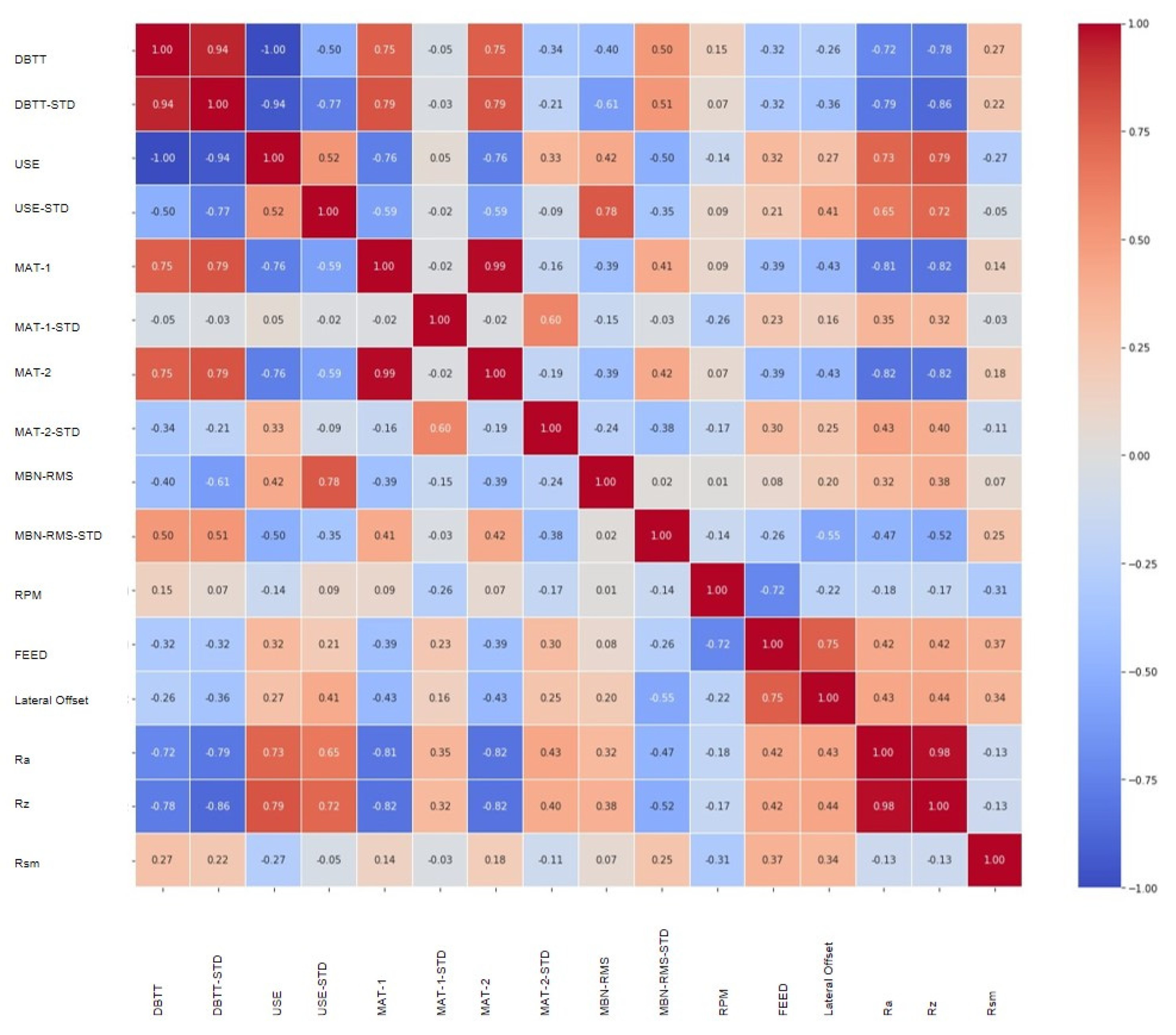
1.2.1. Exploratory Data Analysis

The first step is to look at the provided data and perform an Exploratory Data Analysis (EDA). This means examining the data to detect any missing values, to determine a relationship between the variables, and to take account of the data statistics such as mean, median, mode, and standard deviation [12]. There are two ways to perform EDA, graphically and non-graphically.

Since the dataset is new, the user may not have any idea about the underlying relations or even the patterns in the data. As the exploration is performed, some ideas may lead to interesting insights and some ideas may just be a ‘dead end’. There are generally two types of questions about the data, the type of variation that exists and the type of correlation that exists [13].

Graphical data analysis is best done in the form of bar charts for categorical data and histograms for numerical data [14], which is often easier to visualise than having a large array of numbers. Non-graphical data analysis is done by looking at the data statistics that include the central tendency—such as the mean, median, and mode, the spread of the data by looking at the standard deviation, and the shape of the distribution [15]. EDA also allows for the examination of the presence of outliers, which also shows the quality of the data.

Univariate analysis involves the analysis of a single feature. This analysis includes histograms, count-plots, boxplots, and violin-plots, and are known as summary plots since they show the frequency distribution of the data. 2D scatterplots and line-plots can also be used for univariate analysis by plotting the feature on the y-axis and their corresponding index numbers on the x-axis [16]. One very useful feature is the option of colour coding the data by groups in order to see the spread of each category.

Bivariate analysis involves the analysis of two variables (X, Y) and is the best way to determine the relationship between two variables. 2D scatterplots and line-plots can be used by assigning both the X and Y axis as variables and the data points can be grouped by labels. Pair-plots can be very useful to observe the correlation between more than two features. The study in [17] displays a pair-plot for visualising the Iris-Dataset, where a number of 2D plots are provided in a matrix format displaying comparisons of different data variable comparisons, albeit sequentially, and each plot’s comparing two variables to show the fitness of correlation between the two. Along the diagonal plots are histograms of the feature in their corresponding rows. This is a very powerful technique for visually displaying data correlations.

Variables can have a positive or a negative correlation. In a positive correlation, both the variables move in the same direction. An increase in X will also show an increase in Y. For a negative correlation, an increase in X results in a decrease in Y and vice versa. The closer the points are to the line of fit, the stronger to the correlation. However, if the line of fit is completely vertical or horizontal or there is no line of best fit, then there is no correlation between the features [18].

A similar way of showing correlations is with an Attribute Correlation Heat-Map. Among other methods, such as Kendall Tau and Spearman Rank, this method uses a Pearson correlation coefficient by default to calculate the linear correlation between two variables [19]. The resultant values range from −1 to +1, with +1 showing the strongest positive correlation. These results are presented as a matrix that can be plotted as a heat-map to clearly visualise the strength of the correlations [20].

1.2.2. Regression Models

Several different methods of imputation were tried; however, the method of choice for predicting the missing values and creating more data are by using a regression analysis. This is a predictive modelling technique that determines the relationship between the dependent and independent variables for analysis or even making predictions [21]. The benefit of using regression techniques is that, not only does it determine the correlation between the variables, but it also determines the contribution of each variable on the relationship.

1.2.3. Decision Trees, Random Forest, and Extra Trees Regression

One of the regression and classification models being used is called Random Forest, which is based on a bootstrap aggregation of decision trees. Decision trees work much like humans in the sense that the algorithm asks questions about the existing data to see where to classify the data or until it reaches a prediction, which is based on data regression [22]. A decision tree is a flow chart like structure where the interior nodes represent the features, the branches are decision rules with questions that are answered in either True or False, and the stopping criteria is realised based on the impurity of a split—for example, Gini or Entropy. An example of such decision trees can be found in [23], which displays how the rules are found from the root node to the interior and leaf nodes.

Random Forest fits multiple decision trees—hence the name Random Forest—on subsamples of the data and averages the decision trees to avoid over-fitting and improve the accuracy. The process of taking the mean of all the outputs is known as aggregation [24]. The benefit in using multiple decision trees comes from the ‘random’ attribute of the Random Forest algorithm. Each node in the decision tree works on a random subset of features and, as a result, each decision tree is individual.

The Extra Trees Algorithm is related to decision trees and the Random Forest Algorithm. The Extra Trees Algorithm, unlike the Random Forest algorithm, which takes bootstrap samples of the data, fits the algorithm’s overall data. Another difference is that it chooses where to split the nodes at random, whereas Random Forest chooses the optimal split for each node [25]. Splitting the nodes at random adds a random attribute to the Extra Trees, but it does increase variance. To work around this, the number of trees is increased [26]. Classification and Regression Trees (CART) work in a similar manner and are used to provide a second classification technique when testing improvements in performance when data augmentation is applied.

Another technique used to test classification of augmentation is the Neural Network (NN). The NN used in this work is a multi-layered perceptron with a backpropagation learning rule that is very similar to the work carried out [27]. Due to the nature of the problem being non-linear, an input layer of 8 nodes is used to cover the 8 input values. Three hidden layers at 16, 32, and 32 nodes, respectively, were used to segregate the non-linear relationships, followed by a pure linear output layer of 6 nodes. This was to cater to all the different output states.

Both techniques of CART and NNs are supervised in nature and used to investigate the differences in learning with both increased dimensions and applied augmented data to address such problems when presented with increased data dimensions.

This paper is divided into the following sections, the experimental setup for investigating the surface quality effects to Barkhausen noise, the Barkhausen noise applied to different surface quality Charpy samples with the effects suppressed using non-magnetic variable thickness spacers, data imputation and augmentation for low datasets, the results section—followed by a discussion of results—and, finally, the conclusions.

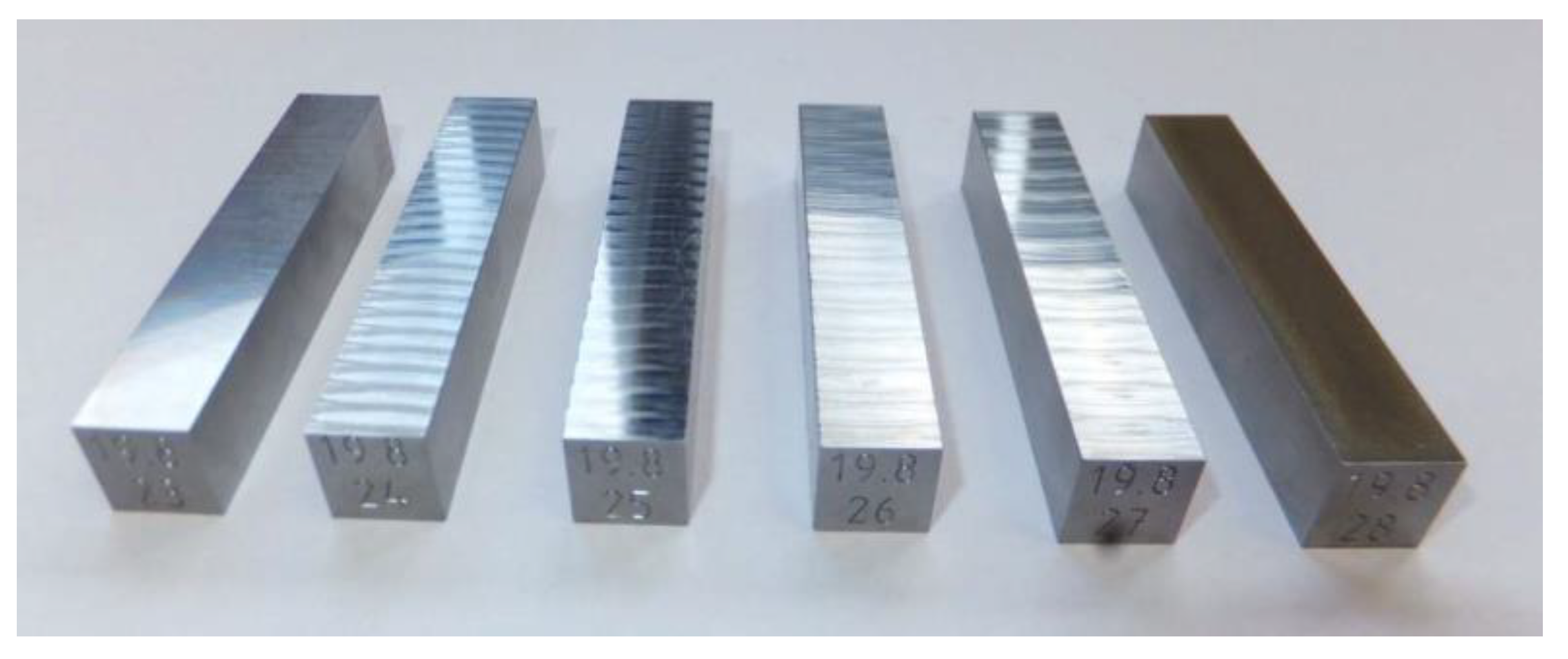
2. Surface Quality and Barkhausen Noise Sensor Experiment Setup

The fabrication of seven Charpy samples (displayed in Figure 1) without notches and with various manufacturing parameters (RPM, Feed rate, Lateral offset) was performed to deliberately modify the surface roughness and also “simulate” machining in a controlled area on irradiated samples that results in different surface conditions. The corresponding measured standard surface roughness parameters (R_a, R_z, R_sm) are shown below and are used as the calibration samples for the Non-Destructive Evaluation (see

Table 1. Material rotational speed and feed rates.

Sample No.		23	24	25	26	27	28
RPM	[t/min]	1000	500	600	500	600	EDM
Feed	[mm/min]	75	1200	1700	2000	2500
Lateral offset	[mm]	0.1	0.1	0.1	0.2	0.25
Average surface roughness (Ra)	[μm]	0.13	0.49	0.33	0.73	0.61	3.65
Maximum peak to valley height of the profile (Rz)	[μm]	0.83	2.33	1.59	3.9	3.3	19.56
Root mean square average of profile height deviations (Rms)	[μm]	77.6	129.1	244.3	382.2	195.3	127.3

).

Charpy samples of gradually increasing roughness were prepared from ferromagnetic steel in the shape of rectangular prisms (10 × 10 × 55 mm). Table 1 provides the information of how such samples were produced using a combination of different rotational and thrust forces (feed rates).

This not only gives different surface conditions, but it can also present different stresses within the surface due to different machined parameters (instead of effective cutting, a dragging effect can result) [8]. The machining of choice was face milling and the material for the samples was embrittled by thermal processing [28]. The quality of the surfaces for the samples corresponds to the machining process (milling) and grooves or even the scratches provided by that process with the objective of using different rotational and feed rates to obtain different surface roughness conditions. If one of those parameters, namely the rotational speed, are not fixed at a constant speed then a by-product of machining will exist, such as machine-induced residual stress. The final sample (sample 28) was produced from direct Electro-Discharge Machining, which resulted in the highest surface roughness value.

The ferrous yokes were attached to the surface of the samples either directly or over a thin spacer. It was found that the unwanted influence of the rough surface can be reduced by using a nonmagnetic spacer. The spacer can reduce or modify the feedback response, which inherently can influence the measurement. In fact, they substantially reduce the scatter of experimental points accompanied by a slight decrease of the overall degradation functions sensitivity. Spacers, in particular if they are thick, are able to modify the shape of the measured signals qualitatively and to bring about a considerable increase of sensitivity, especially in the degradation functions computed from the signal derivatives [8]. At the same time of mitigating against the surface quality, the received signal is reduced. This reduction is proportional to the change in the thickness of the applied spacer.

Experimental Setup

Dimensions samples 10 × 10 × 55 mm3      Material 22NiMoCr37      Orientation L-T      Engraving one side      Measuring device Accretech Handysurf Tokyo Seimistsu E-35B      Cut-off value 0.8 mm      Evaluation length 4 mm      Measuring range automatic

Barkhausen Noise

From the generated MBN measurements, other parameters are calculated and provide further discriminating quantities, which are used to further discriminate the material conditions. The MBN is an RMS magneto-elastic parameter (mp) that is expressed as a function of the magnetizing voltage, current, and frequency applied to the material under testing. A time window of several bursts would indicate a general response. The RMS of the MBN response signal is given by Equation (1):

$$RMS=\sqrt{{\frac{{\sum }_{i=1}^n{y}_i}{n}}^2}$$

(1)

where n is the total number of MBN signal bursts captured within a specified frequency range and y_i is the amplitude of the individual bursts.

Within the Rollscan 350 Analyser system [29] there are a number of parameters that need to be set for the stimulated electromagnetic waveform. Such parameters are voltage and frequency, as well as a high frequency pickup response filter. Taking advantage of the skin effect equation (see Equation (2) for more information), the lower the frequency, the greater the depth of penetration into the material. Both the magnetising voltage and frequency sweeps were undertaken to identify the optimum parameters based on the displayed material response. A penetration depth between 0.01 mm and 1 mm is achieved by using the frequency pickup filter of 70 kHz to 200 kHz. Using the Microscan software, repeated measurements were then recorded for 5 s of duration [30]. As displayed in other works, [31] describes the used Barkhausen parameters in greater detail. For replication, 2 V and 120 Hz were used as the exciting signal parameters for this surface quality study. This selection was based on previous tests investigating the detection of radiation-induced embrittlement, as well as being in good agreement with the frequency and voltage sweeps of the tested materials.

$$\delta =\frac{1}{\sqrt{\pi f\mu \sigma }}$$

(2)

where δ is the skin depth, f is the frequency in Hz, µ = permeability of sample, µ = µ₀ × µ_r, µ₀ is the permeability of free space at 4π × 10⁻⁷ H/m, µ_r = relative permeability, and σ is the conductivity in S/m.

The system being investigated is a commercial off-the-shelf-based system provided by [29] as being certified for repeatable use. The tests undertaken are similar to the tests carried out in [28], where the same sample set is being used to perform robust comparative studies. The output goal of this work was to be able to differentiate different surface qualities based on the detected electromagnetic response waveform. To address the uncertainty of measurements and, specifically, the conditions encountered in service, it was observed that the surface quality of the material has a considerable influence on the extracted sensor response. Therefore, to mitigate against these effects, a design of experiments should demonstrate the differences in sensor responses based on the material surface quality (the same base material will remain constant throughout the tests).

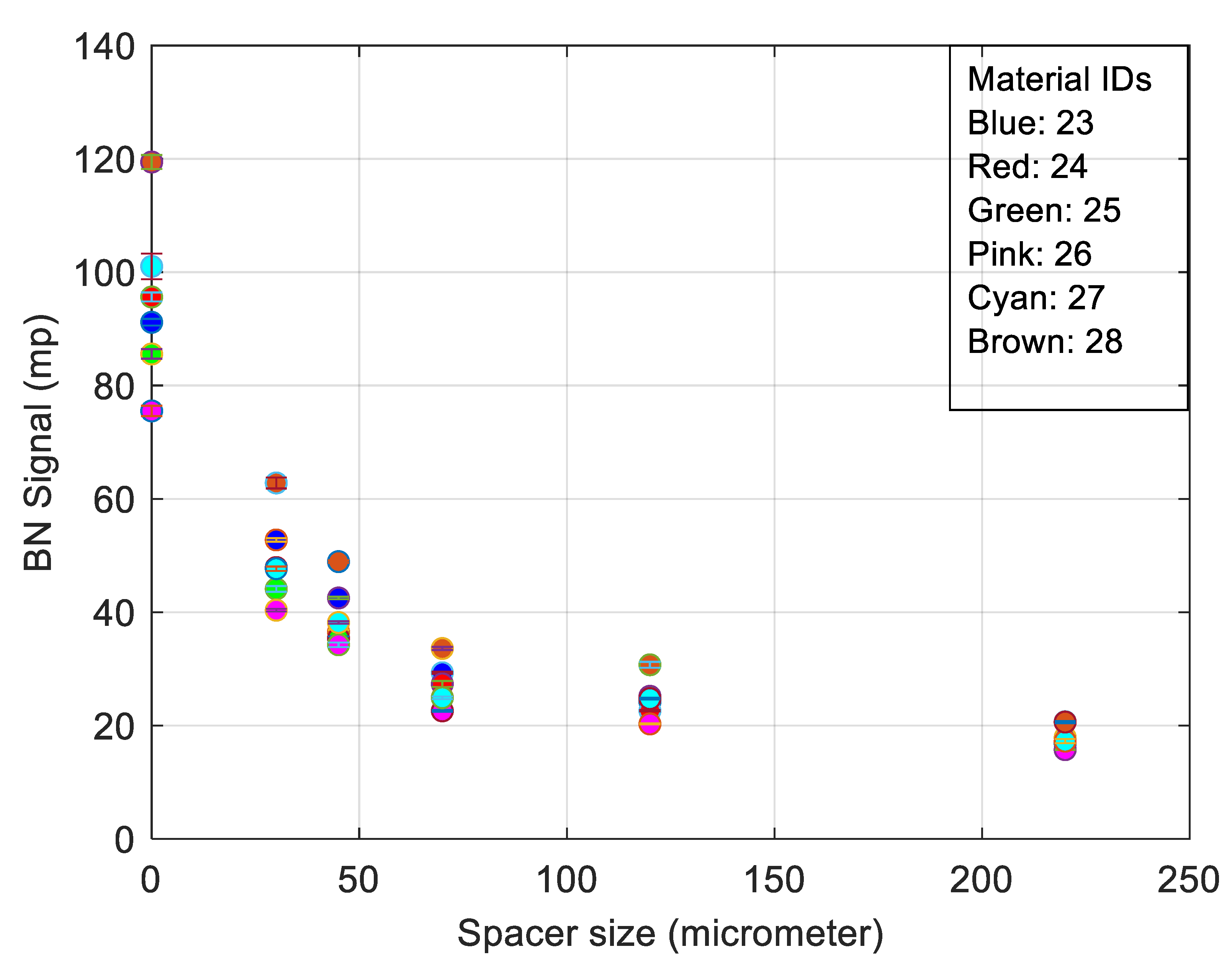
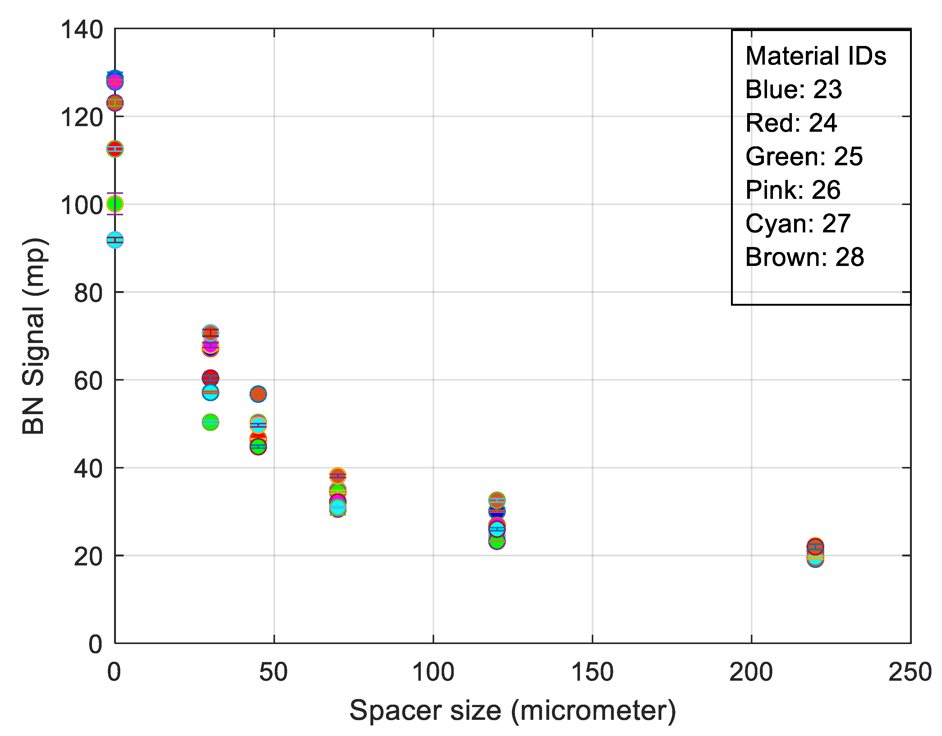
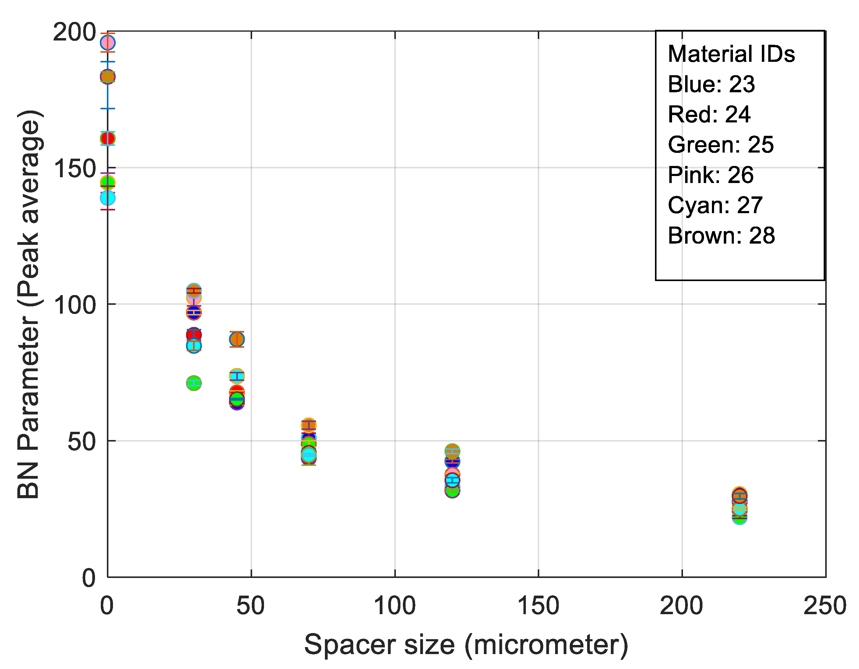
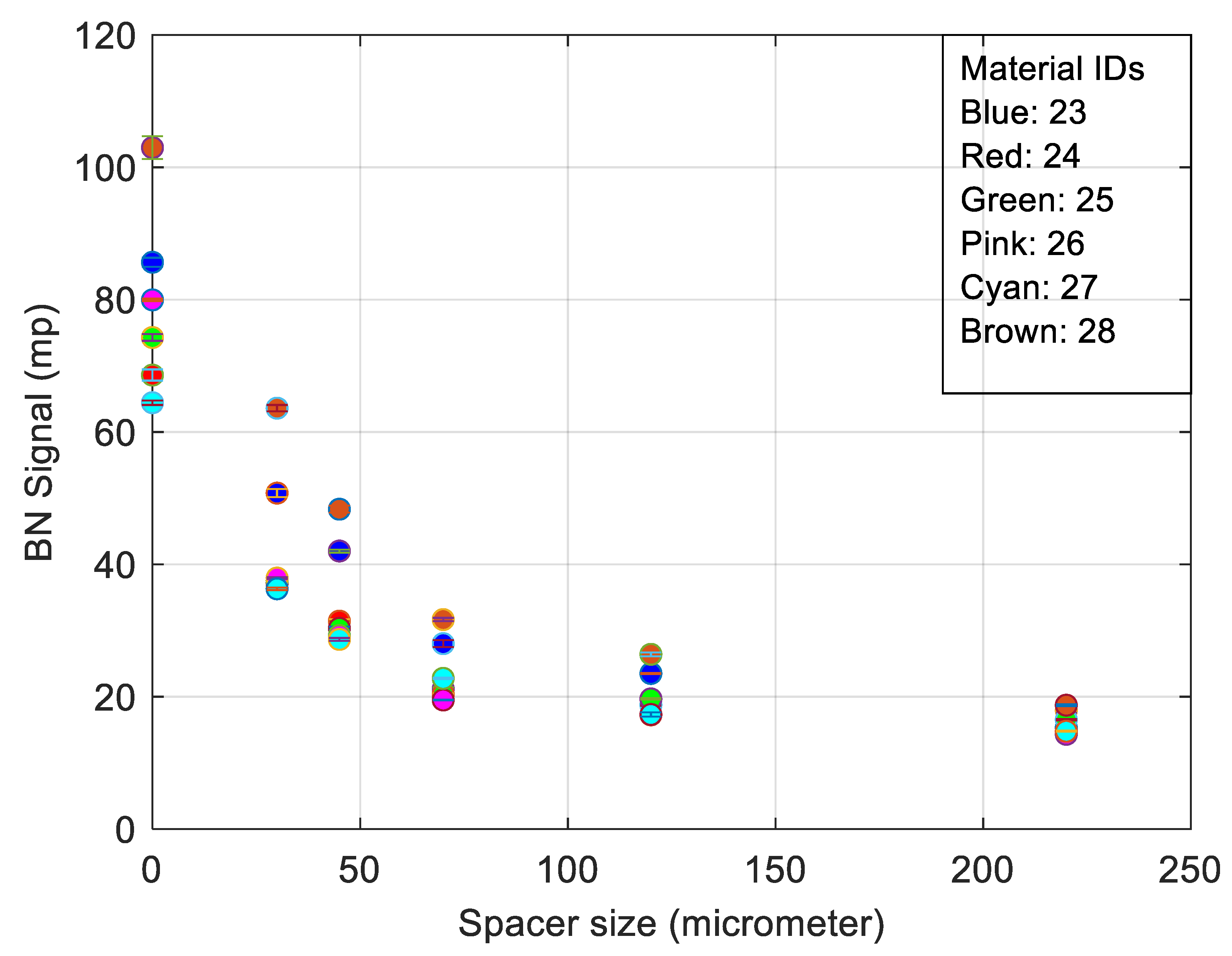
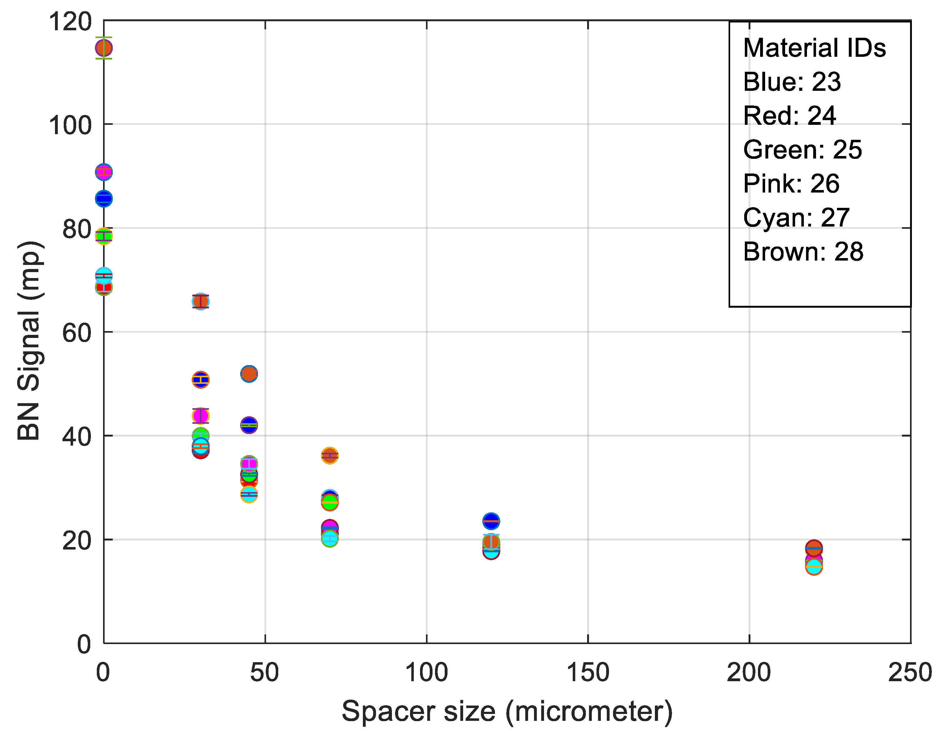
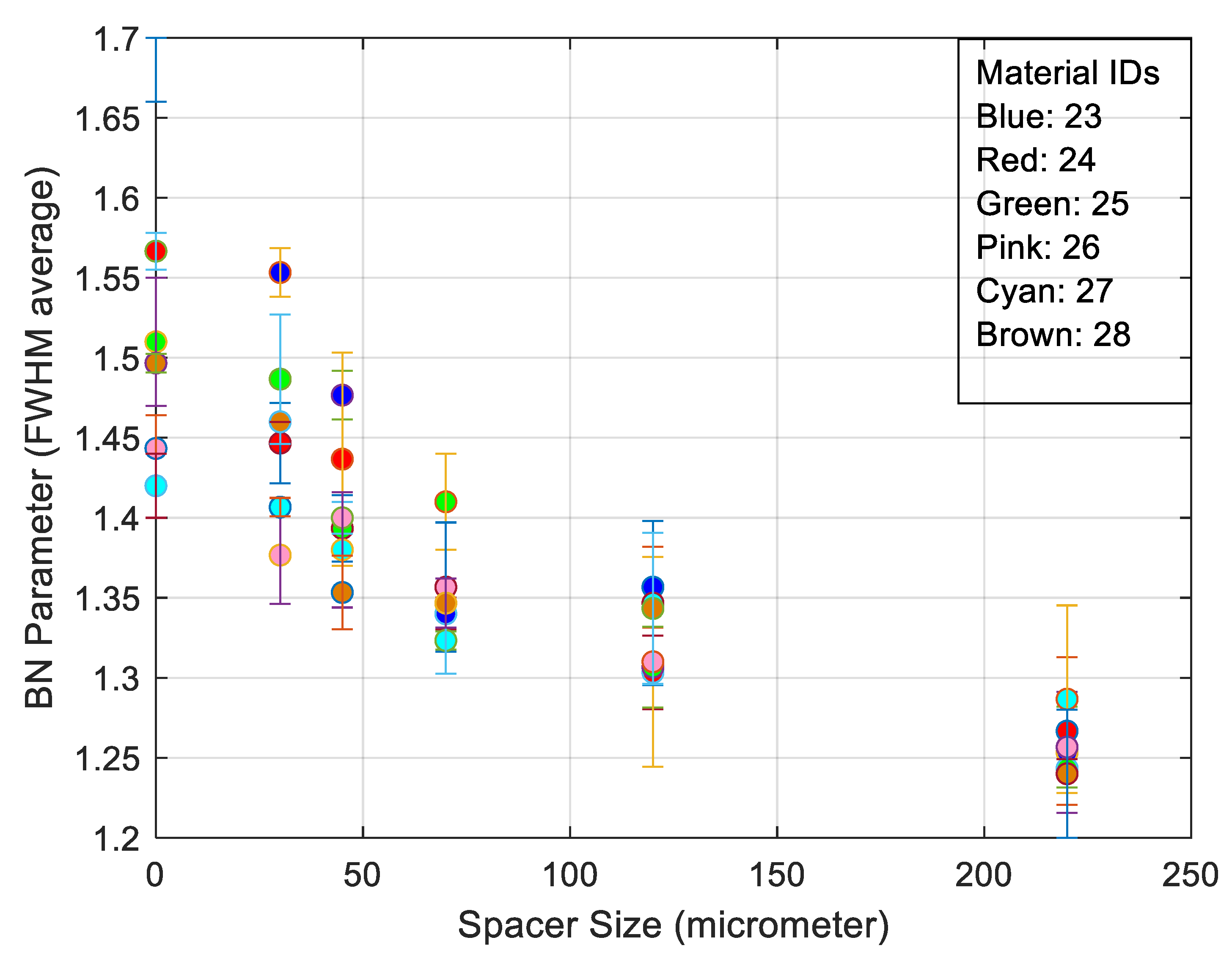
3. RMS Barkhausen Noise and Extended Measured Parameters Applied to Different Spacer Thickness

A series of BN measurements were carried out (1) without a spacer, i.e with direct contact of the magnetizing yoke and sample surface, (2) by applying a 30 μm thick nonmagnetic spacer, (3) by applying a 40 μm thick nonmagnetic spacer, (4) by applying a 70 μm thick nonmagnetic spacer, (5) by applying a 120 μm thick nonmagnetic spacer, and (6) by applying a 220 μm thick nonmagnetic spacer between the magnetizing yoke and sample surface.

The aim of the work is to investigate whether a correlation can be found between surface roughness and magnetic behaviour, and further evaluate the role of a spacer to reduce the effect of surface roughness by providing a uniform airgap. The evaluation was made through direct experimental results and machine learning paradigms.

The following Figure 2, Figure 3, Figure 4 and Figure 5 look at the varying RMS BN responses for the different materials with increasing surface roughness starting from material 23 to material 28 (see Table 1 and Figure 1 for more information). The four figures display top longitudinal and transversal measurements and the bottom longitudinal and transversal measurements, respectively, with both with or without spacers applied to the measurements.

Looking between the different machined parameters (different material IDs) without the use of a spacer (space size: 0), there is no clear distinction in terms of the surface roughness and BN response—except there is a lot of variation present from the returned RMS BN responses. The assumption here is the variation obtained is based on the surface roughness as the material has the same properties for each sample.

Figure 2, Figure 3, Figure 4 and Figure 5 show the test comparing no spacer (spacer size = 0 on the plots) and then a 30 µm thick spacer with varying increments of up to 220 µm. These figures display the effects of using different thicknesses of spacers to suppress the influence of the surface roughness and reduce the variation to improve the overall results. At the point of 220 µm, this could be considered as the limit for the BN electromagnetic process where the retrieved response is tending towards the levels of background electromagnetic noise (where any BN reading that is within 5 times of the background noise is ignored).

The useful role of nonmagnetic spacers for suppressing the effects of varying surface qualities was demonstrated by viewing Figure 2, Figure 3, Figure 4 and Figure 5. With different levels of surface roughness allowed, a study can be conducted in terms of what are the influencing effects when carrying out Barkhausen noise measurements and the associated decrease in surface quality. This is particularly important when considering the actual in-service conditions, given such differences in the surface quality or oxidation effects from a harsh environment. A number of constants were adopted to understand these phenomena of interest, and, in this case, the surface quality was considered to be most important. The material, the machining process, and the Barkhausen parameters (frequency and voltage magnitude) all remained the same throughout.

The experimental work displayed a good correlation between different surface roughness conditions. Figure 6, Figure 7 and Figure 8 display the extended parameters of BN and were used to increase the data dimensionality to display such effects. These figures display their correlation with the RMS Barkhausen noise signal, as well as provide data to test the effects of the increased data dimensionality applied to the machine learning techniques. Figure 8 appeared to give the best correlation of surface roughness where the measured signal response correlated with the measured surface roughness and sample 23 was considered an outlier throughout with other effects influencing the BN response (this was the only sample to receive a much higher RPM in manufacturing the surface quality). With sample 23 eliminated, there are clear distinctions from sample 24 (second lowest BN and Ra) to sample 28 (highest BN and Ra). As an initial study, the experimental results can be concluded as a success.

The next section applies machine learning techniques, such as Neural Networks (NNs) and Classification and Regression Trees (CART), to further reinforce these results.

In order to test both ML techniques, there is a need to increase the data dimensionality where the extended parameters are as follows:

• Full width half maximum (FWHM) provides a full width at half the max of the filtered burst signal.
• The peak average is the peak of the filtered burst signal over the defined number of bursts, thereby giving a windowed average value.
• The spectrum is calculated from the raw Barkhausen data. The block size is selected so that it is to the power of two and less than the length of the data. The maximum size is currently set as 2¹⁵. The spectrum calculation is applied for each block so that the blocks overlap by half. First, the Hamming window is seen in Equation (3).

$$y_i=\left[0.5-0.5\cos \left(\frac{2\pi i}{n-1}\right)\right]\left[0.5-0.5\cos \left(\frac{2\pi i}{n-1}\right)\right]y_i$$

(3)

is applied and then the spectrum is calculated as seen in Equation (4):

$$ps=\frac{{\left|FFT\left(X\right)\right|}^2}{n^2}$$

(4)

where ps is the power spectrum and FFT is Fast Fourier Transform.

The sum of spectrums over the blocks is averaged and then scaled, as seen in Equation (5):

$$p{s}_i=4\sqrt{p{s}_i}$$

(5)

Then, the spectrum area is the integral of the spectrum data.

Figure 4 was identified as the best BN response in terms of the placed sensor direction to distinguish the different surface material conditions, and, for these reasons, the extra parameter study was carried out for this measurement (bottom surface, transversal sensor orientation). Figure 4 is based around the transversal measurements from the bottom side, and hence why Figure 6, Figure 7 and Figure 8 are extra parameters obtained for the bottom surface and transversal measurements and should give more distinguishing features that are all correlated with the RMS BN response of Figure 4. These results provide an information structure for discerning which signal responses relate to which material and associated surface quality. The information correlated is in terms of the extra dimensions of the data. This data is therefore considered useful for studying the effects of n-dimensionality on data, and from increasing the data with augmentation to overcome such effects. Section 5 will explore these effects in terms of the two chosen machine learning techniques of NNs and CART. First, Section 4 looks at data augmentation in the form of the imputation of missing data provided from similar electromagnetic quantities, such as those given by the MAT technique.

4. Machine Learning Applied to Imputation and Data Augmentation to Increase Classification Accuracy

4.1. Methodology

The values for the surface roughness metrics were provided for samples 23 to 28. These values are added to a constraint database after grouping the materials by MATERIAL_ID. By adding these values to the database, it enables the observation of the effects of surface roughness on all the magnetic measurements within the dataset. This approach also makes use of other input variables for the samples that were not tested in order to increase the sample size.

The data is then predicted in two segments. The first segment containing values for R_a, R_z, and R_Sm, and the second segment containing the machining parameters. The surface roughness parameters are predicted first since they have fewer Not a Number representations (NaNs) compared to the machining parameters. NaNs are provided when numerical data cannot be provided.

An EDA is performed before and after predicting the NaNs in order to observe the correlations and how and if they have been changed after populating the data.

4.2. Preliminary EDA

The heat-map of Figure 9 displays the correlations between the variable before the NaNs are predicted. The reason there are blanks in the plot is because there isn’t enough variation in the DBTT and USE columns to determine a correlation. The heat-map shows a strong positive correlation between Ra and Rz with Ductile to Brittle Transition Temperature (DBTT), Upper Shelf Energy (USE), and its standard deviations and negative correlations with MAT_1, MAT_2, and the output values of the MAT method. Lateral Offset and Feed shows strong negative correlations with MAT_1 and the correlation weakens with MAT_2. (MAT_2 is the raw output value of MAT method, i.e., the value of the selected magnetic descriptor. MAT_1 represents a degree of variation so it is normalized to a value that was obtained from the reference sample).

The initial pair-plot displaying the distribution plots are all skewed positively or negatively. There is a clear positive linear correlation between MAT_1 and MAT_2. MAT_2 and MBN_RMS have a correlation with R_a and R_z. Not only does the EDA display a strong data correlation between both MAT and MBN, but both are also very much different methods in principle, where the former provides current/permeability loops of the bulk sample measurement and MBN and the Barkhausen response of the point space of the sample measurement. This correlation of the two methods provides a strong value, especially when imputing data. There does also seem to be a correlation between MBN_RMS and Feed, but there is not enough data to visualise a correlation on a scatterplot.

Prediction Results

The heat-map of Figure 10 shows a correlation between the variables after prediction. R_a and R_z show strong negative correlations with DBTT, MAT_1, and MAT_2 after predictions. R_a and R_z also show positive correlations with USE. The correlations between RPM, Feed, and Lateral Offset and MAT_1 and MAT_2 have been reduced by the variance of the predicted data. In cases like RPM and MBN_RMS, the correlation has changed from negative to positive.

Pair-plots display very similar information to that displayed by Figure 9 and Figure 10 where correlations are apparent from pattern linearity. If, however, the visualised paired data displays just data points with no linear patterns, then there is no correlation between those specific data pair parameters. Pair-plots have not been shown as the data are very similar to Figure 9 and Figure 10 (same parameter variables for the x and y axis and, instead of a number relating to a correlation metric, all the data points are displayed) and, with many subplots nested in an overall plot, it is difficult to see the subplot information. As an observation of the pair-plot results, the spread of the data have decreased as the data are concentrated to add skew to the plots. In the scatterplots there are new groups of data, such as the USE and RPM plot where there are additional vertical lines.

The full pair-plot displays the distribution plots, which are all skewed positively or negatively. There is a clear positive linear correlation between MAT_1 and MAT_2, which is more prominent than the initial preliminary pair plot. MAT_2 and MBN_RMS have a correlation with R_a and R_z. Finally, there does seem to be a correlation between MBN_RMS and the Feed rate.

From using such techniques, it is possible to ‘fill in’ missing values and increase datasets in an intelligent fashion. With the correlations provided by either metrics or data pair correlation patterns, it is possible to gain more confidence in terms of imputation of missing data.

4.3. Machine Learning Applied to Surface Roughness Prediction

The machine learning techniques of Neural Networks [32] and CART [27] were used to classify different levels of surface roughness based on multiple Barkhausen noise parameters for different spacer sizes. Trice measurements conforming to the minimum repeatability were carried out. Surface roughness has been used as a parameter output, however, the material sample number associated to a known measured defect could have been used also. Not only the classification of the surface roughness has been chosen as a test, but also increasing the dimensionality to see the effects of diminished accuracy and to combat against this, there is use of data augmentation for reinforcing learning paradigms that build on the already empirically obtained sensor data.

4.3.1. Neural Networks, n-Dimensionality and Augmentation

The following results tabulated in

Table 2. Neural Network results for normal data and different levels of dimensionality and augmentation.

Data	Data Size (Columns)	SSE	Distance Error	Time to Train	Unseen Test Case Accuracy	Iterations	% Aug * Increase
mp (Tx)	98 (2)	7.31 × 1016	−0.02633	0:04:48	20/20	20,000	0
mp (TXLx)	98 (3)	6.65 × 1015	−0.02454	0:04:46	19/20	20,000	0
mp (TxLx) & Param	98 (6)	4.24 × 1014	−0.77117	0:05:11	17/20	20,000	0
mp (TxLx) & Param & Augmented	108 (6)	6.09 × 1011	−0.33589	0:10:26	18/20	20,000	10
mp (TxLx) & Param & Augmented	118 (6)	1.00 × 1010	−0.28471	0:10:30	17/20	20,000	20
mp (TxLx) & Param & Augmented	158 (6)	1.10 × 109	−2.54116	0:12:10	13/20	20,000	60
mp (TxLx) & Param & Augmented	205 (6)	6.03 × 109	−5.31443	0:12:46	11/20	20,000	100
mp (TxLx) & Param & Augmented	158 (6)	2.80 × 1012	−2.32811	0:11:39	17/20	20,000	60 **

Key: * Aug = Augmentation; ** Other half of data; Tx: Transversal measurement; Lx: Longitudinal measurement.

display a standard feedforward, backpropagation NN that was tested with a base level amount of data and, from that base level, through increasing the n-dimensions and then increasing the data with applied data augmentation. From increasing these different levels of data, both the accuracy and sum-squared errors (SSE) were used to display progress. The sum-squared error can be a little misleading, therefore the distance measure where the sum of the difference between the predicted value and the real value gave the distance error value (all summations relate to the negative distance); this is more of an indication of accuracy and learning capability. In addition, a scaling max-min algorithm was used to provide normalised scale data to ensure that no one dimension was more biased than another and a fair comparison of tests was carried out.

The Neural Networks used were four layer networks with two hidden layers. The input layer was 6 neurons (number of neurons to mimic the input data), with the hidden layers increasing to 36, 72, and 36 neurons respectively. The output number was based on the number of output values/classes. These values were chosen to address all the different pattern variations between the presented input data. All of the neuron transfer functions for the first three layers used tan-sigmoid and for the final output layer pure-linear was used. In terms of the neural network parameters, maximum epochs were set to 20,000, learning rate set to 0.1 × 10⁻¹⁰, momentum set to 0.8, and finally, in terms of learning rules, the resilient backpropagation along with the Kohonen weight learning function was used for training the network. The input layers had been chosen to be more than the amount of input variables due to the nature of the data, where there are different measurements made from using different layer technologies, which are included and this needs to be considered when segregating the total pattern space. Also, by using a trial-and-error approach, six neuron inputs for the associated hidden layers did not provide useful results, whereas thirty-six neuron inputs gave a good account and trade-off against further increases. Using this trial-and-error approach to display the performances, metrics were obtained from testing the network with unseen data. Such results are used to display data generalisation as opposed to data fitting.

As can be seen with Table 2, as the n-dimensionality increases, the level of accuracy and SSE starts to decrease, so one can even conclude with correlated data inputs the increase in dimensionality has an effect on accuracy and trend-based learning. To overcome this, the use of data augmentation was used where data amounts were increased to give more general capabilities to the machine learning techniques. Despite n-dimensionality affecting the error distance measure, data augmentation starts to decrease the error distance measure, albeit the SSE remains similar. This suggests data augmentation is a very useful tool for providing more trend learning capabilities. That said, if too much of an increase is used, this can also be detrimental to the learning process. With a 100% increase in augmentation, the error distance measure is at its worst along with SSE, however, if the data amounts are modest—such as a 10% or 20% increase—then improvements in the error distance measure can be obtained. The SSE is less for larger amounts of data, and this is due to the same network having more cases to consider and overfitting instead of learning. One important aspect to note was the simplistic augmentation algorithm used to produce such values, which was based on the mean and the standard deviation of the measurements. Such a basic algorithm was chosen for this initial study to provide full transparency and understand the effects of data variation. A test of 60% augmentation was made for the first half of the data, and then the second half of the data. Interestingly, the second half of the 60% augmentation performed much better than the first half of the 60% augmentation. The difference being the second half of data augmentation at 60% had more data that varies more dramatically than the first half of data augmentation at 60%, and therefore provided a better learning coverage.

4.3.2. CART, n-Dimensionality and Augmentation

CART was used as a second machine learning technique to get a different perspective of learning capabilities when compared with neural networks.

Table 3. CART results for normal data and different levels of dimensionality and augmentation.

Data	Data Size (Columns)	Distance Error	Unseen Test Cases	% Increase of Augmentation
mp (Tx)	98 (2)	0	20/20	0
mp (TxLx)	98 (3)	0	20/20	0
mp (TxLx) & Param	98 (6)	0	20/20	0
mp (TxLx) & Param & Augmented	108 (6)	0	20/20	10
mp (TxLx) & Param & Augmented	118 (6)	0	20/20	20
mp (TxLx) & Param & Augmented	158 (6)	−2	17/20	60
mp (TxLx) & Param & Augmented	205 (6)	−2	17/20	100
mp (TxLx) & Param & Augmented **	158 (6)	−1.2	18/20	60 (other half)

Key: ** Other half of data; Tx: Transversal measurement; Lx: Longitudinal measurement.

gives similar output measures to Table 2 to be able to give a good comparison. That said, classification trees were more suited for this type of data than NNs, as the ‘curse of data dimensionality’ has less of an affect when compared with NNs. The distance error measure, however, increased as augmentation percent levels increased—also, the unseen test case accuracy started to decrease. As the results are somewhat similar to NNs, this second machine learning technique further reinforces the findings of the increases in dimensionality and augmentation in terms of accuracy and learning capability.

The classification tree for the Transversal or Longitudinal sensor orientation BN (mp) values promote much smaller trees due to the amount of information present. With extra parameters provided by the focused Transversal BN values, the classification tree increases and caters for more complex demarcation when differentiating more data with a higher confidence of the phenomena under measurement. With augmentation of the data, the rules and complexity increase, however the demarcation of boundaries within the measurement are also increased. The augmentation forces X1 and X2 variables to segregate the different surface quality outputs, where only X1 is used for sole transversal measurement data information. Having extra parameters provides more data dimensions for segregating the information of interest.

A divide-and-conquer approach was not necessary to classify any overlapping data groups as the unforeseen combined data were also predicted with a 100% accuracy. From these results, it can be concluded that surface roughness can be correlated to different material samples, which could be used to add or subtract such effects from an overall NDT model or assist in furthering the understanding of magnetic effects with magnetic sensing technologies.

All of the ML metrics were considered to be connected where they all gave a similar pattern to the learning capability. For instance, from Table 2 it can be seen that for a single dimension of data the sum-squared error (SSE), see Equation (6), distance error, see Equations (7) and (8), and the accuracy of the unseen test data all give the most favourable results where SSE is the lowest, distance error is the lowest, and the unseen test data are at the highest. Finally, the R² statistical metric is used to provide a best fit for the unseen test set of each test.

$$SSE={\displaystyle \sum }_{i=1}^n{(X_i-\overline{X})}^2{}_{}$$

(6)

where X_i is the actual measured response state, $\overline{X}$ is the mean measured response, and n the sample size.

The distance error was calculated from Equation (7), and the total distance error was calculated from the following Equation (8):

$$D_i=(T_{Di}-T_{Ai})$$

(7)

$$D_T=\frac{1}{14}{\displaystyle \sum }_{i=1}^{14}{(D_i-{\widehat{D}}_i^{\left(-i\right)})}^2{}_{}$$

(8)

where T_A = Actual Target, T_D = Desired Target, D_T = Total Distance Error, and D_i = Distance Error for Target i.

$$R^2=1-\left(\frac{{\displaystyle {\displaystyle \sum }_i}{\left(a_i-p_i\right)}^2}{{\displaystyle {\displaystyle \sum }_i}{p}_i^2}\right)$$

(9)

where a_i is the actual measured wear state, p_i the predicted wear state, and n the sample size.

5. Discussion of Results

This section discusses three sections, where the first looks at obtaining data from a surface roughness suppression experimentation where different thickness spacer technologies are used to trade off between surface roughness issues and sufficient levels of the signal-to-noise ratio. Secondly, there is work presented on data imputation where graphical techniques display data dimensional correlations between different NDT measurement techniques and provide confidence when imputing NaNs. Finally, the last section looks at data augmentation applied to machine learning techniques to improve accuracy against ‘the curse of dimensionality’.

5.1. Barkhausen Noise and Extended Parameters Applied with Surface Roughness Suppression Techniques

The work presented here looks at the effects of using different thicknesses of spacers and how surface roughness can be mitigated to distinguish different material phenomena. In addition, such technologies could play a role in better understanding the effects of electromagnetic measurements, as well as providing predictions to remove or add unwanted material characteristic effects.

By using ML, it was possible to identify the surface roughness based on the magnetic feedback signature when noting the different spacer thickness. Such a method could be used to apply intelligent filters or be used to assist measurements where the trade off in the signal-to-noise ratio is negligible when the thickness of a spacer is very thin. With thicker spacers, it was more difficult to apply the machine learning techniques as the data was less discernible. Such types of work are very important to address the uncertainty of measurements, especially when faced with different levels of surface quality. Most NDT methods suffer from various levels of uncertainty—by identifying some of these and minimising the effects, the measurements become more consistent and repeatable. This is very important when applying such technologies to the safety of critical structures such as those seen in NPPs.

5.2. Graphical Techniques for Data Imputation Verification

It is often the case with NDT multiple sensor data applied areas that are difficult to access, such as RPVs in NPPs, where the obtained data is very small in nature and the dimensions (from the various applied techniques) can be very large. Here, imputation of missing data have been used to address such gaps in an intelligent manner. Section 4.2 displays some visual techniques, such as correlation heat-maps to show the individual data correlations of different sensor data before imputing values. The imputation was only considered for the Barkhausen noise (mp) mean value and no extra parameter or other NDTs. The extra sensor data obtained from NDTs along with other Barkhausen noise data provided intelligent imputation. Decision trees were considered to be the best technique for providing imputation values and were used to provide the results displayed in Section 4.2.

Finally, it was noticed that there is very little information on the imputation of sensor data in the literature, whereas this is becoming more and more of an important area when applied to NDT and continuous monitoring systems. There is, however, plenty of work on imputation when applied to image analysis, especially for automated vision for automobiles.

Both heat correlation and full pair-plots displayed strong data correlations, especially when such techniques were applied to the imputed data compared with non-imputed data. Such visual correlations give confidence to the applied techniques and, in short, validate the replaced NaNs.

5.3. Data Augmentation Applied to Machine Learning Techniques to Increase Accuracy When Faced with the ‘Curse of Dimensionality’

By using two different machine learning techniques, it was possible to see the effects of data n-dimensionality increase as well as the effects with different levels of data augmentation to impede the increase of data dimensionality. It was also found that the type of produced data augmentation plays a role in learning, where larger varying cases are better than smaller varying cases.

CART, however, did not suffer from the ‘curse of n-dimensionality’ given that the segregation rules were able to provide a more accurate representation and, therefore, a conclusion can be made that classification trees appear to handle n-dimensionality better than NNs. As already mentioned, this is further reinforced as the data given to both classifiers was pre-processed using a scaling max-min algorithm to provide normalised scaled data, as opposed to just standard raw data. In addition, the nature of this specific data are all correlated from the first dimension in that they all rely on the same specific measurement and are not from other sensors or different measurements (Barkhausen RMS noise and extended parameters). The NN, however, displayed diminishing learning capabilities from an increase in n-dimensionality. However, using small levels of augmentation with greater extreme variations gave the best results (see Section 4.3 for more details).

As the dimensions of data increase by considering not only the BN mean average response but also the selected extended BN parameters, the SSE starts to increase as does the distance error and the unseen test data cases, which decrease. These entries within the tabulated data display the changes in accuracy and ‘the curse of dimensionality’. From using a basic method of data augmentation to increase data and reinforce key data patterns, metrics can be used to see the accuracy given by these methods. With a 10% increase in data augmentation, the most optimised SSE, distance errors, and unseen test case accuracies were found. By increasing the data augmentation further, the data metrics were less in favour. This was thought to be due to data fitting through too much data augmentation, and more work is required here to see why this is the case. This investigation will be considered in future work.

By investigating these differences further, two studies were carried out with 60% augmentation, where one of the augmented datasets had very small differences in the change from the original dataset, and the other 60% with larger differences (more extreme with in the standard deviation (SD) limits). The one with more extreme data augmentation gained better SSE and a 20% increase in accuracy for unseen data cases. The distance error, however, was less favourable where it was slightly higher. The distance error metric suggests that the extreme augmented values may score better with an increased network size and iterations to learn the more complex, extreme data patterns. For this study, the network and iterations were all kept constant to make fair comparisons.

Another ML technique was used to test the same augmented data as used with the NN—the metrics can be seen in Table 3. The metrics in the case of CART were a lot more favourable with this technique. Similar to NNs, CART is also a supervised technique, however, it provides rules for segregation, which, in a lot of cases, are more robust than producing a boundary curve to segregate data. SSE, however, is not measured here as no iterative input to output mappings occurred with this method in comparison. In short, cumulative SSE is predominately used for large iterative learning techniques such as NNs.

It can be seen that a slight increase in data augmentation gives similar results to the NN, where 10% and 20% give 100% accuracy with both the distance error and unseen test cases. Beyond 20% data augmentation, the distance error and accuracy on unseen data all increase and decrease, respectively. Here, there are no real differences for both 60% augmented datasets. However, there is a slight increase in the distance error and a decrease in the accuracy for extreme augmented data, which could be due to the increase in complexity of the data patterns as seen with NNs.

Table 4. Comparison metric results for NN and CART techniques using different levels of data augmentation.

Data	Data Size (Columns)	% Aug * Increase	(NN) Sum Squared Error (SSE)	(NN) R2	(CART) R2
mp (Tx)	98 (2)	0	7.31 × 1016	1	1
mp (TXLx)	98 (3)	0	6.65 × 1015	0.9998	1
mp (TxLx) & Param	98 (6)	0	4.24 × 1014	0.8338	1
mp (TxLx) & Param & Augmented	108 (6)	10	6.09 × 1011	0.9939	1
mp (TxLx) & Param & Augmented	118 (6)	20	1.00 × 1010	0.9929	1
mp (TxLx) & Param & Augmented	158 (6)	60	1.10 × 109	−0.0168	0.0882
mp (TxLx) & Param & Augmented	205 (6)	100	6.03 × 109	0.3156	−1.23
mp (TxLx) & Param & Augmented	158 (6)	60 **	2.80 × 1012	0.3220	0.509

Key: * Aug: Augmentation; ** Other half of data; Tx: Transversal measurement; Lx: Longitudinal measurement.

displays R² metrics, which provide the results with another view in terms of accuracy from the prediction side of the test data and the best found fit. MAE was also found; however this gives a similar linked metric to R² and, therefore, a duplicity of results. Looking at Table 4 backs up the results discussed in this section, where 10% and 20% data augmentation give a better fit than without augmentation. However, increasing that data to much greater levels, such as 60% and 100%, creates more noise and diminishes the accuracy. Also, the results reinforce the extreme boundary data augmentation set compared to a normal boundary data augmentation set (for the two different 60% data augmentation sets). In the case of 100% augmentation, there is a higher score for NN and much less for CART, where a −1.23 is reported for R². The latter is significant to no real best fit and unable to give a sound prediction, whereas the NN is not that good, tending towards 0; however, there is some fit of the predicted data. This can be explained by the nature of the two techniques where the NN produces a boundary condition for the outputs and CART will have hard found rules that may not be able to fit the more complex data where overlaps or near overlaps exist.

There are two methods discussed in Section 4.3, where imputation and augmentation can be used. The results displayed in Section 4.2 and Section 4.3 display the transparency in producing such results as well as the trade-offs between extra data and extra n-dimensionality. This is very important as such data techniques cannot be applied in such a blind and ad hoc manner as there needs to be an evaluation, especially as this data are expected to be applied within a safety critical environment. If a good understanding and transparency is found within the produced data, then this should serve in reinforcing the machine learning techniques. The key idea behind data augmentation is to promote more accurate machine learning models through giving more extreme cases to allow rules to be more salient and with little to no ambiguity.

For safety critical components, it is important to characterise the presence of any surface defects including cracks, manufacturing flaws, service-induced cracking, or suspected degradation, as these defects can initiate and grow during service and may cause catastrophic failure by fracture. Hence, most of the structural integrity assessment methodologies tend to be highly conservative. By accurately predicting the surface quality levels, it is possible to obtain more reliable NDT measurements that can avoid being overly conservative with fracture assessments, and thus improve the possibility of life extension of existing power plants. Looking at both techniques and results given in Table 2, Table 3 and Table 4, the results are not 100%, however the predictions are within the required thresholds. The measurements of concern would be based on a range of historic measurements where damage would display a decrease and greater level of confidence. Nevertheless, whilst such NDE techniques mature, Destructive Testing would still be carried out until a level of confidence can be passed with that of NDE techniques.

6. Conclusions

In this work we demonstrate the effects of using spacers to reduce the effects of surface quality when carrying out electromagnetic measurements.

• The best trade-off between electromagnetic response and surface quality was found to be a 30 µm nonmagnetic spacer (Figure 6).
• It is often the case with such measurements that small sets of data exist in terms of describing the different anomaly conditions. For these reasons there was a need to find missing data usually in the form of ‘Not a Number’ or NaNs. By using advanced imputation algorithms, it was possible to impute missing values by intelligent interpolation and the use of other NDT data, such as that provided by Magnetic Adaptive Testing.
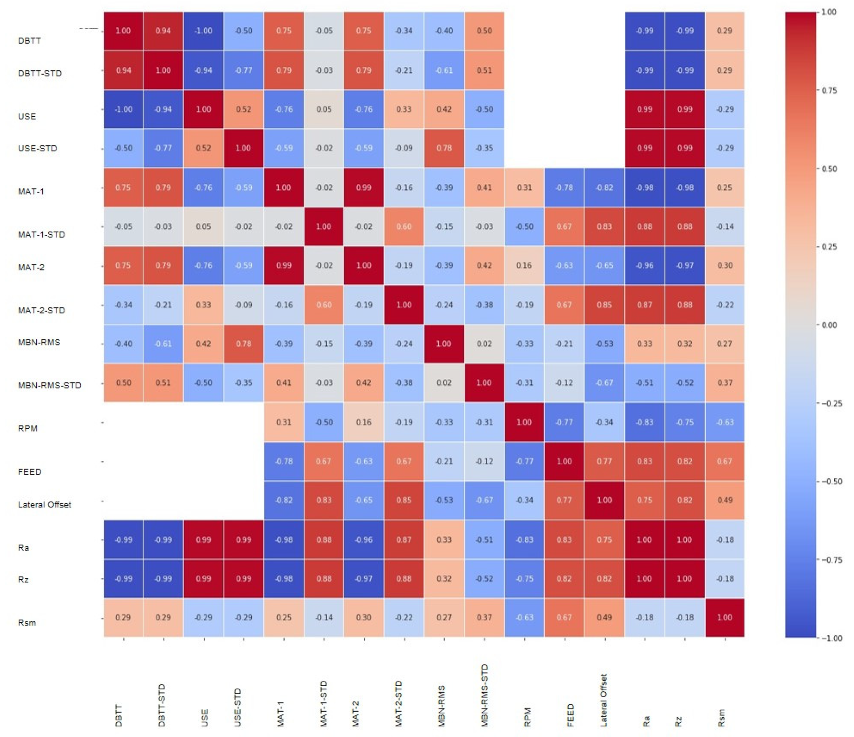
• In addition, by using statistical measures it was possible to apply the graphical correlations before making the predictions and imputing the missing data. Such techniques increased the data amounts and were considered to give good coverage and further useable data.
• Further to these findings, it was possible to see the effects on small datasets when n-dimensionality increases due to different parameters given within an NDT measurement, thereby providing more output values. Generally, the increase in dimensionality reduces the capacity for machine learning algorithms to provide generalistic pattern trend fitting capabilities. With the consideration of adding subtle data augmentation amounts (20% augmentation), it was possible to increase trend fitting capabilities. Beyond 20% augmentation, diminishing returns were obtained.
• Furthermore, studies of the data augmentation found that more extreme varying data amounts were better than slight varying data amounts.
• On a final note, classification and regression trees gave the best account when compared with neural networks in coping with the ‘curse of dimensionality’ when n-dimensional data increases.
• Future work will look further into more advanced algorithms to see how increased data can facilitate trend pattern learning as opposed to suppressing it. Also, further investigations into higher levels of data augmentation give reduced accuracy.

References

1. Kronmüller, H.; Fähnle, M. Micromagnetism and the Microstructure of Ferromagnetic Solids; Cambridge University Press: Cambridge, UK, 2003. [Google Scholar]
2. Jiles, D.C. Magnetic Methods in Nondestructive Testing: Encyclopedia of Materials Science and Technology; Elsevier Press: Oxford, UK, 2001. [Google Scholar]
3. Lo, C.C.H.; Jakubovics, J.P.; Scruby, C.B. Non-Destructive Evaluation of Spheroidized Steel Using Magnetoacoustic and Barkhausen Emission. IEEE Trans. Magn. 1997, 33, 4035–4037. [Google Scholar] [CrossRef]
4. Kikuchi, H.; Ara, K.; Kamada, Y.; Kobayashi, S. Effect of Microstructure Changes on Barkhausen Noise Properties and Hysteresis Loop in Cold Rolled Low Carbon Steel. IEEE Trans. Magn. 2009, 45, 2744–2747. [Google Scholar] [CrossRef]
5. Hartmann, K.; Moses, A.J.; Meydan, T. A System for Measurement of AC Barkhausen Noise in Electrical Steels. J. Magn. Magn. Mater. 2003, 254–255, 318–320. [Google Scholar] [CrossRef]
6. Jiles, D.C. Introduction to Magnetism and Magnetic Materials; ASTM-A225; Chapman and Hall: New York, NY, USA, 1991. [Google Scholar]
7. Vértesy, G.; Gasparics, A.; Uytdenhouwen, I.; Chaouadi, R. Influence of Surface Roughness on Non-Destructive Magnetic Measurements. Glob. J. Adv. Eng. Technol. Sci. 2019, 6, 25–33. [Google Scholar]
8. Tomáš, I.; Kadlecová, J.; Vértesy, G. Measurement of Flat Samples with Rough Surfaces by Magnetic Adaptive Testing. IEEE Trans. Magn. 2012, 48, 1441–1444. [Google Scholar]
9. Jakobsen, J.C.; Gluud, C.; Wetterslev, J. When and How Should Multiple Imputation Be Used for Handling Missing Data in Randomised Clinical Trials—A Practical Guide with Flowcharts. BMC Med. Res. Methodol. 2017, 162. [Google Scholar] [CrossRef] [Green Version]
10. McNeish, D. Missing Data Methods for Arbitrary Missingness with Small Samples. J. Appl. Stat. 2017, 44, 24–39. [Google Scholar] [CrossRef] [Green Version]
11. Taylor, L.; Nitchke, G. Improving Deep Learning Using Generic Data Augmentation. In Proceedings of the 2018 IEEE Symposium Series on Computational Intelligence (SSCI), Bangalore, India, 18–21 November 2018; pp. 1542–1547. [Google Scholar]
12. Seltman, J.H. Experimental Design And Analysis; Carnegie Mellon University: Pittsburgh, PA, USA, 2018. [Google Scholar]
13. Grolemund, G.; Wickham, H. Exploratory Data Analysis|R For Data Science; O’Reily: Sebastopol, CA, USA, 2020. [Google Scholar]
14. Zwan, H. Graphical Analysis|Data Analytics; O’Reilly: Sebastopol, CA, USA, 2019. [Google Scholar]
15. PennState. Non-Graphical Exploratory Data Analysis|STAT 504. 2020. Available online: https://online.stat.psu.edu/stat504/lesson/non-graphical-exploratory-data-analysis (accessed on 23 February 2022).
16. Sudheer, S. Univariate Data Visualization | Understand Matplotlib And Seaborn Indepth. Available online: https://www.analyticsvidhya.com/blog/2020/07/univariate-analysis-visualization-withillustrations-in-python/ (accessed on 4 May 2020).
17. Sarkar, D. Effective Visualization Of Multi-Dimensional Data—A Hands-On Approach. Available online: https://medium.com/swlh/effective-visualization-ofmulti-dimensional-data-a-hands-on-approach-b48f36a56ee8 (accessed on 20 December 2018).
18. Yadav, S. Correlation Analysis In Biological Studies. Available online: https://www.j-pcs.org/article.asp?issn=2395-5414;year=2018;volume=4;issue=2;spage=116;epage=121;aulast=Yadav (accessed on 23 February 2022).
19. Pandas Pandas. Dataframe.Boxplot—Pandas 1.1.0. Available online: https://pandas.pydata.org/pandas-docs/version/1.1.0/reference/api/pandas.DataFrame.html (accessed on 23 February 2022).
20. Pankaj How To Create Pearson Correlation Coefficient Matrix. Available online: http://www.jgyan.com/how-to-create-pearson-correlation-coefficient-matrix/ (accessed on 6 June 2020).
21. Haliza, H.; Sanizah, A.; Balkish, O.; Shasiah, S.; Nadirah, O. A Comparison of Model-Based Imputation Methods for Handling Missing Predictor Values in a Linear Regression Model: A Simulation Study. AIP Conf. Proc. 2017. [Google Scholar] [CrossRef]
22. Koehrsen, W. An Implementation And Explanation Of The Random Forest In Python. Available online: https://towardsdatascience.com/an-implementation-andexplanation-of-the-random-forest-in-python-77bf308a9b76 (accessed on 3 May 2018).
23. Schlagenhauf, T. What Are Decision Trees? 2020. Available online: https://www.researchgate.net/figure/Decision-tree-A-A-typical-decision-tree-A-sequence-of-choices-between-U-left_fig3_221698128 (accessed on 23 February 2022).
24. Sage, A.J.; Genschel U and Nettleton, D. Tree Aggregation for Random Forest Class Probability Estimation. Stat. Anal. Data Min. 2020, 13, 134–150. [Google Scholar] [CrossRef]
25. Brownlee, J. Iterative Imputation for Missing Values in Machine Learning. Available online: https://machinelearningmastery.com/iterative-imputation-for-missingvalues-in-machine-learning/ (accessed on 20 June 2020).
26. Geurts, P.; Ernst, D.; Wehenkel, L. Extremely Randomized Trees. Mach. Learn. 2006, 63, 3–42. [Google Scholar] [CrossRef] [Green Version]
27. Griffin, J.; Chen, X. Real-Time Fuzzy-Clustering and CART Rules Classification of the Characteristics of Emitted Acoustic Emission during Horizontal Single-Grit Scratch Tests. Int. J. Adv. Manuf. Technol. 2014. [Google Scholar] [CrossRef]
28. Vértesy, G.; Gasparics, A.; Szenthe, I.; Gillemot, F.; Uytdenhouwen, I. Inspection of Reactor Steel Degradation by Magnetic Adaptive Testing. Materials 2019, 12, 963. [Google Scholar] [CrossRef] [PubMed] [Green Version]
29. Stresstech Group Rollscan 350 Operating Instructions. 2013. Vol. V1.0b. Available online: https://www.stresstech.com/products/barkhausen-noise-equipment/barkhausen-noise-signal-analyzers/rollscan-350/ (accessed on 23 February 2022).
30. Stresstech Group Microscan Software—Operating Instructions. 2016. Available online: https://www.stresstech.com/products/barkhausen-noise-equipment/software/microscan/ (accessed on 23 February 2022).
31. Gokulnath, K.; Mathew, J.; Griffin, J.; Parfitt, D.; Fitzpatrick, M.E. Magnetic Barkhausen Noise Method for Characterisation of Low Alloy Steel. In Proceedings of the ASME Nondestructive Evaluation, San Antonio, TX, USA, 14–19 July 2019. [Google Scholar]
32. Griffin, J.; Chen, X. Real-Time Simulation of Neural Network Classifications from Characteristics Emitted by Acoustic Emission during Horizontal Single Grit Scratch Tests. J. Intell. Manuf. 2014. [Google Scholar] [CrossRef]
Figure 1. Samples with varying surface roughness conditions used in this study. Specimen 28 (right sample) was obtained by electro-discharge machining (EDM).
Applsci 12 03721 g001
Figure 2. BN signal response for top surface in transversal orientation: space test.
Applsci 12 03721 g002
Figure 3. BN signal response for top surface in longitudinal orientation.
Applsci 12 03721 g003
Figure 4. BN signal response for bottom surface in transversal orientation.
Applsci 12 03721 g004
Figure 5. BN signal response for bottom surface in longitudinal orientation.
Applsci 12 03721 g005
Figure 6. BN signal response, FWHM parameter for bottom surface in Transversal orientation.
Applsci 12 03721 g006
Figure 7. BN signal response, Peak Average for bottom surface in Transversal orientation.
Applsci 12 03721 g007
Figure 8. BN signal response, Spectrum Area for bottom surface in Transversal orientation.
Applsci 12 03721 g008
Figure 9. Round Robin Test 4 (preliminary) Correlation Heat-map.
Applsci 12 03721 g009
Figure 10. RRT4 (predicted) Correlation Heat-map.
Applsci 12 03721 g010