
Abnormal Conductive State Identification of the Copper Rod in a Nickel Electrolysis Procedure Based on Infrared Image Features and Position Characteristics


Abstract
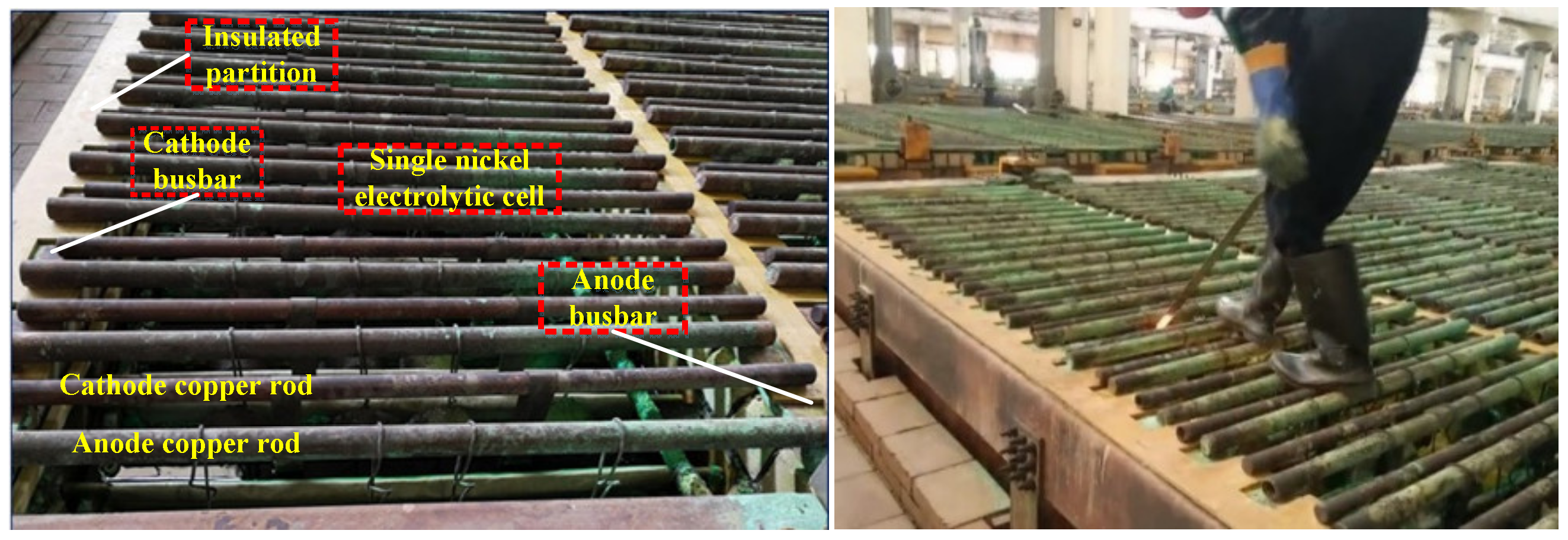
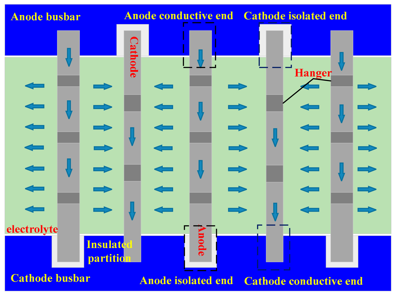
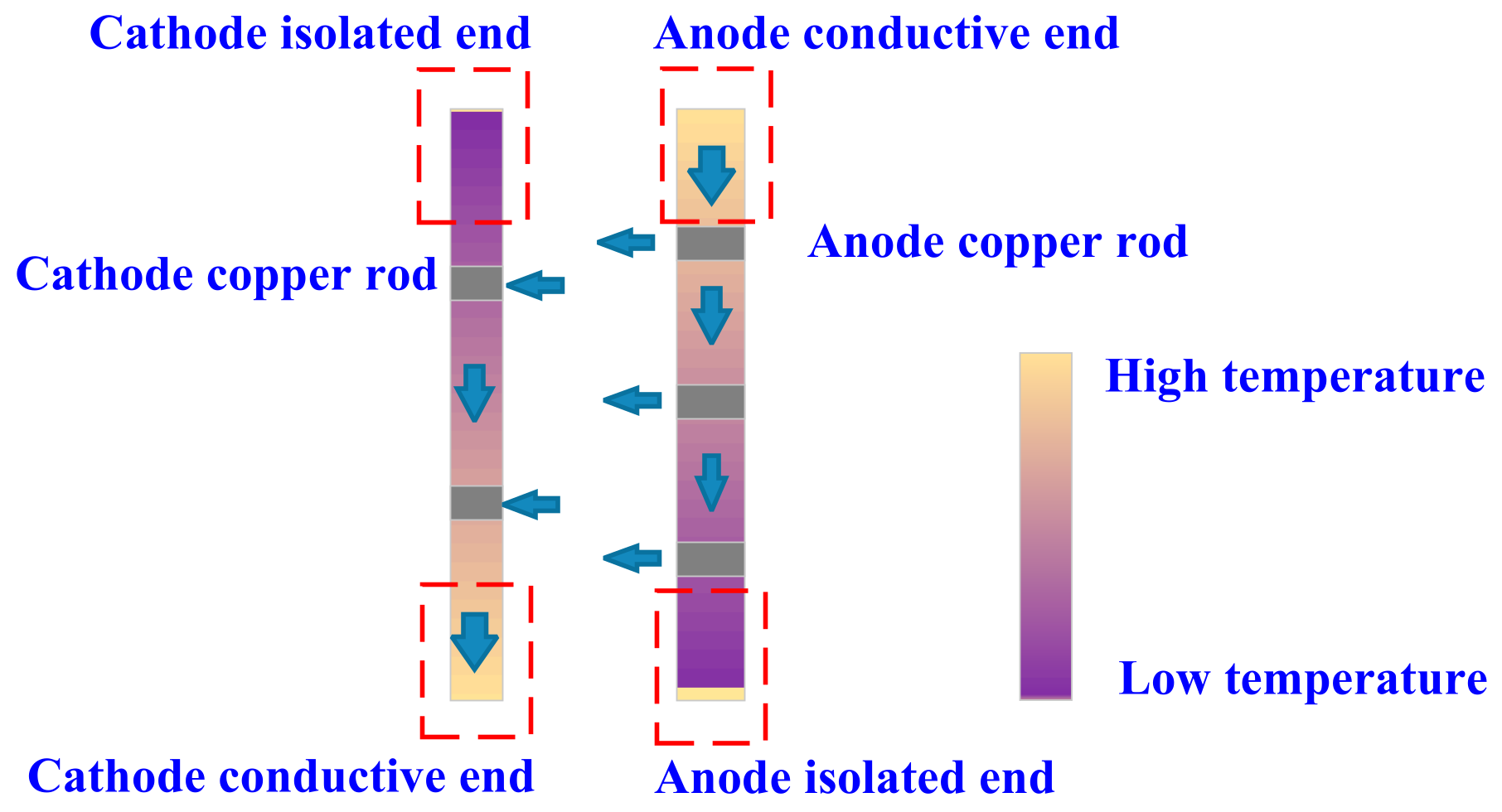
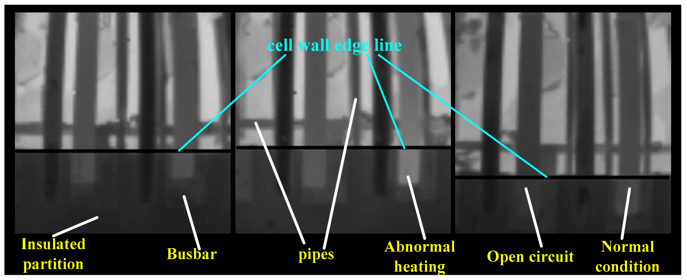
:1. Introduction
2. Solution Method
3. Infrared Image Segmentation
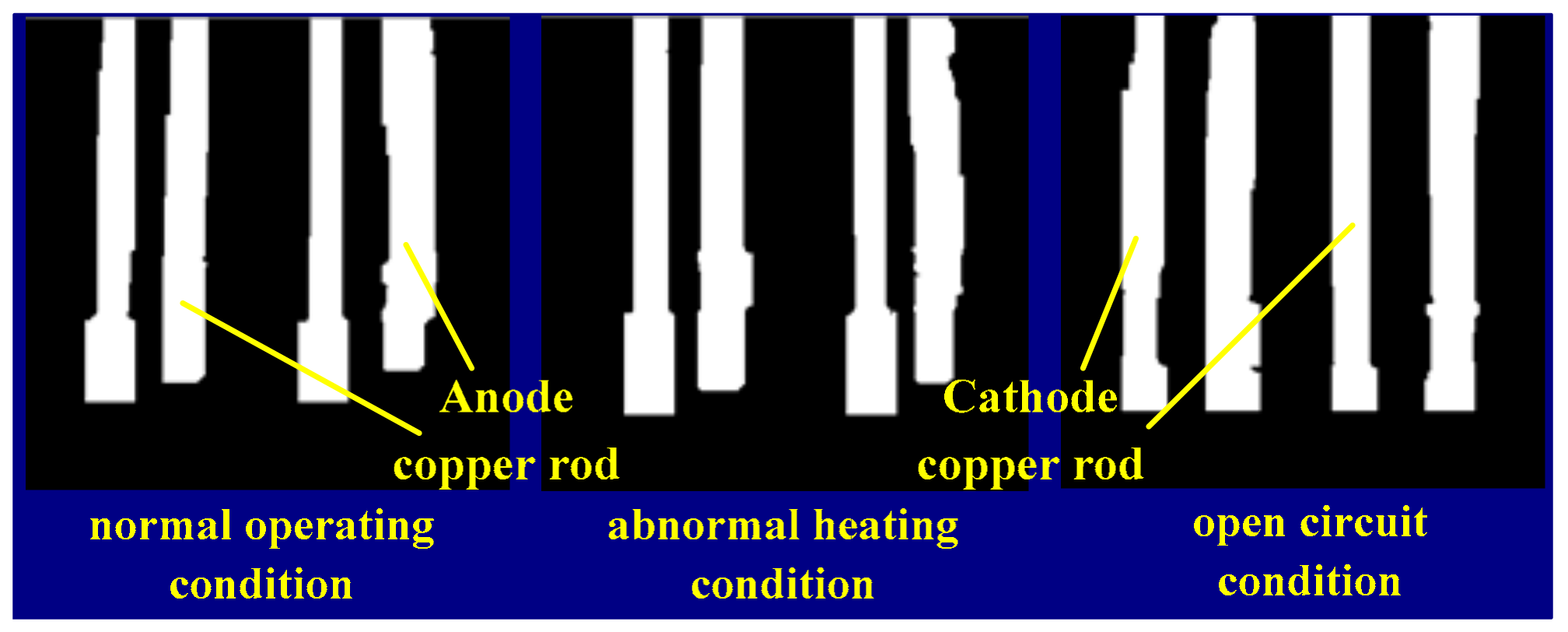
3.1. Copper Rod Segmentation Based on the Otsu Algorithm
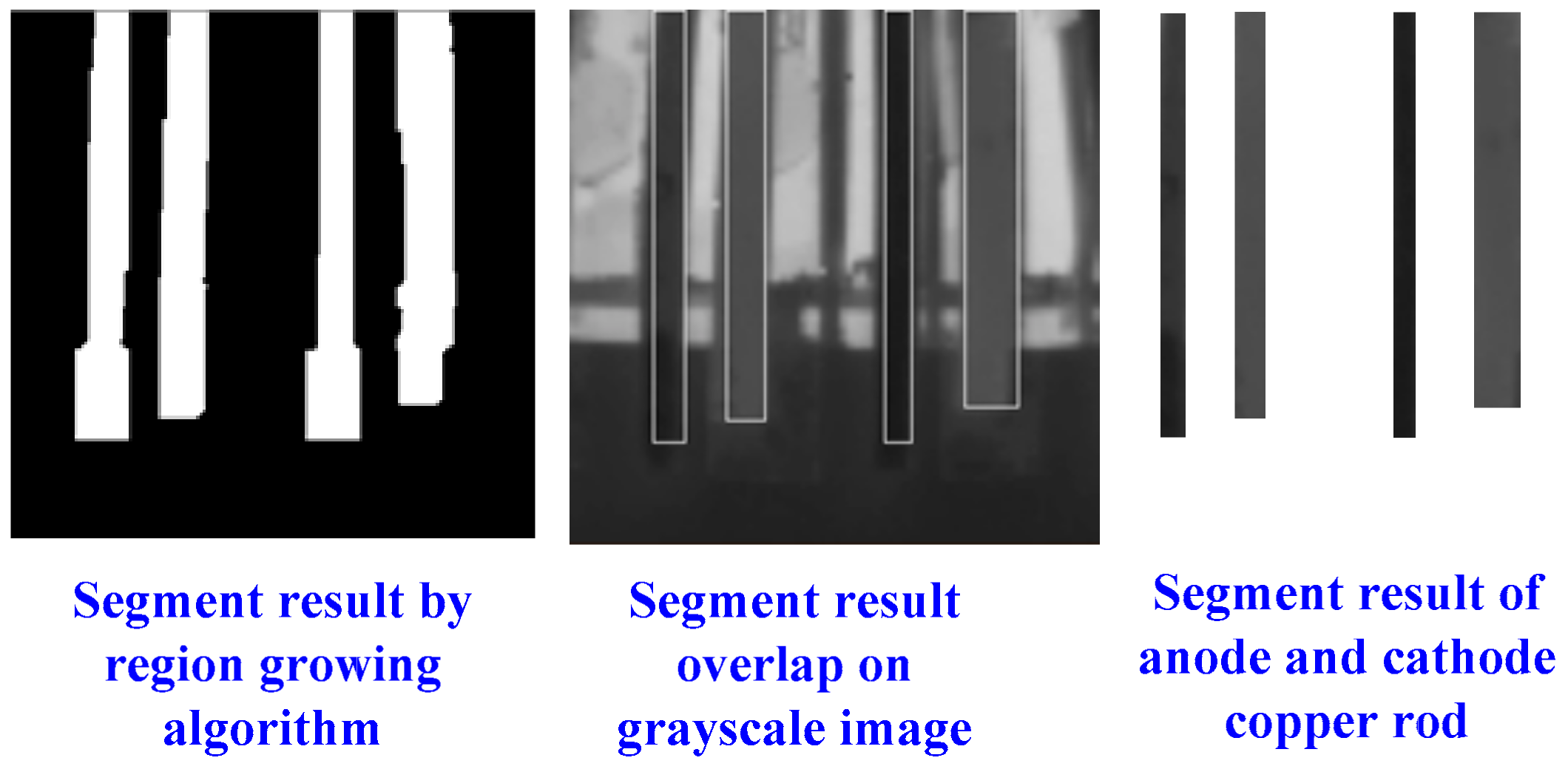
3.2. Copper Rod Segmentation Based on the Region Growing Algorithm
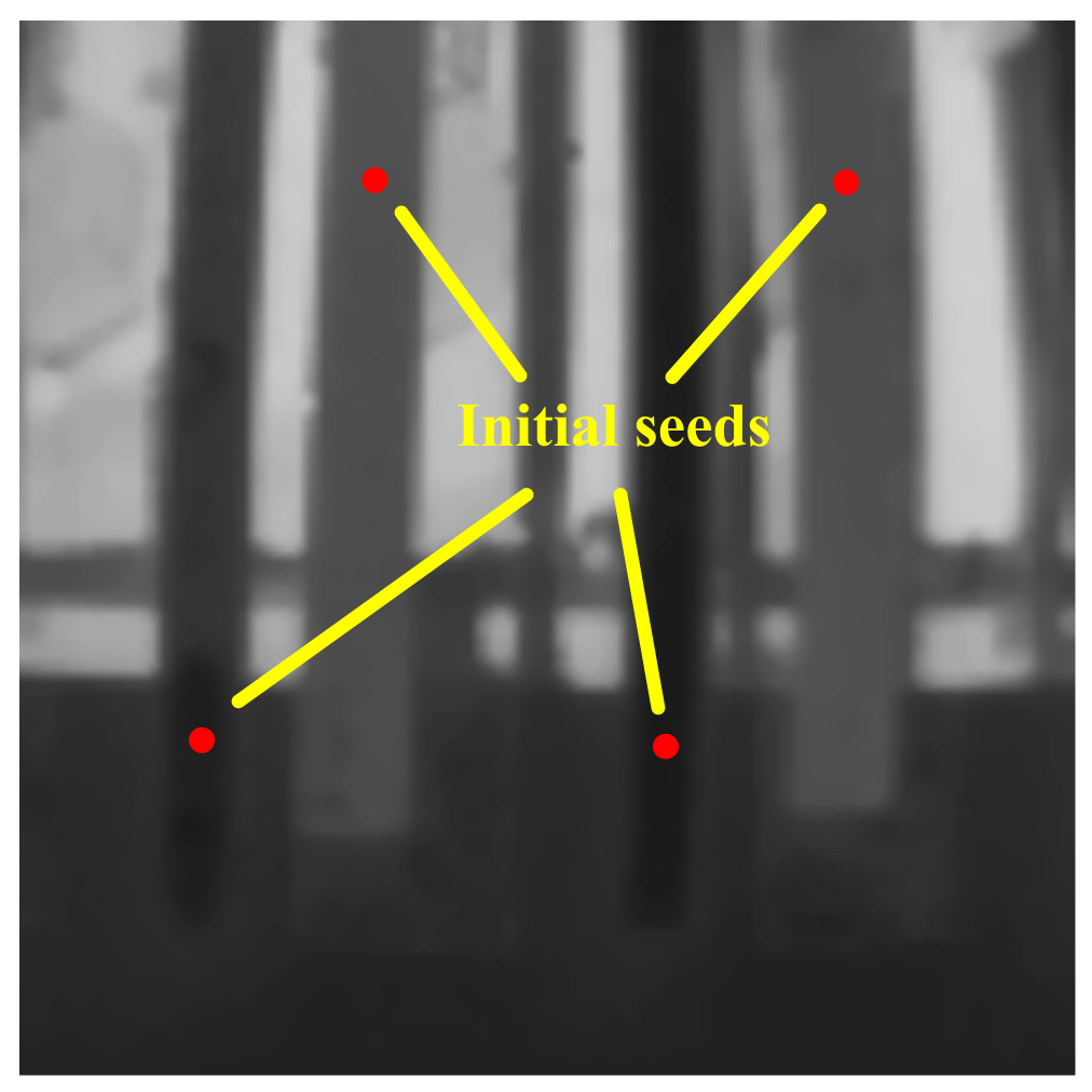
3.2.1. Selection of Initial Seeds
- (1)
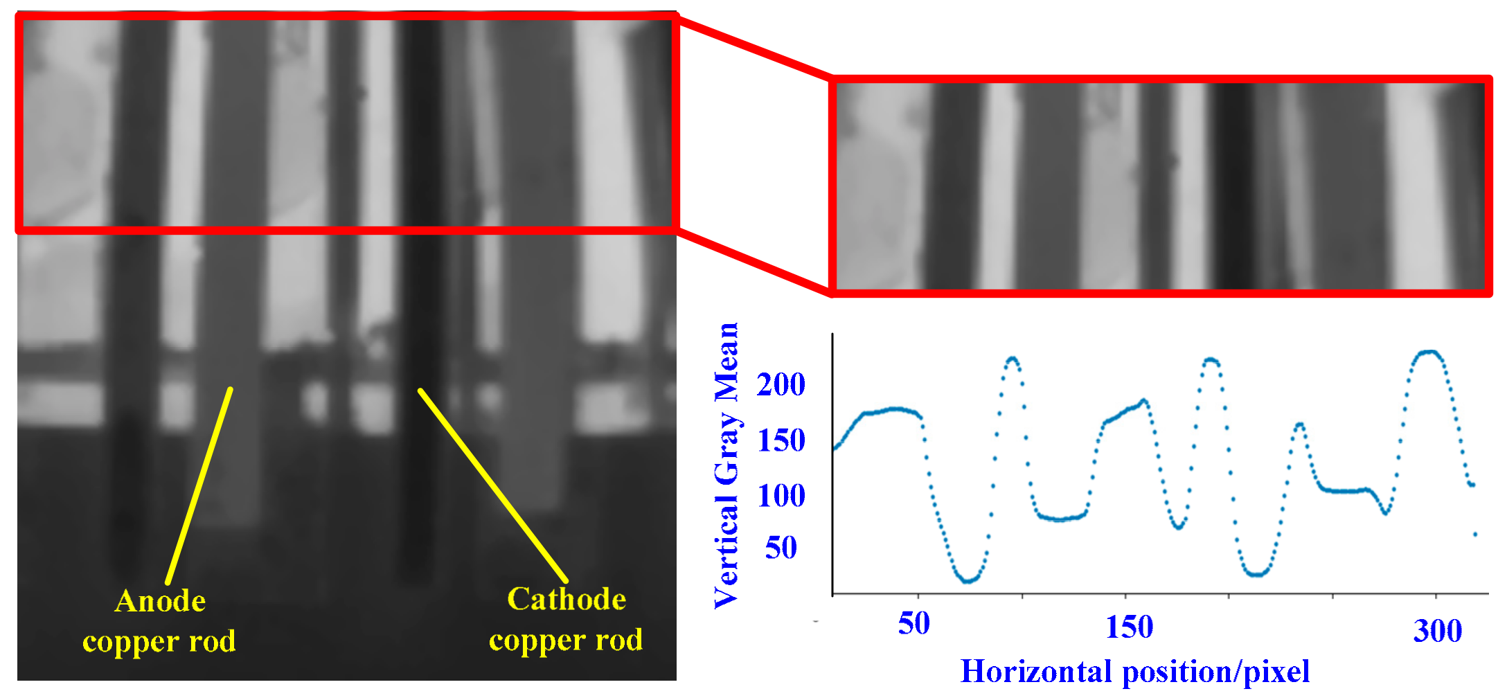
- Traverse all horizontal positions in the captured image, calculate the vertical gray mean at each position, and store it in array named verticalMean.
- (2)
- According to the width of the wide copper rod, set a variable named WinSlideSize for the sliding window length and initialize WinSlideSize to be equal to 20.
- (3)
- Traverse array verticalMean, enter step (4), and start to search for the position of the wide copper rod in the valley when the traversal results meet the following conditions:
- (4)
- Traverse array verticalMean from the index i, and calculate the variance in the sliding window named verticalMean [j:j+WinSlideSize]. When the variance is less than 5 for the first time, record the position as the start. When the variance is greater than 5 for the first time, the position is recorded as the end.
- (5)
- The positions of the initial seed for the wide copper rod are (start + end)/2, which are recorded in the array named WideRodPos. Then, return to step (3) and continue to traverse until all initial seeds of all wide copper rods are found.
3.2.2. Growing Criteria and Stopping Condition
Gray Difference Discrimination Method
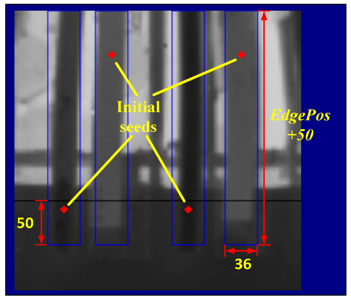
Limiting Growth Range Condition
3.3. Result of the Copper Rod Segmentation
4. Fault Identification
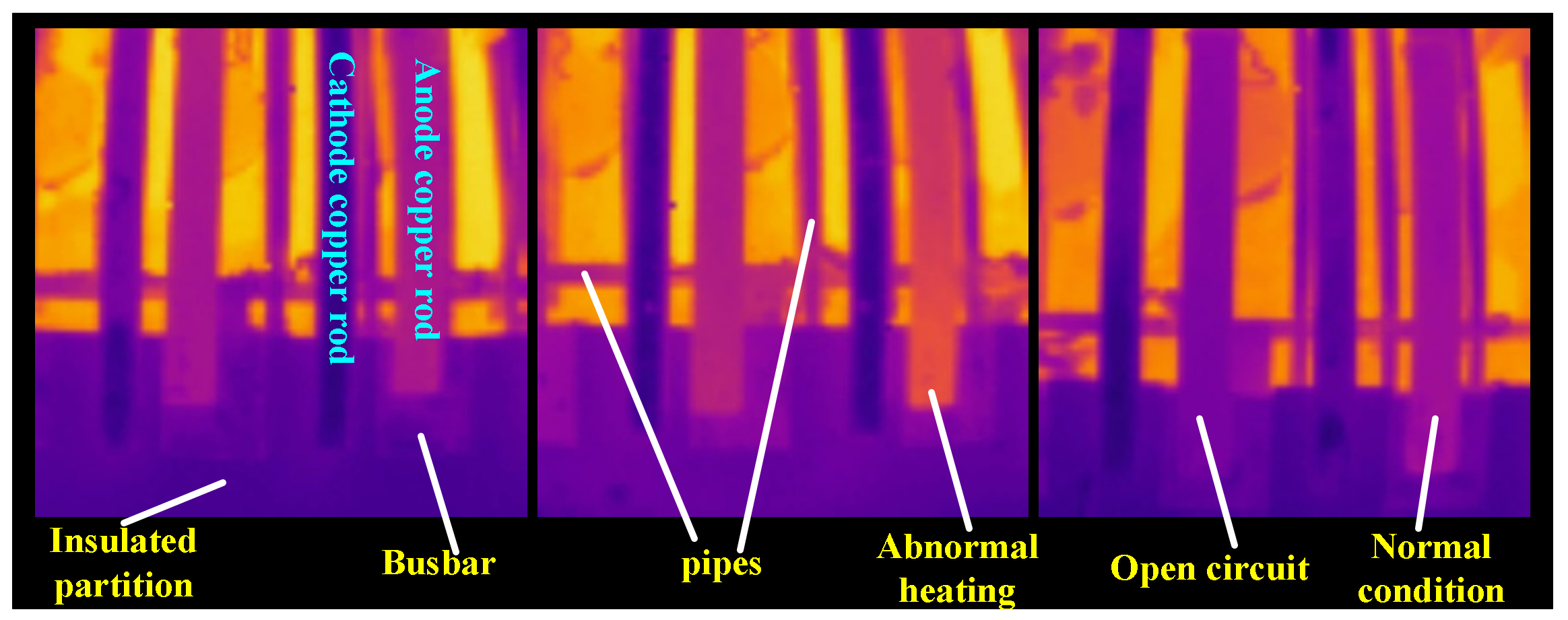
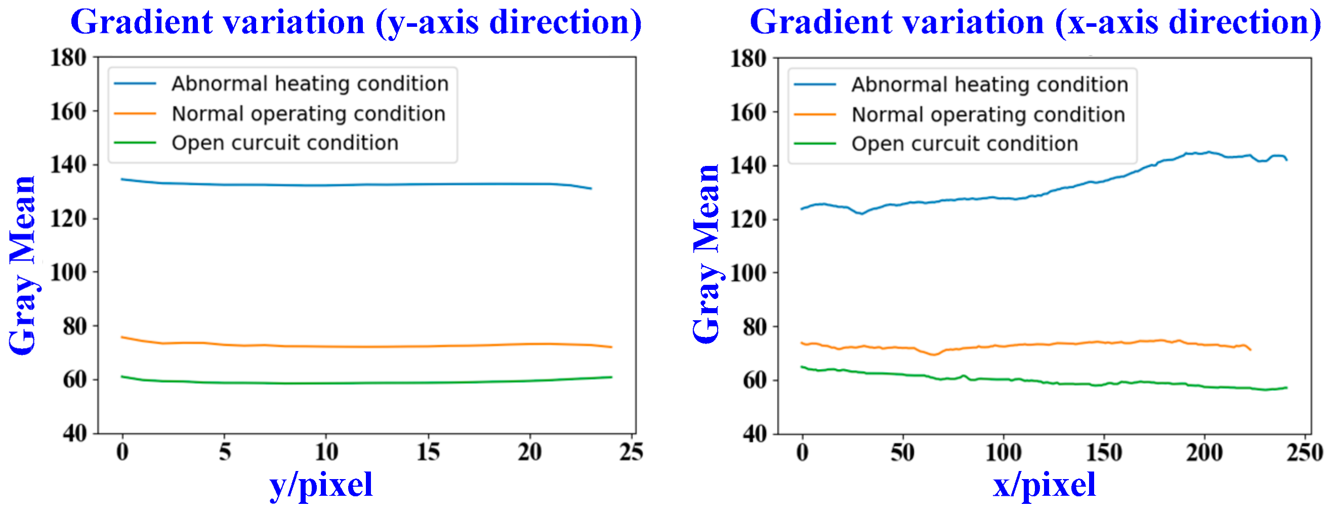
4.1. Infrared Feature Extraction
- (1)
- Gray mean (mean)
- (2)
- Gray standard deviation (std)
- (3)
- Mean gradient (G)
- (4)
- Deformation of Hu moments ( )
- (5)
- Gray difference between the target copper rod and the isolated end of the adjacent copper rod (D)
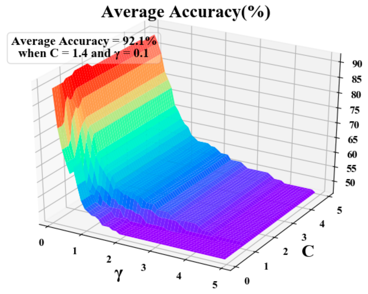
4.2. States Identification Based on Support Vector Machine
5. Conclusions
Author Contributions
Funding
Institutional Review Board Statement
Informed Consent Statement
Conflicts of Interest
References
- Wang, H.; Tie, J.; Xue, J.; Zhao, R. Investigation of Detection Method for Current Distribution in Ni-electrolyzer. Comput. Simul. 2014, 31, 245–249. [Google Scholar]
- Hu, X.; Li, Y.; Li, X.; Zhu, H.; Zhao, Y. Detection of Copper Electrolytic Short-Circuit Electrode by Convolution Neural Network and Infrared Thermography. In Proceedings of the 2018 China Automation Congress (CAC2018) Papers, Chinese Association of Automation, Xi’an, China, 30 November–2 December 2018. [Google Scholar]
- Zhao, R. Research on State Detection Method of Copper Electrolytic Refining Process Based on Infrared Images. Ph.D. Thesis, University of Science and Technology Beijing, Beijing, China, 2016. [Google Scholar]
- Jia, R.; Ma, X.; He, W. Infrared short-circuit detection for electrolytic copper refining. In Proceedings of the International Conference on Advanced Electronic Science and Technology, Shenzhen, China, 19–21 August 2016. [Google Scholar]
- Zhao, R.; Zhang, Y.; Tie, J.; Zhang, L.; Zhang, Z.; Guo, C. The Application of Infrared Thermography in the Current-distribution Measurement of Copper Electrolysis. Infrared Technol. 2015, 37, 981–985. [Google Scholar]
- Liang, L. Substation Infrared Image Recognition and Fault Diagnosis. Ph.D. Thesis, Xi’an University of Science and Technology, Xi’an, China, 2010. [Google Scholar]
- He, H.; Yao, J.; Jiang, Z.; Wang, X.X.; Li, W.W. Infrared thermal image detecting of high voltage insulator contamination grades based on Support Vector Machine. Autom. Electr. Power Syst. 2005, 29, 70–74. [Google Scholar]
- Fu, W.; Shi, F.; Wang, W.; Liu, Y.; Zhang, K.; Pei, S. Discriminating Threshold Selection Method and Diagnosis of Deteriorated Porcelain Insulator Based on Decision Tree. High Volt. Appar. 2019, 55, 149–154. [Google Scholar]
- Pei, S.; Liu, Y.; Chen, T.; Wu, J.; Liang, L. Infrared spectrum diagnosis method of deteriorated insulators based on BOA-SVM. Electr. Meas. Instrum. 2018, 55, 11–16. [Google Scholar]
- Deng, R.; Lin, Y.; Tang, W.; Gu, F.; Ball, A. Object-Based Thermal Image Segmentation for Fault Diagnosis of Reciprocating Compressors. Sensors 2020, 20, 3436. [Google Scholar] [CrossRef] [PubMed]
- Otsu, N. A Threshold Selection Method from Gray-Level Histograms. IEEE Trans. Syst. Man Cybern. 1979, 9, 62–66. [Google Scholar] [CrossRef] [Green Version]
- Chen, Q.; Zhao, L.; Lu, J.; Kuang, G.; Wang, N.; Jiang, Y. Modified two-dimensional Otsu image segmentation algorithm and fast realization. IET Image Process. 2012, 6, 426–433. [Google Scholar] [CrossRef]
- Zhang, P.; Kong, L. Wheel Defect Segmentation Based on Improved Otsu Method. In Proceedings of the 2018 IEEE 3rd International Conference on Signal and Image Processing (ICSIP), Shenzhen, China, 13–15 July 2018. [Google Scholar]
- Shi, J.; Lu, G.; Liu, J. Mentation based on modified region growing algorithm. Opt. Tech. 2017, 43, 381–384. [Google Scholar]
- Sanchez Hernandez, J.; Martinez Izquierdo, E.; Arquero Hidalgo, A. Improving Parameters Selection of a Seeded Region Growing Method for Multiband Image Segmentation. IEEE Lat. Am. Trans. 2015, 13, 843–849. [Google Scholar] [CrossRef] [Green Version]
- Shanmugam, C.; Sekaran, E.C. Optimal region growing and multi-kernel SVM for fault detection in electrical equipments using infrared thermography images. Int. J. Bus. Intell. Data Min. 2020, 17, 329–348. [Google Scholar] [CrossRef]
- Han, X.; Wang, X.; Leng, Y.; Zhou, W. A Plane Extraction Approach in Inverse Depth Images Based on Region-Growing. Sensors 2021, 21, 1141. [Google Scholar] [CrossRef] [PubMed]
- Sun, S.; Zhang, R. Region of Interest Extraction of Medical Image based on Improved Region Growing Algorithm. In Proceedings of the 2017 International Conference on Material Science, Energy and Environmental Engineering (MSEEE 2017), Xi’an, China, 26–28 August 2017. [Google Scholar]
- Xu, G.; Bu, Y.; Wang, L. A color image segmentation algorithm by integrating watershed with automatic seeded region growing and merging. Comput. Sci. Appl. 2011, 8200, 43. [Google Scholar]
- Hu, M.K. Visual Pattern Recognition by Moment Invariants. Inf. Theory IRE Trans. 1962, 8, 179–187. [Google Scholar]
- Ren, Y.; Yang, J.; Zhang, Q.; Guo, Z. Ship recognition based on Hu invariant moments and convolutional neural network for video surveillance. Multimed. Tools Appl. 2021, 80, 1343–1373. [Google Scholar] [CrossRef]
- Kondusov, D.V.; Sergeev, A.I.; Kondusova, V.B. Comparison of 3D Models Using Hu Moment Invariants. Russ. Eng. Res. 2020, 40, 570–574. [Google Scholar] [CrossRef]
- Zhao, J.; Wang, X. Vehicle-logo recognition based on modified HU invariant moments and SVM. Multimed. Tools Appl. 2019, 78, 75–97. [Google Scholar] [CrossRef]
- Hao, J.; Jia, C. Research on Fault Mode Diagnosis of Airborne Circuit Board Based on Infrared Images. Infrared Technol. 2019, 41, 273–278. [Google Scholar]
- Wu, Y.; Lu, Y. An intelligent machine vision system for detecting surface defects on packing boxes based on support vector machine. Meas. Control 2019, 52, 1102–1110. [Google Scholar] [CrossRef] [Green Version]
- Wang, Y.Q.; Tian, D.; Song, D.Y.; Zhang, L. Application of Improved Invariant Moments and SVM in the Recognition of Solar Cell Defects. In Applied Mechanics & Materials; Trans Tech Publications Ltd.: Freienbach, Switzerland, 2014; Volume 672, pp. 3–6. [Google Scholar]


| Mean | std | G | H1 | H2 | H3 | D | Label | |
|---|---|---|---|---|---|---|---|---|
| 1 | 100.8 | 7.1 | 0.77 | 4.87 | 9.79 | 19.5 | 65.37 | 0 |
| 2 | 100.58 | 7.17 | 0.79 | 4.89 | 9.83 | 19.57 | 68.52 | 0 |
| 3 | 83.55 | 10.73 | 1.45 | 4.76 | 9.58 | 21.35 | 48.69 | 0 |
| 4 | 73.97 | 10.07 | 1.29 | 4.57 | 9.2 | 19.09 | 40.56 | 1 |
| 5 | 76.82 | 2.05 | 0.51 | 4.59 | 9.23 | 21.15 | 42.61 | 1 |
| 6 | 74.84 | 2.07 | 0.69 | 4.79 | 9.66 | 23.34 | 46.33 | 1 |
| 7 | 48.01 | 3.62 | 1.05 | 4.03 | 8.11 | 18.83 | 15.48 | 2 |
| 8 | 45.05 | 2.45 | 0.61 | 3.97 | 7.99 | 20.11 | 14.23 | 2 |
| 9 | 44.9 | 2.42 | 0.62 | 3.92 | 8.01 | 20.26 | 14.64 | 2 |
| Conductive Conditions | Number of Test Samples | Correction | Misclassification | Accuracy | Total Accuracy |
|---|---|---|---|---|---|
| Abnormal heating condition | 10 | 7 | 3 | 70% | 90% |
| Normal operation condition | 10 | 10 | 0 | 100% | |
| Open circuit condition | 10 | 10 | 0 | 100% |
| Mean | std | G | H1 | H2 | H3 | D | |
|---|---|---|---|---|---|---|---|
| a | 83.55 | 10.73 | 1.45 | 4.76 | 9.58 | 21.35 | 48.69 |
| b | 100.58 | 7.17 | 0.79 | 4.89 | 9.83 | 19.57 | 68.52 |
| c | 73.97 | 10.07 | 1.29 | 4.57 | 9.2 | 19.09 | 40.56 |
Publisher’s Note: MDPI stays neutral with regard to jurisdictional claims in published maps and institutional affiliations. |
© 2022 by the authors. Licensee MDPI, Basel, Switzerland. This article is an open access article distributed under the terms and conditions of the Creative Commons Attribution (CC BY) license (https://creativecommons.org/licenses/by/4.0/).
Share and Cite
Sun, R.; Qin, G.; Li, G.; Hu, J.; Xiong, J.; Xu, H. Abnormal Conductive State Identification of the Copper Rod in a Nickel Electrolysis Procedure Based on Infrared Image Features and Position Characteristics. Appl. Sci. 2022, 12, 3691. https://doi.org/10.3390/app12073691
Sun R, Qin G, Li G, Hu J, Xiong J, Xu H. Abnormal Conductive State Identification of the Copper Rod in a Nickel Electrolysis Procedure Based on Infrared Image Features and Position Characteristics. Applied Sciences. 2022; 12(7):3691. https://doi.org/10.3390/app12073691
Chicago/Turabian StyleSun, Rui, Gang Qin, Gaibian Li, Jinbao Hu, Jingqi Xiong, and Huanwei Xu. 2022. "Abnormal Conductive State Identification of the Copper Rod in a Nickel Electrolysis Procedure Based on Infrared Image Features and Position Characteristics" Applied Sciences 12, no. 7: 3691. https://doi.org/10.3390/app12073691
APA StyleSun, R., Qin, G., Li, G., Hu, J., Xiong, J., & Xu, H. (2022). Abnormal Conductive State Identification of the Copper Rod in a Nickel Electrolysis Procedure Based on Infrared Image Features and Position Characteristics. Applied Sciences, 12(7), 3691. https://doi.org/10.3390/app12073691