Nonuniform Dual-Rate Extended Kalman-Filter-Based Sensor Fusion for Path-Following Control of a Holonomic Mobile Robot with Four Mecanum Wheels

Abstract

This paper presents an extended Kalman-filter-based sensor fusion approach, which enables path-following control of a holonomic mobile robot with four mecanum wheels. Output measurements of the mobile platform may be sensed at different rates: odometry and orientation data can be obtained at a fast rate, whereas position information may be generated at a slower rate. In addition, as a consequence of possible sensor failures or the use of lossy wireless sensor networks, the presence of the measurements may be nonuniform. These issues may degrade the path-following control performance. The consideration of a nonuniform dual-rate extended Kalman filter (NUDREKF) enables us to estimate fast-rate robot states from nonuniform, slow-rate measurements. Providing these estimations to the motion controller, a fast-rate control signal can be generated, reaching a satisfactory path-following behavior. The proposed NUDREKF is stated to represent any possible sampling pattern by means of a diagonal matrix, which is updated at a fast rate from the current, existing measurements. This fact results in a flexible formulation and a straightforward algorithmic implementation. A modified Pure Pursuit path-tracking algorithm is used, where the reference linear velocity is decomposed into Cartesian components, which are parameterized by a variable gain that depends on the distance to the target point. The proposed solution was evaluated using a realistic simulation model, developed with Simscape Multibody (Matlab/Simulink), of the four-mecanum-wheeled mobile platform. This model includes some of the nonlinearities present in a real vehicle, such as dead-zone, saturation, encoder resolution, and wheel sliding, and was validated by comparing real and simulated behavior. Comparison results reveal the superiority of the sensor fusion proposal under the presence of nonuniform, slow-rate measurements.

1. Introduction

A holonomic robot is a mobile robot where the number of controllable degrees of freedom (DOF) is the same as the number of total DOF—that is, the robot has no kinematic constraints [1]. In contrast, in a nonholonomic robot, the number of controllable DOF is less than the number of total DOF; thus, the robot may have one or more kinematic constraints. The main advantage of holonomic vehicles over nonholonomic vehicles is their ability to rotate and translate independently and simultaneously [2]—that is, to move in any direction immediately with any orientation, e.g., they can move sideways [3]. In other words, the holonomic vehicle is capable of omnidirectional movement [4]. Among others, mecanum wheels [5] are a special kind of wheel that can be installed on the robotic platform to achieve omnidirectional mobility. This feature of the mecanum-wheeled mobile platforms implies their use in a wide variety of fields [6]: military activities, industrial tasks, medical applications, educational environments, etc. However, they usually present some practical problems such as random wheel slippage and high-speed vibration, which may cause uncertain position errors and low efficiency [7].

In our work, a path-tracking application is developed for a holonomic robot equipped with four mecanum wheels. As no time constraints are required for the mobile platform to converge to and follow the path, the path-tracking application becomes a path-following motion control [8]. The Pure Pursuit path-tracking algorithm (see, e.g., [9]) is used in order to make the robotic platform follow a predefined path approximately. Modified versions of the algorithm can be found in literature. They introduce different approaches with the aim of improving the path-tracking behavior by minimizing oscillations and lateral error. For instance, in [10], the next position of the path is obtained by considering a factor (which is experimentally calculated) multiplied by the path error (the closest distance of the vehicle to the path); in [11], a derivative term is added to the desired curvature equation; in [12], multiple look ahead points along the target path are aggregated to form a spatially filtered steering command; in [13], the ideal vehicle speed is estimated from curvature information; in [14], fuzzy control techniques are applied to dynamically obtain the look ahead distance; in [15], linear interpolation for waypoints and tuning rules for the look ahead distance based on curvature and speed are proposed. In our case, the Pure Pursuit path-tacking algorithm computes reference linear velocities from position estimations provided by a Kalman filter. The novelty of our modified version lies in decomposing the reference linear velocity into Cartesian components, which are parameterized by a variable gain that depends on the distance to the target point.

The control solution proposed in this work uses the celebrated Kalman filter [16,17,18] via its extended version (see, e.g., [19]) in order to (i) estimate the nonlinear behavior of the mobile platform, provide not available (not measurable) variables, and reduce the possible process and measurement noise effect; (ii) fuse all the data provided by the different sensing devices (encoders and beacons) to be used in the control stage. These data may arrive to the filter at two different rates—that is, whereas rotational velocities and orientation may be sensed at a faster rate, position information is usually obtained at a slower rate. In addition, the possible occurrence of sensor failures or the use of lossy wireless sensor networks may make the presence of the measurements nonuniform. Not facing these facts in the control solution may degrade the path-following control performance. For this reason, a novel, nonuniform dual-rate extended Kalman filter (NUDREKF) is formulated in order to estimate fast-rate robot states from nonuniform, slow-rate measurements. Providing these estimations to the fast-rate motion controller, a proper control signal may be generated so as to achieve a satisfactory path-following behavior. The proposed NUDREKF introduces a flexible formulation based on the use of a diagonal matrix, which is updated at fast rate from the current, existing measurements, allowing any possible sampling pattern. This feature results in a straightforward algorithmic implementation.

Few works on (uniform) DREKF can be found in literature related to autonomous vehicle frameworks. For instance, the DREKF is used to better estimate unavailable system states in unmanned aerial vehicles [20] to manage uncertainty in an obstacle tracking application [21], to fuse output variables sensed at different rates in a self-driving vehicle [22] and in a two-wheeled mobile robot [23]. Nevertheless, to the best of the authors’ knowledge, no work is available coping with the problem of nonuniform measurements via the so-called NUDREKF. Only in [24,25] is this kind of filter used to deal with nonuniform and delayed measurements, but applied to numerical examples and case studies out of the autonomous vehicle field.

In order to authentically reproduce the expected real behavior of the robotic platform, Simscape Multibody is used in this work. This multibody modeling tool is an extension of Matlab/Simulink, where complex physical bodies and their interactions can be intuitively defined so as to realistically simulate system dynamics. In this way, the robot model can include nonlinearities present in the real vehicle such as dead-zone, saturation, encoder resolution, and wheel sliding. These model parameters can be previously validated by comparing real and simulated behavior. Simscape Multibody has been employed in some recent studies related to autonomous vehicle frameworks. For instance, in [26], an antilock braking system (ABS) control for a vehicle is simulated; in [27], a mathematical model needed for torque determination during robot locomotion is tested and validated; in [28], simulation results for even and uneven surfaces are compared for a tread robot; in [29], a mechatronic interface for mobile manipulators is developed; in [23], a path-following control for a two-wheeled mobile robot is simulated. To the best of authors’ knowledge, few works on the simulation of mecanum-wheeled mobile platforms via Simscape Multibody can be found in literature. Some examples may be [30,31], where different motion models including multiple contact forces for this kind of robot are simulated.

Summarizing, the main contributions of the work are as follows:

• Consideration of a NUDREKF, which enables us to generate fast-rate state estimates from nonuniform, slow-rate measurements to be supplied to the fast-rate motion controller in order to reach a satisfactory path-following behavior.
• Modification of the Pure Pursuit path-tacking algorithm to improve adaptability to the change in turning and curvature sections of paths.
• Development of a powerful simulation tool, which takes into account complex modeling aspects to realistically represent the mobile platform movement.

The paper is organized as follows. Section 2 describes the problem scenario and the proposed control solution. Section 3 is devoted to mathematical aspects such as kinematic modeling of the process (Section 3.1), formulation of the NUDREKF (Section 3.2), and presentation of the modified version of the Pure Pursuit algorithm (Section 3.3). Section 4 presents the simulation tool developed, focusing on the description of the nonlinear aspects of the model. Section 5 introduces the cases simulated and the results obtained, which are analyzed in detail via some cost indexes. Finally, some conclusions summarize the present work in Section 6.

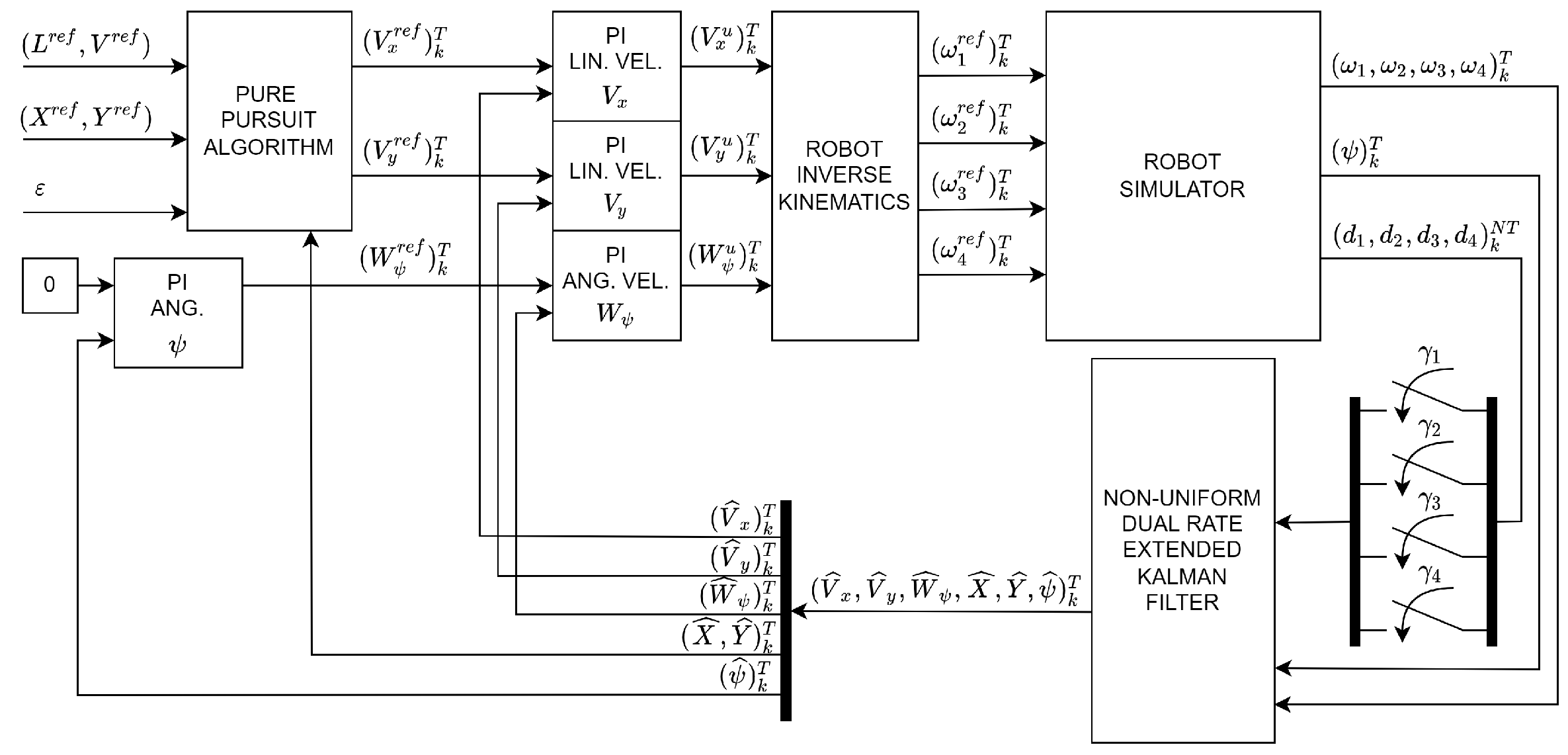
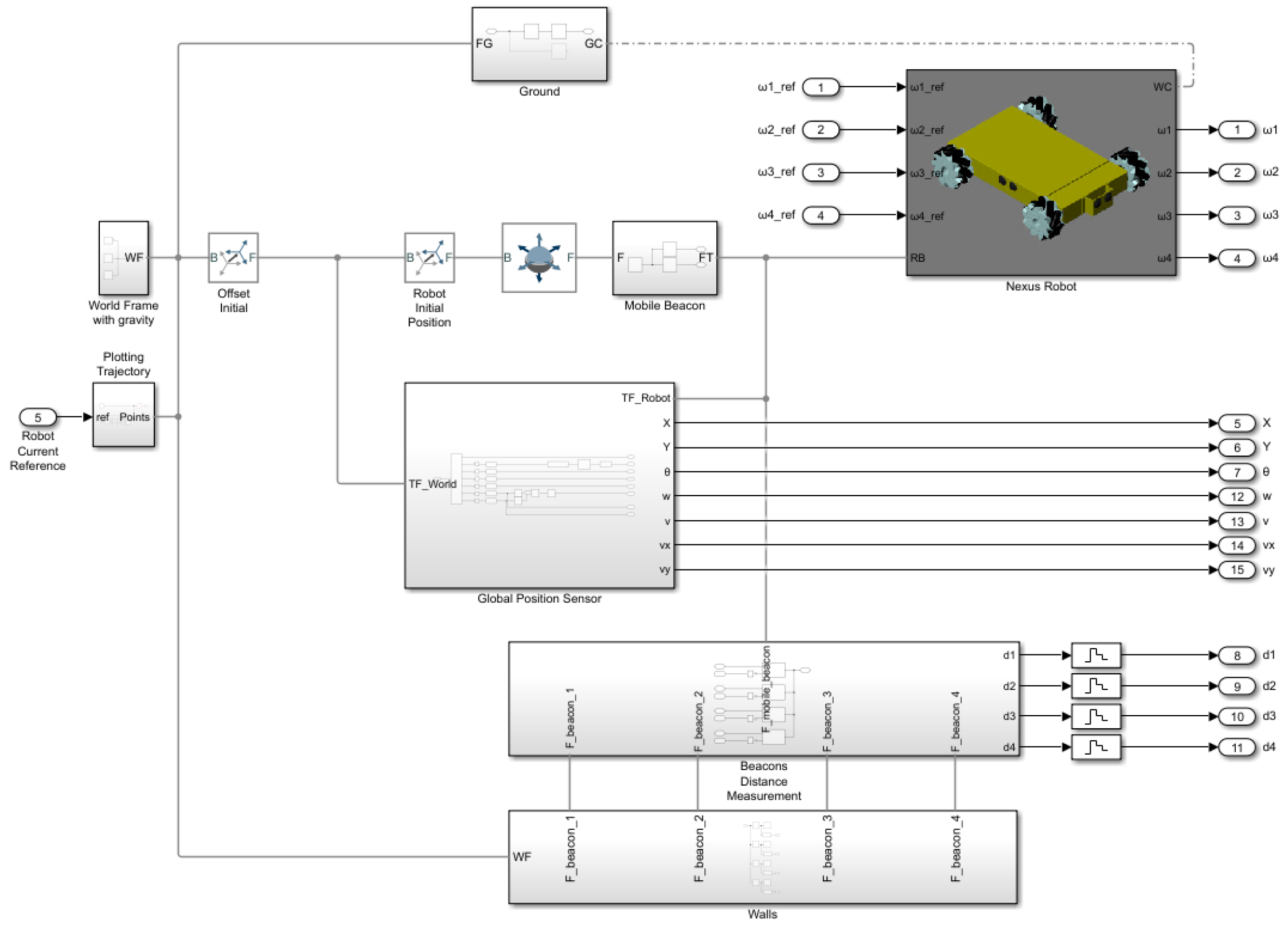
2. Problem Scenario

The overall control scheme is depicted in Figure 1, where two main parts can be distinguished:

• Robot simulator, which contains some complex vehicle modeling aspects as a result of using the features of the specialized Simscape Multibody simulation tool, and includes a dynamic proportional–integral (PI) controller for controlling the velocities of the wheels. More details can be found in Section 4.
• Control structure, which includes a path-tracking controller (in this case, the Pure Pursuit algorithm), PI controllers for angular orientation and linear and angular velocities, an inverse kinematics computation block, and a state estimator (in this case, the proposed NUDREKF).

The control structure generates the path reference based on waypoints and then generates the consequent actions to control the actuators. The main novelty of the NUDREKF concerning the DREKF [23] is the consideration of possible irregularities in the sampling period, such as loss of information from the sensors.

The control structure uses two different periods: T as the estimation and control period, and the sensing period for vehicle orientation and angular velocity; $NT$ as the vehicle position sensing period, where $N\in {\mathbb{N}}^{+}$ is the multiplicity between both periods. The position output will be more slowly sampled (at period $NT$) due to real hardware constraints in the beacon system. The beacon system also suffers from information losses denoted by ${\gamma }_i$. Let us, respectively, denote ${(.)}_k^T$ and ${(.)}_k^{NT}$ as a T-period and an $NT$-period signal or variable, where $k\in \mathbb{N}$ are iterations at the corresponding period. In more detail, the control structure works as follows:

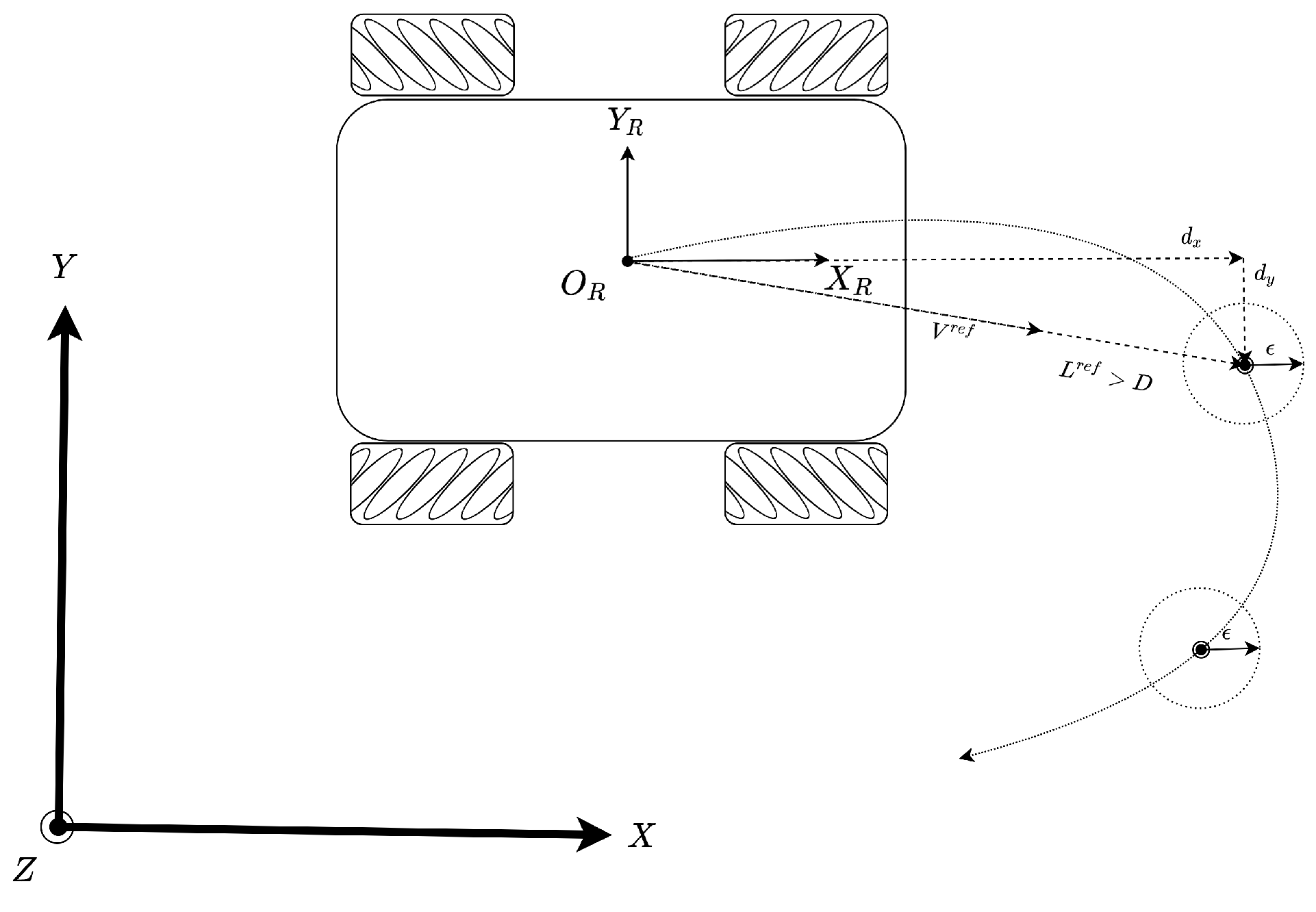
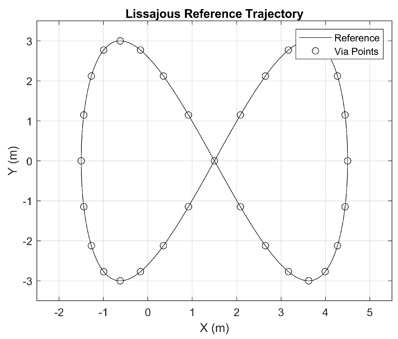
• At the current instant $kT$, from a set of waypoints and the current position estimation ${(\widehat{X},\widehat{Y})}_k^T$, the Pure Pursuit path-tracking algorithm [9] generates the reference linear velocities along the X-axis and Y-axis of the vehicle body, ${(V_x^{ref},V_y^{ref})}_k^T$. Other important parameters of the algorithm are the reference linear velocity $V^{ref}$, the look ahead distance $L^{ref}$, and the minimum distance $ϵ$ from the robot to the target point. More details about the Pure Pursuit algorithm will be given in Section 3.3.
• The reference linear velocities ${(V_x^{ref},V_y^{ref})}_k^T$ are injected to linear velocity PI controllers to generate the velocity control actions ${(V_x^u,V_y^u)}_k^T$. These PI controllers are used to reduce the negative effect that may cause dead-zones and possible external disturbances over the reference linear velocities. The vehicle inverse kinematics block transforms the velocity control actions ${(V_x^u,V_y^u,W_{\psi }^u)}_k^T$ into dynamic references ${({\omega }_1^{ref},{\omega }_2^{ref},{\omega }_3^{ref},{\omega }_4^{ref})}_k^T$.
• From these dynamic references ${({\omega }_1^{ref},{\omega }_2^{ref},{\omega }_3^{ref},{\omega }_4^{ref})}_k^T$, the internal dynamic PI controller (included in the robot simulator) computes the control signal to be applied to the vehicle. These control actions will be applied under Zero-Order Hold (ZOH) conditions.
• As a result, the robot outputs will be obtained. The vehicle is equipped with a virtual beacon. Four fixed beacons are additionally placed on the walls of the simulation environment, emulating a beacon-based indoor positioning system. The measurements ${(d_1,d_2,d_3,d_4)}_k^{NT}$ are the distances between the virtual mobile beacon and the four fixed beacons, which are located in a known place with respect to the world system of the simulator.
• Any vehicle output measurement ${({\omega }_1,{\omega }_2,{\omega }_3,{\omega }_4,\psi )}_k^T$, ${(d_1,d_2,d_3,d_4)}_k^{NT}$ may be disturbed by Gaussian noise, which will be created from a set of independent seeds in order to generate a reproducible pseudorandom noise. As a consequence, the experiments developed with the simulator will be reproducible under the same conditions.
• In addition, each of the position distances ${(d_1,d_2,d_3,d_4)}_k^{NT}$ may be individually lost according to a pseudorandom uniform probability distribution with loss probability $\mathit{P}$. When a position distance $d_i(i=1,\dots ,4)$ is lost, ${\gamma }_i=0$; otherwise, ${\gamma }_i=1$.
• The system state estimate ${({\widehat{V}}_x,{\widehat{V}}_y,{\widehat{W}}_{\psi },\widehat{X},\widehat{Y},\widehat{\psi })}_k^T$ is computed via the NUDREKF. The prediction step is generated at period T from the odometry measurements ${({\omega }_1,{\omega }_2,{\omega }_3,{\omega }_4)}_k^T$. The correction step is also obtained at period T, but from data sensed at the two different periods—that is, ${(\psi )}_k^T$ and ${(d_1,d_2,d_3,d_4)}_k^{NT}$. More details about the proposed NUDREKF can be found in Section 3.2.

3. Mathematical Foundations

In this section, the mathematical aspects of the work are presented. First, the model of the four-mecanum-wheeled mobile platform is stated. Second, the formulation of the NUDREKF is presented. Finally, the modified Pure Pursuit path-tracking algorithm is introduced.

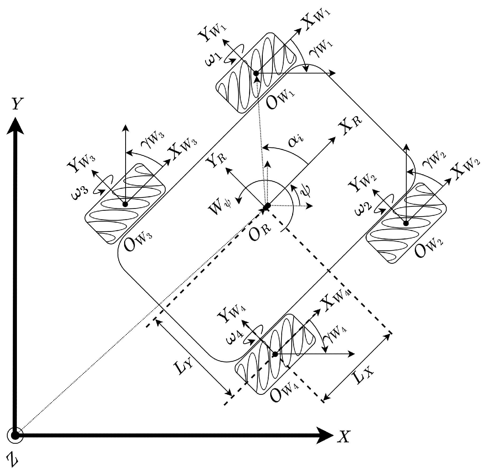
3.1. Kinematic and Dynamic Vehicle Modeling

The kinematic model represents the vehicle velocity evolution in a fixed inertial frame (see in Figure 2). A discrete-time version of the model at period T can be deduced as follows. A detailed description of the kinematic modeling can be found in [32,33]:

$$\begin{array}{cc}\hfill {\left(V_x\right)}_k^T& = \left({\left({\omega }_1\right)}_k^T+{\left({\omega }_2\right)}_k^T+{\left({\omega }_3\right)}_k^T+{\left({\omega }_4\right)}_k^T\right)·\frac{R}{4}\hfill \\ \hfill {\left(V_y\right)}_k^T& = \left(-{\left({\omega }_1\right)}_k^T+{\left({\omega }_2\right)}_k^T+{\left({\omega }_3\right)}_k^T-{\left({\omega }_4\right)}_k^T\right)·\frac{R}{4}\hfill \\ \hfill {\left(W_{\psi }\right)}_k^T& = \left(-{\left({\omega }_1\right)}_k^T+{\left({\omega }_2\right)}_k^T-{\left({\omega }_3\right)}_k^T+{\left({\omega }_4\right)}_k^T\right)·\frac{R}{4·(L_x+L_y)}\hfill \\ \hfill V_k^T& =\sqrt{{({\left(V_x\right)}_k^T)}^2+{({\left(V_y\right)}_k^T)}^2}\hfill \\ \hfill X_k^T& =X_{k-1}^T+V_k^{T}Tcos({\psi }_{k-1}^T+{\left(W_{\psi }\right)}_k^{T}T)\hfill \\ \hfill Y_k^T& =Y_{k-1}^T+V_k^{T}Tsin({\psi }_{k-1}^T+{\left(W_{\psi }\right)}_k^{T}T)\hfill \\ \hfill {\psi }_k^T& ={\psi }_{k-1}^T+{\left(W_{\psi }\right)}_k^{T}T\hfill \end{array}$$

(1)

where R is the radius of the wheel, and $L_x$ and $L_y$ are, respectively, the distance between the center of the wheels and the center of the robot along the longitudinal and lateral body axis of the robot. The linear and angular velocity control actions are transformed into reference rotational velocities by means of the inverse kinematic model:

$$\begin{array}{c}\hfill {({\omega }_1^{ref})}_k^T=\frac{1}{R}·({\left(V_x^u\right)}_k^T-{\left(V_y^u\right)}_k^T-(L_x+L_y)·{(W_{\psi }^u)}_k^T)\\ \hfill {({\omega }_2^{ref})}_k^T=\frac{1}{R}·({\left(V_x^u\right)}_k^T+{\left(V_y^u\right)}_k^T+(L_x+L_y)·{(W_{\psi }^u)}_k^T)\\ \hfill {({\omega }_3^{ref})}_k^T=\frac{1}{R}·({\left(V_x^u\right)}_k^T+{\left(V_y^u\right)}_k^T-(L_x+L_y)·{(W_{\psi }^u)}_k^T)\\ \hfill {({\omega }_4^{ref})}_k^T=\frac{1}{R}·({\left(V_x^u\right)}_k^T-{\left(V_y^u\right)}_k^T+(L_x+L_y)·{(W_{\psi }^u)}_k^T)\end{array}$$

(2)

In this work, although the mobile platform has 3 DOF, only two of them will be used in order to reach any 2D point (i.e., lateral and longitudinal movement). Then, the reference orientation is set to 0 (i.e., ${\left({\psi }^{ref}\right)}_k^T=0)$.

3.2. Non-Uniform Dual-Rate Extended Kalman Filter (NUDREKF)

In this section, the NUDREKF is stated. Its formulation is based on a well-known theory about nonuniform, multirate, sampled-data system modeling [34,35,36], which will be revisited in the next subsection.

3.2.1. Nonuniform, Multirate, Sampled-Data System Modeling

First of all, let us consider a continuous time-invariant linear state-space plant model:

$$\begin{array}{c}\hfill \dot{x}\left(t\right)=A·x\left(t\right)+B·u\left(t\right)\\ \hfill y\left(t\right)=C·x\left(t\right)+D·u\left(t\right)\end{array}$$

(3)

where $t\in {\mathbb{R}}^{+}$, $x\in {\mathbb{R}}^n$ is the state vector, $u\in {\mathbb{R}}^m$ is the control input vector, and $y\in {\mathbb{R}}^p$ is the output vector. In consequence, the state transition matrix $A\in {\mathbb{R}}^{n\times n}$, the input matrix $B\in {\mathbb{R}}^{n\times m}$, the output matrix $C\in {\mathbb{R}}^{p\times n}$, and the feedthrough (or feedforward) $D\in {\mathbb{R}}^{p\times m}$.

Assuming a periodic sampling T (i.e., $t=k·T,k\in \mathbb{N}$), a discrete-time-invariant, linear, state-space plant model under ZOH conditions yields

$$\begin{array}{cc}\hfill x_{k+1}^T& =A_{SR}·x_k^T+B_{SR}·u_k^T\hfill \\ \hfill y_k^T& =C_{SR}·x_k^T+D_{SR}·u_k^T\hfill \end{array}$$

(4)

where

$$\begin{array}{c}\hfill A_{SR}=e^{A·T}\\ \hfill B_{SR}={\int }_0^T{e}^{As}Bds\\ \hfill C_{SR}=C\\ \hfill D_{SR}=D\end{array}$$

An example of sampling scheme for a nonuniform, multirate, sampled-data multiple-input multiple-output (MIMO) system is depicted in Figure 3.

To represent the different sampling times, two diagonal matrices of dimensions $m\times m$ and $p\times p$ can be used as follows:

$$\begin{array}{cc}\hfill {\left({\mathsf{\Delta }}^u\right)}_k^T& \equiv diag\left\{{\left[{\delta }^u\right]}_k^T\left(i\right),i=1,2,\dots ,m\right\}\hfill \\ \hfill {\left({\mathsf{\Delta }}^y\right)}_k^T& \equiv diag\left\{{\left[{\delta }^y\right]}_k^T\left(i\right),i=1,2,\dots ,p\right\}\hfill \\ \hfill [{\delta }^u{]}_k^T\left(i\right)& \equiv \left\{\begin{array}{cc}1,& \mathrm{when}\mathrm{there}\mathrm{is}\mathrm{a}\mathrm{sample}\\ 0,& \mathrm{otherwise}\end{array}\right.\hfill \\ \hfill [{\delta }^y{]}_k^T\left(i\right)& \equiv \left\{\begin{array}{cc}1,& \mathrm{when}\mathrm{there}\mathrm{is}\mathrm{a}\mathrm{sample}\\ 0,& \mathrm{otherwise}\end{array}\right.\hfill \end{array}$$

(5)

Following the principles developed in [37,38], a nonuniform, multirate, sampled-data system can be expressed as two discrete time systems, one of them representing the plant and another one representing the input-hold process

$${\overline{x}}_{k+1}^T={\left(A_{MR}\right)}_k^T·{\overline{x}}_k^T+{\left(B_{MR}\right)}_k^T·u_k^T$$

(6)

where ${\left[{\overline{x}}_k^T\right]}^{\top }\equiv \left[\begin{array}{cc}{\left[x_k^T\right]}^{\top }& {\left[{\left({\nu }^u\right)}_k^T\right]}^{\top }\end{array}\right]\in R^{n+m}$ is an extended state vector and ${\left({\nu }^u\right)}_k^T$ is the held input. Note that ${[·]}^{\top }$ denotes the transpose function. The matrices ${\left(A_{MR}\right)}_k^T,{\left(B_{MR}\right)}_k^T$ are defined as

$$\begin{array}{cc}\hfill {\left(A_{MR}\right)}_k^T& =\left[\begin{array}{cc}{A}_{SR}& B_{SR}\left(T\right)·(I-{\left({\mathsf{\Delta }}^u\right)}_k^T)\\ 0& I-{\left({\mathsf{\Delta }}^u\right)}_k^T\end{array}\right]\hfill \\ \hfill {\left(B_{MR}\right)}_k^T& =\left[\begin{array}{c}{B}_{SR}\left(T\right) · {\left({\mathsf{\Delta }}^u\right)}_k^T\\ {\left({\mathsf{\Delta }}^u\right)}_k^T\end{array}\right]\hfill \end{array}$$

(7)

being $B_{SR}\left(T\right)={\int }_0^T{e}^{A·(T-s)}Bds$.

These multirate matrices can be easily obtained as the product of two independent matrices: the first one corresponds to the single-rate system, and the second one to the nonuniform multirate sampling procedure. So, we have

$$\begin{array}{cc}\hfill {\left[\begin{array}{c}x\\ u\end{array}\right]}_{k+1}^T& ={\left(H_{SRD}\right)}_k^T·{\left(H_{MRS}\right)}_k^T·{\left[\begin{array}{c}x\\ {\nu }^u\\ u\end{array}\right]}_k^T\hfill \\ \hfill & =\left[\begin{array}{cc}{A}_{SR}& B_{SR}\left(T\right)\\ 0& I\end{array}\right]·\left[\begin{array}{ccc}I& 0& 0\\ 0& I-{\left({\mathsf{\Delta }}^u\right)}_k^T& {\left({\mathsf{\Delta }}^u\right)}_k^T\end{array}\right]·{\left[\begin{array}{c}x\\ {\nu }^u\\ u\end{array}\right]}_k^T\hfill \end{array}$$

(8)

If a similar reasoning is additionally applied to output signals, a compact, nonuniform, multirate, discrete model can be obtained as follows:

$${\left[\begin{array}{c}{x}_{k+1}\\ {\nu }_{k+1}^u\\ {\nu }_{k+1}^y\\ u_k\\ y_k\end{array}\right]}^T=\left[\begin{array}{cccc}{A}_{SR}& B_{SR}\left(T\right)·(I-{\left({\mathsf{\Delta }}^u\right)}_k^T)& 0& B_{SR}\left(T\right)·{\left({\mathsf{\Delta }}^u\right)}_k^T\\ 0& I-{\left({\mathsf{\Delta }}^u\right)}_k^T& 0& {\left({\mathsf{\Delta }}^u\right)}_k^T\\ {\left({\mathsf{\Delta }}^y\right)}_k^T·C_{SR}& 0& I-{\left({\mathsf{\Delta }}^u\right)}_k^T& {\left({\mathsf{\Delta }}^y\right)}_k^T·D_{SR}·{\left({\mathsf{\Delta }}^u\right)}_k^T\\ 0& 0& 0& I\\ {\left({\mathsf{\Delta }}^y\right)}_k^T·C_{SR}& {\left({\mathsf{\Delta }}^y\right)}_k^T·D_{SR}·(I-{\left({\mathsf{\Delta }}^u\right)}_k^T)& I-{\left({\mathsf{\Delta }}^u\right)}_k^T& {\left({\mathsf{\Delta }}^y\right)}_k^T·D_{SR}·{\left({\mathsf{\Delta }}^u\right)}_k^T\end{array}\right]{\left[\begin{array}{c}x\\ {\nu }^u\\ {\nu }^y\\ u\end{array}\right]}_k^T$$

(9)

where, now,

$$\begin{array}{cc}\hfill {\left(A_{MR}\right)}_k^T& =\left[\begin{array}{ccc}{A}_{SR}& B_{SR}\left(T\right)·(I-{\left({\mathsf{\Delta }}^u\right)}_k^T)& 0\\ 0& I-{\left({\mathsf{\Delta }}^u\right)}_k^T& 0\\ {\left({\mathsf{\Delta }}^y\right)}_k^T·C_{SR}& 0& I-{\left({\mathsf{\Delta }}^y\right)}_k^T\end{array}\right]\hfill \\ \hfill {\left(B_{MR}\right)}_k^T& =\left[\begin{array}{c}{B}_{SR}\left(T\right)·{\left({\mathsf{\Delta }}^u\right)}_k^T\\ {\left({\mathsf{\Delta }}^u\right)}_k^T\\ {\left({\mathsf{\Delta }}^y\right)}_k^T·D_{SR}\end{array}\right]\hfill \\ \hfill {\left(C_{MR}\right)}_k^T& =\left[\begin{array}{ccc}{\left({\mathsf{\Delta }}^y\right)}_k^T·C_{SR}& {\left({\mathsf{\Delta }}^y\right)}_k^T·D_{SR}·(I-{\left({\mathsf{\Delta }}^u\right)}_k^T)& I-{\left({\mathsf{\Delta }}^y\right)}_k^T\end{array}\right]\hfill \\ \hfill {\left(D_{MR}\right)}_k^T& =\left[{\mathsf{\Delta }}_k^y·D_{SR}·{\mathsf{\Delta }}_k^u\right]\hfill \end{array}$$

(10)

The proposed NUDREKF-based control structure considers nonuniform, dual-rate, sampled-data system outputs and fast-rate inputs to the plant. Then, from the previous formulation, we will have

$${\left[\begin{array}{c}x\\ {\nu }^y\end{array}\right]}_{k+1}^T=\left[\begin{array}{cc}{A}_{SR}& 0\\ {\left({\mathsf{\Delta }}^y\right)}_k^T·C_{SR}& I-{\left({\mathsf{\Delta }}^y\right)}_k^T\end{array}\right]{\left[\begin{array}{c}x\\ {\nu }^y\end{array}\right]}_k^T+\left[\begin{array}{c}{B}_{SR}\left(T\right)\\ {\left({\mathsf{\Delta }}^y\right)}_k^T·D_{SR}\end{array}\right]u_k^T$$

(11)

$$y_k^T=\left[\begin{array}{cc}{\left({\mathsf{\Delta }}^y\right)}_k^T·C_{SR}& I-{\left({\mathsf{\Delta }}^y\right)}_k^T\end{array}\right]{\left[\begin{array}{c}x\\ {\nu }^y\end{array}\right]}_k^T+\left[{\left({\mathsf{\Delta }}^y\right)}_k^T·D_{SR}\right]u_k^T$$

(12)

being

$$\begin{array}{cc}\hfill {\left(A_{MR}\right)}_k^T& =\left[\begin{array}{cc}{A}_{SR}& 0\\ {\left({\mathsf{\Delta }}^y\right)}_k^T·C_{SR}& I-{\left({\mathsf{\Delta }}^y\right)}_k^T\end{array}\right]\hfill \\ \hfill {\left(B_{MR}\right)}_k^T& =\left[\begin{array}{c}{B}_{SR}\left(T\right)\\ {\left({\mathsf{\Delta }}^y\right)}_k^T·D_{SR}\end{array}\right]\hfill \\ \hfill {\left(C_{MR}\right)}_k^T& =\left[\begin{array}{cc}{\left({\mathsf{\Delta }}^y\right)}_k^T·C_{SR}& I-{\left({\mathsf{\Delta }}^y\right)}_k^T\end{array}\right]\hfill \\ \hfill {\left(D_{MR}\right)}_k^T& =\left[{\left({\mathsf{\Delta }}^y\right)}_k^T·D_{SR}\right]\hfill \end{array}$$

(13)

3.2.2. Formulation of the NUDREKF

The previous reasoning can be applied to the well-known Extended Kalman Filter equations [19]:

$$\begin{array}{cc}\hfill {\xi }_{k+1}^T& =f\left({\xi }_k^T\right)+h\left({\xi }_k^T\right)·u_k^T\hfill \\ \hfill z_k^T& =g\left({\xi }_k^T\right)+{\eta }_k^T\hfill \end{array}$$

(14)

where ${\xi }_k^T$ is the vehicle state, which is composed of ${\left[{(V_x,V_y,W_{\psi },X,Y,\psi )}_k^T\right]}^{\top }$; the control signal is $u_k^T={\left[{({\omega }_1,{\omega }_2,{\omega }_3,{\omega }_4)}_k^T\right]}^{\top }$; ${\eta }_k^T$ is a possible measurement noise, which is assumed to be zero mean multivariate Gaussian noise with covariance $R_k^T$; and the output is $z_k^T={\left[{(V_x,V_y,W_{\psi },\psi ,{\gamma }_1·d_1,{\gamma }_2·d_2,{\gamma }_3·d_3,{\gamma }_4·d_4)}_k^T\right]}^{\top }$, being $d_i\ne 0,(i=1\dots 4)$ at times $k=NT$ and ${\gamma }_i=1$ if no measurement loss is produced (otherwise, ${\gamma }_i=0$).

The nonlinear functions f and g can be linearized as follows:

$$\begin{array}{cc}\hfill f\left({\xi }_k^T\right)& \approx f\left({\widehat{\xi }}_k^T\right)+{\left.\frac{\partial f}{\partial \xi }\right|}_{{\widehat{\xi }}_k^T}·\left({\xi }_k^T-{\widehat{\xi }}_k^T\right)\hfill \\ \hfill g\left({\xi }_k^T\right)& \approx g\left({\widehat{\xi }}_{k|k-1}^T\right)+{\left.\frac{\partial g}{\partial \xi }\right|}_{{\widehat{\xi }}_{k|k-1}^T}·\left({\xi }_k^T-{\widehat{\xi }}_{k|k-1}^T\right)\hfill \end{array}$$

(15)

where, as usual, the notation ${\widehat{\xi }}_{k|k-1}^T$ means the state estimated for the instant k from the instant $k-1$. If the previous nonuniform multirate modeling is applied to the linearized model, it yields

$$\begin{array}{cc}\hfill f_{MR}\left({\widehat{\xi }}_k^T\right)& =\left[\begin{array}{c}f\left({\widehat{\xi }}_k^T\right)\\ {\left({\mathsf{\Delta }}^y\right)}_k^T·g\left({\widehat{\xi }}_k^T\right)+(I-{\left({\mathsf{\Delta }}^y\right)}_k^T)·{\left({\nu }^y\right)}_k^T\end{array}\right]\hfill \\ \hfill {\left.\frac{\partial f_{MR}}{\partial \xi }\right|}_{{\widehat{\xi }}_k^T}& =\left[\begin{array}{cc}{\left.\frac{\partial f}{\partial \xi }\right|}_{{\widehat{\xi }}_k^T}& 0\\ {\left({\mathsf{\Delta }}^y\right)}_k^T·{\left.\frac{\partial g}{\partial \xi }\right|}_{{\widehat{\xi }}_k^T}& I-{\left({\mathsf{\Delta }}^y\right)}_k^T\end{array}\right]\hfill \\ \hfill h_{MR}\left({\xi }_k^T\right)& =\left[\begin{array}{c}h\left({\xi }_k^T\right)\\ 0\end{array}\right]\hfill \\ \hfill g_{MR}\left({\widehat{\xi }}_k^T\right)& =\left[\begin{array}{c}{\left({\mathsf{\Delta }}^y\right)}_k^T·g\left({\widehat{\xi }}_k^T\right)+(I-{\left({\mathsf{\Delta }}^y\right)}_k^T)·{\left({\nu }^y\right)}_k^T\end{array}\right]\hfill \\ \hfill {\left.\frac{\partial g_{MR}}{\partial \xi }\right|}_{{\widehat{\xi }}_k^T}& =\left[\begin{array}{cc}{\left({\mathsf{\Delta }}^y\right)}_k^T·{\left.\frac{\partial g}{\partial \xi }\right|}_{{\widehat{\xi }}_k^T}& I-{\left({\mathsf{\Delta }}^y\right)}_k^T\end{array}\right]\hfill \end{array}$$

(16)

Then, the NUDREKF is formulated as follows:

• Initialization:

  $$\begin{array}{cc}\hfill P_{0|0}^T& =\left[\begin{array}{c}Cov\left({\xi }_0^T\right)\\ 0\end{array}\right]\hfill \\ \hfill {\widehat{\xi }}_{0|0}^T& ={\left[\begin{array}{c}\xi \\ {\nu }^y\end{array}\right]}_{0|0}^T=\left[\begin{array}{c}E\left({\xi }_0^T\right)\\ 0\end{array}\right]\hfill \end{array}$$

  (17)

  where $Cov(·)$ denotes covariance, and $E(·)$ denotes the expectation.
• Algorithm $\forall k\ge 1$:

  $$\begin{array}{cc}\hfill P_{k|k-1}^T& ={\left.\frac{\partial f_{MR}}{\partial \xi }\right|}_{{\widehat{\xi }}_{k-1|k-1}^T}·P_{k-1|k-1}^T·{\left[\begin{array}{c}{\left.\frac{\partial f_{MR}}{\partial \xi }\right|}_{{\widehat{\xi }}_{k-1|k-1}^T}\end{array}\right]}^{\top }\hfill \\ \hfill & +h_{MR}\left({\widehat{\xi }}_{k-1|k-1}^T\right)·Q_{k-1}^T·{\left[\begin{array}{c}{h}_{MR}\left({\widehat{\xi }}_{k-1|k-1}^T\right)\end{array}\right]}^{\top }\hfill \\ \hfill K_k^T& =P_{k|k-1}^T·{\left[\begin{array}{c}{\left.\frac{\partial g_{MR}}{\partial \xi }\right|}_{{\widehat{\xi }}_{k-1|k-1}^T}\end{array}\right]}^{\top }\hfill \\ \hfill & ·{\left({\left.\frac{\partial g_{MR}}{\partial \xi }\right|}_{{\widehat{\xi }}_{k-1|k-1}^T}·P_{k|k-1}^T·{\left[\begin{array}{c}{\left.\frac{\partial g_{MR}}{\partial \xi }\right|}_{{\widehat{\xi }}_{k-1|k-1}^T}\end{array}\right]}^{\top }+R_k^T\right)}^{-1}·{\left({\mathsf{\Delta }}^y\right)}_k^T\hfill \\ \hfill P_{k|k}^T& =P_{k|k-1}^T-K_k^T·{\left.\frac{\partial g_{MR}}{\partial \xi }\right|}_{{\widehat{\xi }}_{k-1|k-1}^T}·P_{k|k-1}^T\hfill \\ \hfill {\widehat{\xi }}_{k|k-1}^T& =f_{MR}\left({\widehat{\xi }}_{k-1}^T\right)\hfill \\ \hfill {\widehat{\xi }}_{k|k}^T& ={\widehat{\xi }}_{k|k-1}^T+K_k^T·\left(z_k^T-g_{MR}\left({\widehat{\xi }}_{k|k-1}^T\right)\right)\hfill \end{array}$$

  (18)

  where $K_k^T$ is the Kalman filter gain, and $Q_k^T$, $P_{k|k}^T$ are covariance matrices (see more details in Appendix A).

3.3. Pure Pursuit Algorithm

As is well-known [9], from a set of waypoints, the current robot position, and the look ahead distance $L^{ref}$, the Pure Pursuit path-tracking algorithm provides the next point to be followed by the robot. This target point is reached at a desired speed, known as the reference linear velocity $V^{ref}$. Let us name D as the distance from the current robot position to the target point. D can be decomposed into Cartesian components $d_x$ and $d_y$, as depicted in Figure 4.

In the present work, a modified version of the algorithm is proposed. Since the mobile platform is able to laterally and longitudinally move, $V^{ref}$ can also be decomposed into Cartesian components, i.e., lateral ($V_x^{ref}$) and longitudinal ($V_y^{ref}$) reference linear velocities.

Additionally, the set of waypoints is composed of a subset of so-called via-points (see, e.g., [39]). The main goal of these via-points is to improve the approach to the target point in curved sections of the path. The procedure needs to define a minimum distance $ϵ$. Then, the algorithm searches for the next target point. If this point is not a via-point, the algorithm proceeds as usual. If the point is a via-point, it will be retained as the current target point while the distance D is greater than $ϵ$.

Finally, the algorithm computes the reference linear velocities $V_x^{ref}$ and $V_y^{ref}$. They are parameterized by a variable gain $K_V\in [0,1]$ that depends on D in such a way that $K_V=\frac{D}{L^{ref}}$. If the target point is not a via-point, $D=L^{ref}$; hence, $K_V=1$. Note that for a via-point, the lower D is, the lower the velocities will be. The modified Pure Pursuit path-tracking algorithm is detailed in Algorithm 1.

Algorithm 1: Calculate ${(V_x^{ref},V_y^{ref})}_k^T$

Require:${(\widehat{X},\widehat{Y})}_k^T$∧$(X^{ref},Y^{ref})$∧$(L^{ref},V^{ref})$∧$ϵ$ $\mathbf{Global}$$i=1;$$//$i represents the vector index position of the current reference position $\left(X_i^{ref},Y_i^{ref}\right)$ $d_x=0;$$d_y=0;$$D=0;$ $V_x^{ref}=0;$$V_y^{ref}=0;$$end\_loop=1;$ while$i\le length\left(X^{ref},Y^{ref}\right)$ ∧ $end\_loop$ do     $d_x=X_i^{ref}-\widehat{X};$ $d_y=Y_i^{ref}-\widehat{Y};$ $D=\sqrt{d_x^2+d_y^2};$     if $is\_via\_point\left(X_i^{ref},Y_i^{ref}\right)$ then         if $D\le ϵ$ then            $i=i+1;$         else            $end\_loop=0;$         end if     else         if $D<L^{ref}$ then            $i=i+1;$         else            $end\_loop=0;$         end if     end if end while if$i\le length\left(X^{ref},Y^{ref}\right)$then     $K_V=sat\left(\frac{D}{L^{ref}},0,1\right);$     $V_x^{ref}=V^{ref}·K_V·cos\left(atan2\left(\frac{dy/D}{dx/D}\right)\right);$     $V_y^{ref}=V^{ref}·K_V·sin\left(atan2\left(\frac{dy/D}{dx/D}\right)\right);$ end if

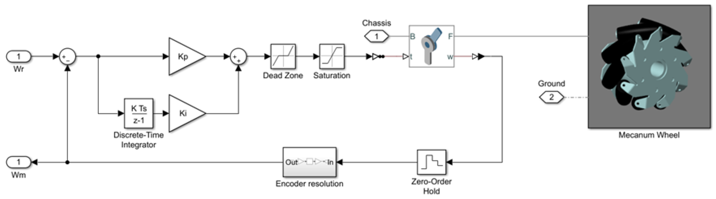
4. Four-Mecanum-Wheeled Mobile Platform

Firstly, the simulation tool developed to test the proposed control solution will be presented in Section 4.1. Secondly, some hardware details about the real platform will be shown in Section 4.2.

4.1. Simulation Tool

Obviously, the best way to test the proposed path-tracking algorithm is by using a real four-mecanum wheeled vehicle. The main issue is that it is not easy to measure the real position of the vehicle. Outdoor positioning (e.g., GPS) does not have enough precision to measure XY coordinates of a small size vehicle. Indoor positioning (e.g., beacons or LIDAR) provides the position with a great amount of noise. To prove the validity of the proposed solutions, a precise way of determining the position and orientation of the vehicle is needed. Simulation tools can be an especially useful alternative, but the simulation model must imitate the behavior of the real model as precisely as possible.

Using transfer functions and kinematic equations of the vehicle excludes some important characteristics of the real vehicle. Nonlinearities of the motors, the limited resolution of the encoders, and the sliding of the wheels play a significant role in the trajectory described by the real vehicle and must be included in the simulation model. Simscape Multibody, a well-known Matlab/Simulink library, is used to develop a simulation model in this work.

In this case, the main challenge is to simulate the real behavior of the mecanum wheel. In a conventional wheel, the friction between the wheel surface and the ground generates the forces and torques that move the vehicle. An example of this for a two-wheeled vehicle can be found in [23]. However, in the case of the mecanum wheel, the forces and torques are generated by the friction with the rollers of the wheel (see Figure 5). The rollers, attached with a 45${}^{\circ }$ angle, allow the wheel to generate a twisting force that makes the vehicle to move in 3 DOF (forward–backwards, right–left, rotation around the vertical axis).

Figure 6 shows the Simscape Multibody model of the mecanum wheel. As can be seen, each one of the rollers has a revolute joint to allow it to turn over the hub in which it is mounted. The contact forces of each one of the rollers can also be seen. These blocks are the ones that generate the combination of forces/torques that make the wheel behave as in the real world.

Each one of the four wheels of the simulated vehicle has its own angular velocity control, as shown in Figure 7. The revolute joint allows the wheel to turn over the vehicle chassis. The damping coefficient in this revolute joint was adjusted to emulate the dynamic behavior of the motor used in the real vehicle. Saturation and dead-zone blocks were included for a better simulation of the real behavior. As the motors used in the real vehicle have good linearity, it was considered necessary to include any other nonlinearities. A PI controller was used to assure that the wheel angular velocity follows its desired reference. This control loop uses the same sample time as the real control loop, implemented in the microcontroller mounted in the vehicle. The parameters on this PI controller are the ones used in the angular velocity control loops of the real vehicle. In the real motor, the angular velocity was measured by means of a built-in encoder. The resolution of this encoder, which depends on the number of pulses-per-revolution, was included in the feedback so that the simulated control loop works with the same information as in the real world.

The simulated control loop was validated by comparison with the real one. With the wheels-in-the-air (i.e, no contact with the ground) and the wheels-on-the-ground, the results provided by the real and simulated encoder are shown in Figure 8a,b. As can be seen, real results have a great amount of noise, but the dynamical behavior is quite similar to the simulated results in the transient and steady state.

Joining four of these structures to the CAD (Computer-Aided Design) model of the chassis, the simulated vehicle is completed, as shown in Figure 9. A Cartesian joint was included to provide XYZ DOF. A Z-axis revolute joint allows the vehicle to turn around its vertical axis. The complete simulation model has four inputs (the angular velocity references) and seven outputs (the angular velocities of the wheels, X and Y position, and orientation of the vehicle). The angular velocities are provided, as measured by the encoders. Position and orientation are provided as if they were measured by a perfect positioning system. To evaluate the proposed algorithms, some noise was added to the outputs to consider the unavoidable uncertainty of the real measurement devices.

To be useful, the simulation model must provide the same information as the real vehicle. Some parameters of the model must be experimentally adjusted, and this can only be achieved by comparing the real response with the simulated one. Some of these parameters are related to the friction of the joints (damping coefficients) that allow the vehicle to move and turn over the floor; however, the most important ones are the parameters involved with the Spatial Contact Forces blocks. Stiffness and damping determine the normal forces that appear when the mecanum wheel rollers touch the ground surface. These forces prevent the vehicle going through the ground, as it happens in the real world. Coefficients of dynamic and static friction determine the frictional forces that make the vehicle move and turn over the ground surface.

Some angular velocity references can be applied to the control loops of the vehicle wheels. The consequent movement of the vehicle (position and orientation) can be measured by processing some images captured by a zenithal camera. The goal is to obtain, with the simulated vehicle, the same outputs when the same inputs are applied.

For the first test, the same reference was applied to the four wheels, which cause a longitudinal (in the direction of the wheels) movement $({(V_x^{ref})}_k^T,{(V_y^{ref})}_k^T=0,{(W_{\psi }^{ref})}_k^T=0)$. Figure 10a shows the results (real and simulated) obtained from this test. As can be seen, the vehicle moves about 1.5 m in the Y direction, and the results are quite similar. The second test applies the same reference to the front-right and back-left wheels and the opposite reference to the other two wheels. These references cause a transversal (perpendicular to the direction of the wheels) movement $({(V_x^{ref})}_k^T=0,{(V_y^{ref})}_k^T,{(W_{\psi }^{ref})}_k^T=0)$. The results are shown in Figure 10b. The vehicle moves about 1.5 m in the X direction, and the simulation model proves to be quite accurate. For the third test, the signs of the references for the right wheels are different from the ones for the left wheels causing a rotational (around the vertical axis) movement $({(V_x^{ref})}_k^T=0,{(V_y^{ref})}_k^T=0,{(W_{\psi }^{ref})}_k^T)$. The results in Figure 10c show that the real vehicle turns approximately at the same velocity as the simulated model.

These comparisons between real and simulated results prove that the simulated vehicle behaves similar to the real one. So, it can be used to test the goodness of the path-tracking algorithms proposed in this work. This will be performed in Section 5.

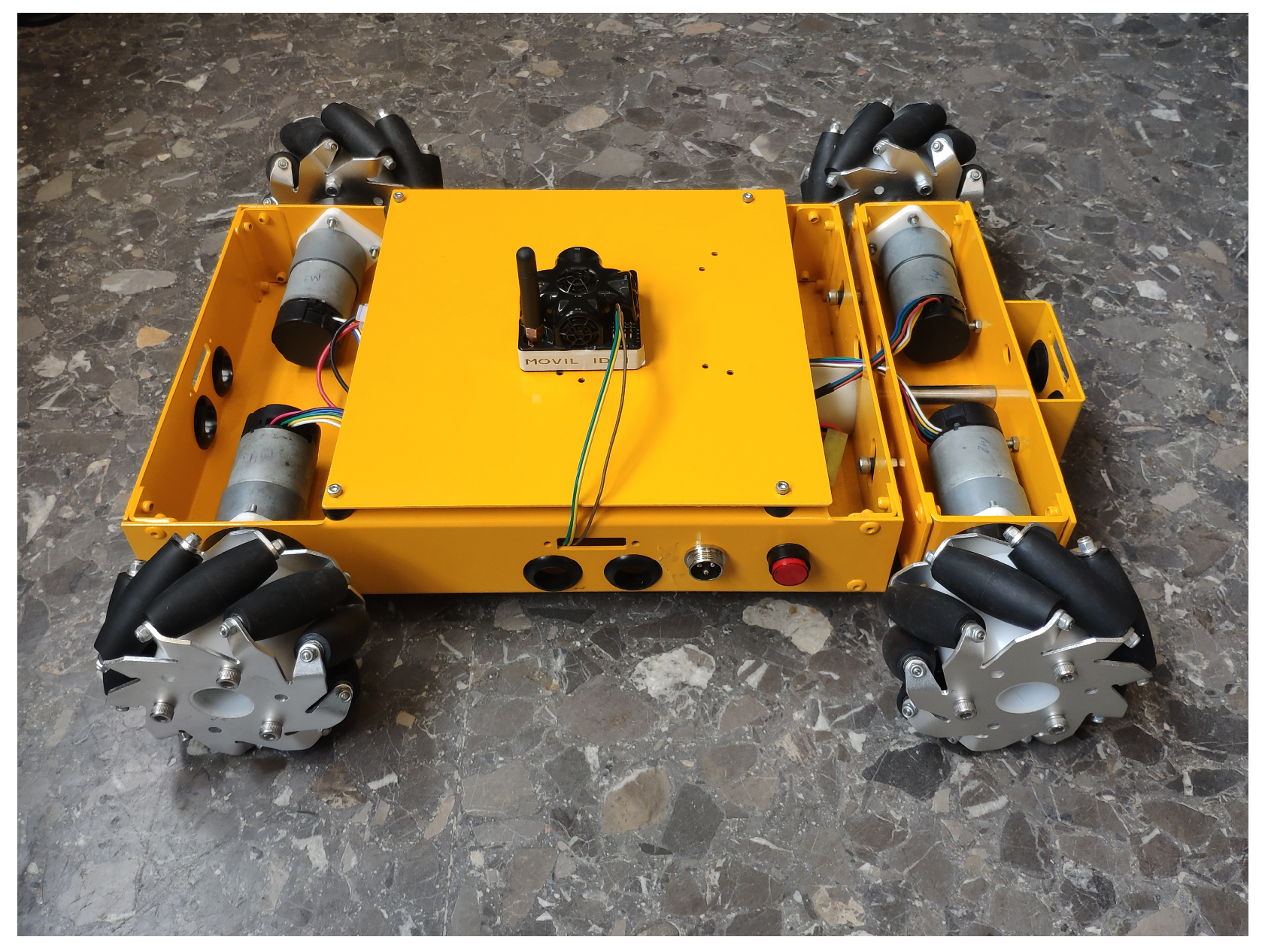
4.2. Real Platform

The reference model for the robot used in the simulator is the NEXUS Robot 4WD Mecanum Wheel Mobile Arduino Robotics Car 10011 (see Figure 11). Some features of the robotic platform are as follows: the body weighs about 3 kg, the wheels weigh 400 g and have 9 rubber rollers, and the parameters related to the kinematic model are (see in Section 3.1) $R=0.05$ m and $L_x=L_y=0.15$ m. More details about the robot can be found in http://www.nexusrobot.com/product/4wd-mecanum-wheel-mobile-arduino-robotics-car-10011.html, accessed on 25 March 2022.

By default, the robotic platform does not include a global positioning system for indoors. For this reason, a beacon-based indoor positioning system—Marvelmind HW v4.9—was integrated (https://marvelmind.com/pics/marvelmind_navigation_system_manual.pdf, accessed on 25 March 2022). The experiments in Section 5.3 were performed in an interference-free environment, where the robot position may be sensed via the Marvelmind beacon system and the robot orientation by means of a Bosch BNO055 Absolute Orientation Sensor (https://www.bosch-sensortec.com/products/smart-sensors/bno055/), accessed on 25 March 2022.

The original metal gearmotor is replaced by a Pololu 37D metal gearmotor (https://www.pololu.com/product/4754, accessed on 25 March 2022) with a gear ratio ($GR$) of 70 and equipped with an integrated quadrature encoder with 64 counts per revolution ($CPR$). In order to transform the $CPR$ into the angular velocity of the wheels ${\omega }_i$, the following equivalence is applied: ${\omega }_i=\frac{2·\pi }{T}·\frac{1}{CPR·GR}·NC$, where $NC$ is the number of counts during the sensing period T. The original hardware was updated by means of a ESP32 with Arduino UNO form factor for compatibility with Adafruit Motor Shield V2 (https://learn.adafruit.com/adafruit-motor-shield-v2-for-arduino), accessed on 25 March 2022. In addition, a DFRobot Gravity—I2C Digital Wattmeter is included (https://www.dfrobot.com/product-1827.html, accessed on 25 March 2022) to measure the voltage and amperage of the battery, and estimate the real voltage injected to the motor by the PWM reference of the Adafruit Motor Shield V2. The code was developed via FREERTOS, a real-time operating system for microcontrollers, which uses a periodic task and the two cores of the ESP32.

5. Simulation Results

This section is organized as follows: The cases simulated are defined in Section 5.1. Some cost indexes are formulated in Section 5.2 with the aim of being used to better assess the results obtained in Section 5.3.

5.1. Cases Evaluated

These are the cases studied in the simulation tool:

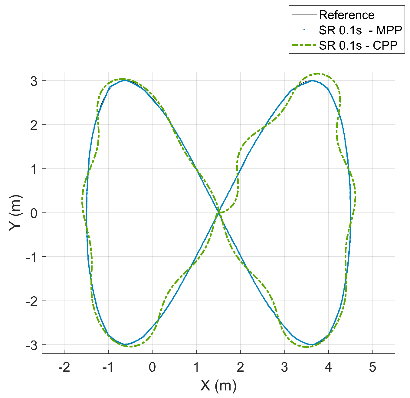
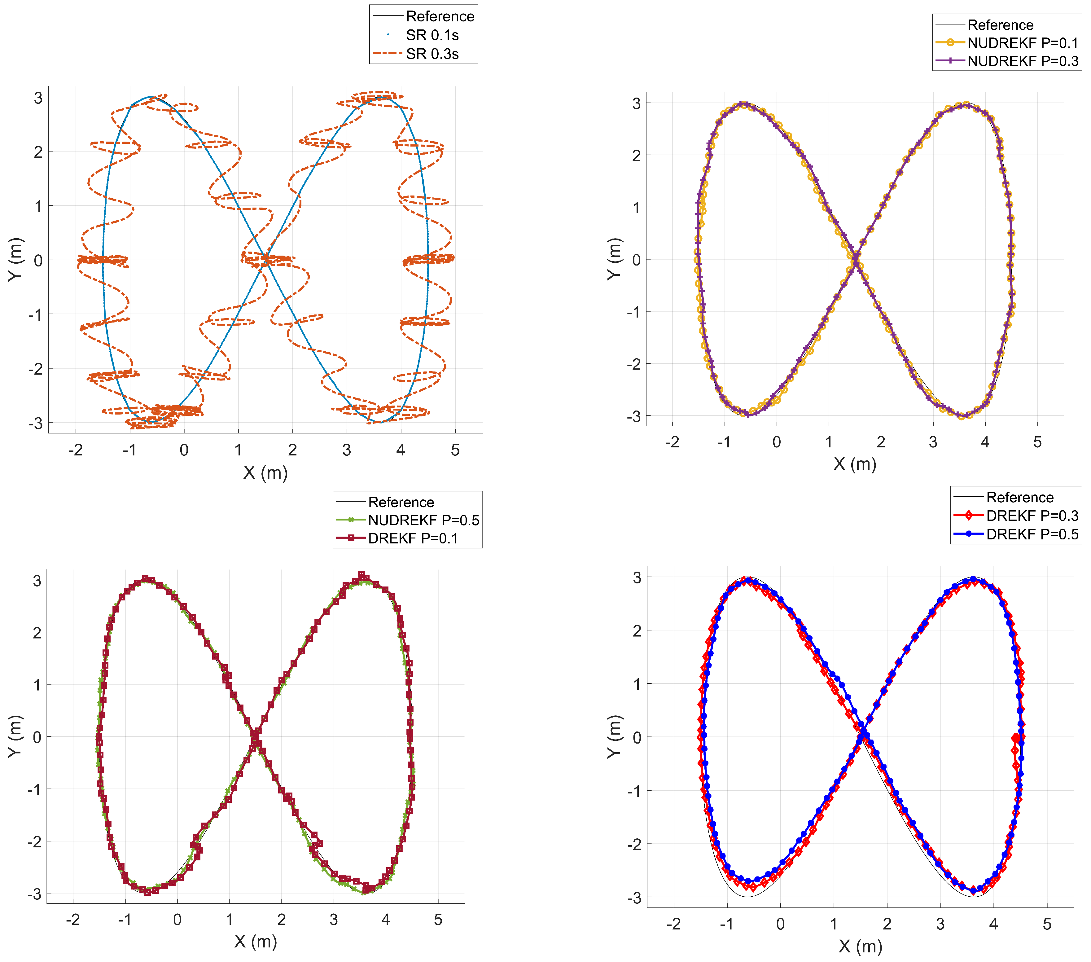
• Direct position, orientation, and angular velocity at single-rate T (SR): In this experiment, output measurements ${({\omega }_1,{\omega }_2,{\omega }_3,{\omega }_4,X,Y,\psi )}_k^T$ are directly sampled from the simulator block at different periods T = 0.1 s and T = 0.3 s. No noise is considered. In addition, for the case SR 0.1 s, the modified version of the Pure Pursuit path-tracking algorithm presented in this work is compared with the original method under the same conditions.
• Dual-rate Extended Kalman Filter (DREKF): This is the filter introduced in [23], which is used in the present work to be compared with the proposed NUDREKF. Gaussian noises are added to the robot outputs: distances ${(d_1,d_2,d_3,d_4)}_k^{NT}$, which are sensed at sampling period $NT$, being N = 10; velocities ${({\omega }_1,{\omega }_2,{\omega }_3,{\omega }_4)}_k^T$; and vehicle orientation ${\left(\psi \right)}_k^T$, which are sampled at period T = 0.1 s. Regarding possible losses of the distance values, three options for the loss probability P are simulated: $\mathit{P}=0.1$, $\mathit{P}=0.3$, and $\mathit{P}=0.5$. Due to the nature of the DREKF, if one or more distances are lost at the current sensing time, the full set of distances will be considered lost.
• Nonuniform dual-rate extended Kalman filter (NUDREKF): This is the case presented in Section 3.2. The simulations are carried out under the same considerations as in the DREKF scenario; now, however, as the NUDREKF is able to face nonuniform sampling patterns, individual losses for each distance can be treated.

The reference trajectory to be tracked is the Lissajous curve $(1,2)$ shown in Figure 12, where the subset of via-points can also be seen.

5.2. Cost Indexes for Performance Assessment

To better quantify the results to be shown in Section 5.3, four cost indexes will be used. These indexes evaluate control performance for every case simulated with the aim of making the comparison easier. The cost indexes are as follows:

• $J_1$, which is based on the ${\ell }_2$-norm, and its goal is to provide a measure (in meters) about how accurately the path is followed:

  $$J_1=\frac{1}{l}\sum _{k=1}^l\underset{1\le k^{\prime }\le l}{min}\sqrt{{\left(X_k^T-{\left(X^{ref}\right)}_{k^{\prime }}^T\right)}^2+{\left(Y_k^T-{\left(Y^{ref}\right)}_{k^{\prime }}^T\right)}^2}$$

  (19)

  where l is the number of iterations at period T required by the vehicle to reach the final point of the path, ${(X,Y)}_k^T$ is the current vehicle position, and ${(X^{ref},Y^{ref})}_{k^{\prime }}^T$ is the nearest kinematic position reference to the current vehicle position. It is worth noting that, despite using a dual-rate control scheme, the position data may be available at period T (intersample behavior; see, e.g., [40]) in the simulator environment.
• $J_2$, which is based on the ${\ell }_{\infty }$-norm and is defined to know the maximum difference (in meters) between the desired path and the current vehicle position:

  $$J_2=\underset{1\le k\le l}{max}\left\{\underset{1\le k^{\prime }\le l}{min}\sqrt{{\left(X_k^T-{\left(X^{ref}\right)}_{k^{\prime }}^T\right)}^2+{\left(Y_k^T-{\left(Y^{ref}\right)}_{k^{\prime }}^T\right)}^2}\right\}$$

  (20)
• $J_3$, which measures the total amount of time (in seconds) elapsed to arrive at the final destination:

  $$J_3=lT$$

  (21)
• $J_4$, which is based on the ${\ell }_2$-norm, and its goal is to provide a measure (in meters) about how accurately the estimation is made:

  $$J_4=\frac{1}{l}\sum _{k=1}^l\sqrt{{\left(X_k^T-{\widehat{X}}_k^T\right)}^2+{\left(Y_k^T-{\widehat{Y}}_k^T\right)}^2}$$

  (22)

  where ${(\widehat{X},\widehat{Y})}_k^T$ is the estimated vehicle position.

5.3. Results

First of all, let us compare the modified Pure Pursuit path-tracking algorithm with the original, conventional version under the same conditions and for SR 0.1 s.

Figure 13 clearly reveals the benefits of using the modified proposal (MPP) versus the original, conventional one (CPP)—that is, MPP is able to track the path more accurately than CPP. This fact is confirmed by the cost indexes presented in

Table 1. Cost index results for Pure Pursuit comparison.

	${\mathit{J}}_1$	${\mathit{J}}_2$	${\mathit{J}}_3$
SR 0.1 s—Modified Pure Pursuit (MPP)	1.0	1.0	1.0
SR 0.1 s—Conventional Pure Pursuit (CPP)	14.3	6.96	0.79

, where $J_1$ and $J_2$ are noticeably worsened for the original algorithm. However, $J_3$ points out a slight reduction of time that CPP needs to take in order to follow the trajectory. Note that the indexes are divided by the best case—that is, the SR 0.1 s MPP.

Then, adopting the modified Pure Pursuit algorithm for the rest of simulations, Figure 14, Figure 15 and Figure 16 show the results obtained for the Lissajous curve.

Table 2. Cost index results.

	${\mathit{J}}_1$	${\mathit{J}}_2$	${\mathit{J}}_3$	${\mathit{J}}_4$
SR 0.1 s	1.0	1.0	1.0	-
SR 0.3 s	42.8	17.5	2.7	-
NUDREKF $\mathit{P}$ = 0.1	4.8	2.4	1.1	1.0
NUDREKF $\mathit{P}$ = 0.3	5.3	3.4	1.1	1.1
NUDREKF $\mathit{P}$ = 0.5	5.5	3.6	1.1	1.3
DREKF $\mathit{P}$ = 0.1	6.9	5.2	1.2	1.5
DREKF $\mathit{P}$ = 0.3	9.4	6.4	1.0	1.9
DREKF $\mathit{P}$ = 0.5	12.2	9.3	1.0	2.6

presents the cost indexes calculated for every case, where the cost indexes $J_1,J_2$, and $J_3$ are divided by the nominal case—that is, the single-rate case at T = 0.1 s (SR 0.1 s)—and $J_4$ is divided by the best case—that is, NUDREKF $\mathit{P}$ = 0.1.

The main conclusions of the comparison are as follows:

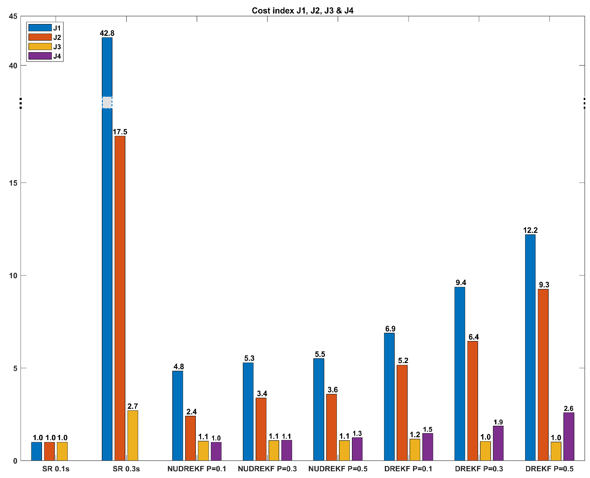
• Cost index $J_3$ presents values very similar to the nominal one for every case, except for SR 0.3 s—that is, the case where direct measurements are sensed at sampling period T = 0.3 s, which has a value 2.7 times higher.
• SR 0.3 s shows the worst behavior (noticeable oscillations), which is confirmed by the clear rise of every cost index. On average, $J_1$ and $J_2$ increase their values by $42.8$ and $17.5$ times, respectively.
• In general, the NUDREKF cost indices are lower than the DREKF cost indices when appearing in nonuniform sampling patterns, beyond managing noisy and scarce data, and existing process nonlinearities. As can be seen in Figure 14, the higher P is, the worse the cost value will be. This rule is more evident for the DREKF. Note that the worst case for NUDREKF—that is, when $\mathit{P}$ = 0.5—presents lower $J_1$, $J_2$, and $J_4$ than the best case for DREKF—that is, when $\mathit{P}$ = 0.1.
• NUDREKF $\mathit{P}$ = 0.1 shows accurate path tracking, despite having scarce position measurements (10 less times), and assuming dropouts, noise, and nonlinearities. The cost indexes confirm the achievement of satisfactory control properties, since $J_1$ and $J_2$ are slightly worsened with respect to the nominal case (4.8 and 2.4 times higher, respectively). NUDREKF $\mathit{P}$ = 0.3 shows slightly worse path tracking with respect to NUDREKF $\mathit{P}$ = 0.1, increasing 0.5, 1, and 0.3 points in $J_1$, $J_2$, and $J_4$, respectively. NUDREKF $\mathit{P}$ = 0.5 worsens the path-tracking behavior a bit more regarding NUDREKF $\mathit{P}$ = 0.1, and increases 0.7, 1.2, and 0.5 points in $J_1$, $J_2$, and $J_4$, respectively. In summary, the NUDREKF strategy preserves a satisfactory trajectory tracking performance under conditions of loss of measurements.
• In contrast, DREKF $\mathit{P}$ = 0.1 shows slightly worse path tracking with respect to NUDREKF $\mathit{P}$ = 0.5, and quite worse behavior regarding NUDREKF $\mathit{P}$ = 0.1. As can be seen in Figure 15, DREKF $\mathit{P}$ = 0.3 and DREKF $\mathit{P}$ = 0.5 seem to achieve good path tracking; however, the correction of the position is taken only a few times and it is generally based on odometry measurements, obtaining poor performance on the cost index $J_1$, $J_2$ and $J_4$. If the experiment were extended over time, the tracking would suffer from drift in the estimation of the robot.
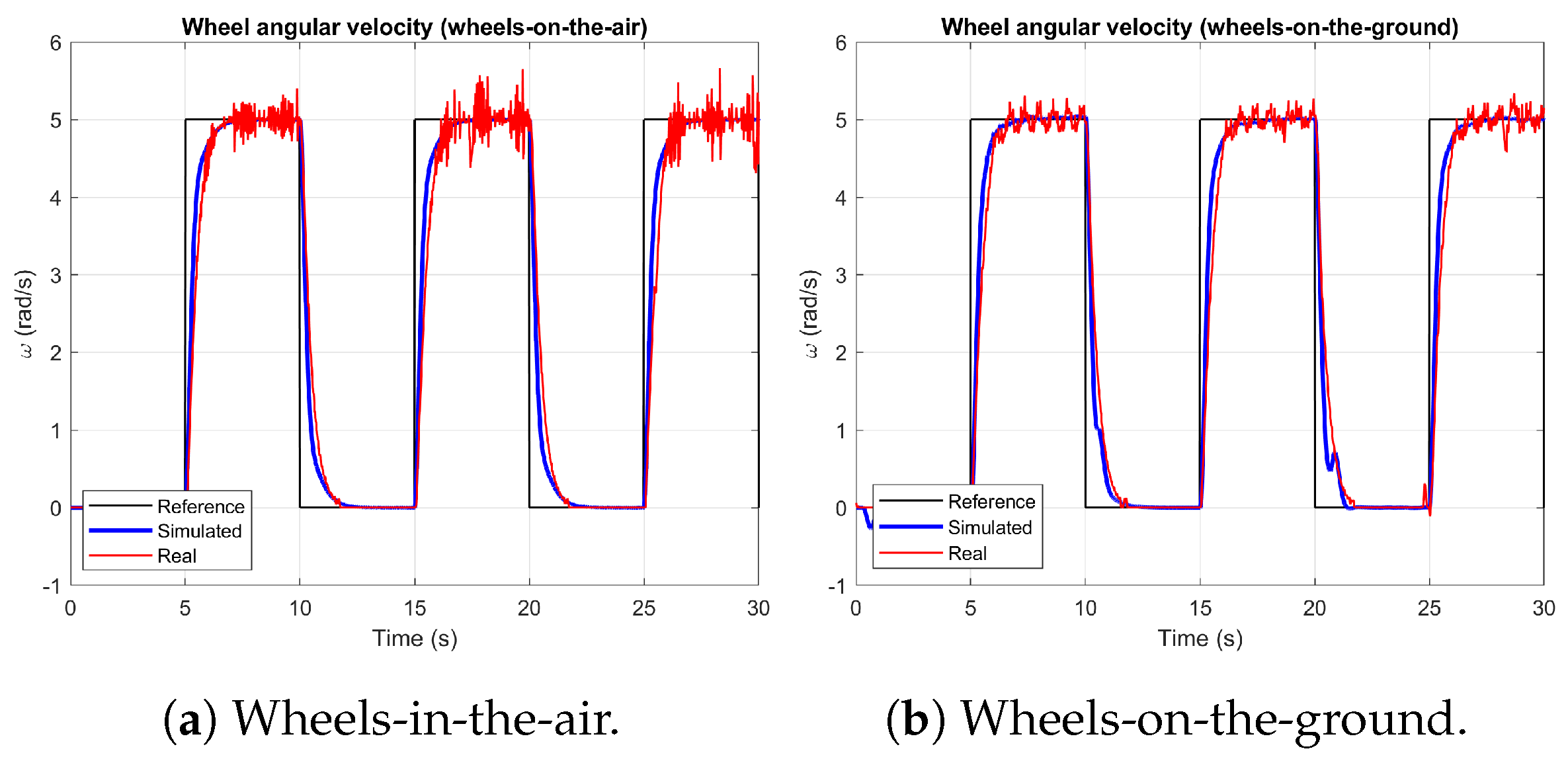
• Figure 16 depicts the path-tracking trajectory error for the different cases evaluated. As expected (see Figure 16a), SR 0.1 s presents the lowest error, being practically null except for the four slight spikes corresponding to the four curves of the trajectory, and SR 0.3 s shows the highest error, which reaches up to 0.6 m. Between both single-rate cases, the error value for the dual-rate approaches can be found. As can be seen in Figure 16b,c, NUDREKF cases depict lower error (up to 0.1 m) than DREKF cases (which can reach up to 0.3 m). This fact confirms the previous conclusions about the improvement introduced by the nonuniform sampling strategy.

As a summary, the proposed NUDREKF strategy enables us to reach a satisfactory path-tracking performance, despite considering possible nonuniform patterns of loss of data. To check the possibilities and power of the simulation tool developed, the next link to one video that shows the cases evaluated is provided: https://1drv.ms/v/s!AgyvxPGH2rA4ezbNYsz7S1O6xqg, accessed on 25 March 2022.

6. Conclusions

The proposed nonuniform dual-rate extended Kalman filter solves the problem of estimating the state of a vehicle from output measurements sensed at different periods and with possible nonuniform loss of data, despite existing nonlinearities and noises. The modified Pure Pursuit path-tracking algorithm is a useful procedure for precise reference tracking of the four-mecanum-wheeled mobile platform along a curved path. The simulation application based on Simscape Multibody is a powerful tool to test the control structure proposed.

References

- Safar, M.J.A. Holonomic and omnidirectional locomotion systems for wheeled mobile robots: A review. J. Teknol. 2015, 77, 91–97. [Google Scholar]
- Wang, C.; Liu, X.; Yang, X.; Hu, F.; Jiang, A.; Yang, C. Trajectory tracking of an omni-directional wheeled mobile robot using a model predictive control strategy. Appl. Sci. 2018, 8, 231. [Google Scholar] [CrossRef] [Green Version]
- Wada, M.; Mori, S. Holonomic and omnidirectional vehicle with conventional tires. In Proceedings of the IEEE International Conference on Robotics and Automation, Minneapolis, MI, USA, 22–28 April 1996; Volume 4, pp. 3671–3676. [Google Scholar]
- Doroftei, I.; Grosu, V.; Spinu, V. Omnidirectional Mobile Robot-Design and Implementation; INTECH Open Access Publisher: London, UK, 2007. [Google Scholar]
- Ilon, B.E. Wheels for a Course Stable Selfpropelling Vehicle Movable in Any Desired Direction on the Ground or Some Other Base. U.S. Patent 3,876,255, 8 April 1975. [Google Scholar]
- Adăscăliţei, F.; Doroftei, I. Practical applications for mobile robots based on mecanum wheels-a systematic survey. Rom. Rev. Precis. Mech. Opt. Mechatron. 2011, 40, 21–29. [Google Scholar]
- Xie, L.; Scheifele, C.; Xu, W.; Stol, K.A. Heavy-duty omni-directional Mecanum-wheeled robot for autonomous navigation: System development and simulation realization. In Proceedings of the 2015 IEEE International Conference on Mechatronics (ICM), Nagoya, Japan, 6–8 March 2015; pp. 256–261. [Google Scholar]
- Aguiar, A.P.; Hespanha, J.P. Trajectory-tracking and path-following of underactuated autonomous vehicles with parametric modeling uncertainty. IEEE Trans. Autom. Control 2007, 52, 1362–1379. [Google Scholar] [CrossRef] [Green Version]
- Coulter, R.C. Implementation of the Pure Pursuit Path Tracking Algorithm; Technical Report; Carnegie-Mellon UNIV Pittsburgh PA Robotics INST: Pittsburgh, PA, USA, 1992. [Google Scholar]
- Fue, K.; Porter, W.; Barnes, E.; Li, C.; Rains, G. Autonomous Navigation of a Center-Articulated and Hydrostatic Transmission Rover using a Modified Pure Pursuit Algorithm in a Cotton Field. Sensors 2020, 20, 4412. [Google Scholar] [CrossRef] [PubMed]
- Mitchell, S.; Sajjad, I.; Al-Hashimi, A.; Dadras, S.; Gerdes, R.M.; Sharma, R. Visual distance estimation for pure pursuit based platooning with a monocular camera. In Proceedings of the 2017 American Control Conference (ACC), Seattle, WA, USA, 24–26 May 2017; pp. 2327–2332. [Google Scholar]
- Chopp, D.J.; Spike, N.; Bos, J.; Robinette, D. Multi point pure pursuit. In Proceedings of the Autonomous Systems: Sensors, Processing, and Security for Vehicles and Infrastructure 2020, International Society for Optics and Photonics, Online, 27 April–8 May 2020; Volume 11415, p. 1141505. [Google Scholar]
- Gámez Serna, C.; Lombard, A.; Ruichek, Y.; Abbas-Turki, A. GPS-based curve estimation for an adaptive pure pursuit algorithm. In Proceedings of the Mexican International Conference on Artificial Intelligence, Cancun, Mexico, 23–28 October 2016; pp. 497–511. [Google Scholar]
- Wang, H.; Chen, X.; Chen, Y.; Li, B.; Miao, Z. Trajectory tracking and speed control of cleaning vehicle based on improved pure pursuit algorithm. In Proceedings of the 2019 Chinese Control Conference (CCC), Guangzhou, China, 27–30 July 2019; pp. 4348–4353. [Google Scholar]
- Ohta, H.; Akai, N.; Takeuchi, E.; Kato, S.; Edahiro, M. Pure pursuit revisited: Field testing of autonomous vehicles in urban areas. In Proceedings of the 2016 IEEE 4th International Conference on Cyber-Physical Systems, Networks, and Applications (CPSNA), Nagoya, Japan, 6–7 October 2016; pp. 7–12. [Google Scholar]
- Haykin, S. Kalman Filtering and Neural Networks; Wiley Online Library: Hoboken, NJ, USA, 2001. [Google Scholar]
- Welch, G.; Bishop, G. An Introduction to the Kalman Filter; University of North Carolina: Chapel Hill, NC, USA, 2006; Volume 378. [Google Scholar]
- Simon, D. Optimal State Estimation: Kalman, H Infinity, and Nonlinear Approaches; John Wiley & Sons: Hoboken, NJ, USA, 2006. [Google Scholar]
- Garcia, R.; Pardal, P.; Kuga, H.; Zanardi, M. Nonlinear filtering for sequential spacecraft attitude estimation with real data: Cubature Kalman Filter, Unscented Kalman Filter and Extended Kalman Filter. Adv. Space Res. 2019, 63, 1038–1050. [Google Scholar] [CrossRef]
- Grillo, C.; Vitrano, F. State estimation of a nonlinear unmanned aerial vehicle model using an Extended Kalman Filter. In Proceedings of the 15th AIAA International Space Planes and Hypersonic Systems and Technologies Conference, Dayton, OH, USA, 28 April–1 May 2008; p. 2529. [Google Scholar]
- Mora, M.C.; Piza, R.; Tornero, J. Multirate obstacle tracking and path planning for intelligent vehicles. In Proceedings of the 2007 IEEE Intelligent Vehicles Symposium, Istanbul, Turkey, 13–15 June 2007; pp. 172–177. [Google Scholar]
- Salt Ducajú, J.M.; Salt Llobregat, J.J.; Cuenca, Á.; Tomizuka, M. Autonomous Ground Vehicle Lane-Keeping LPV Model-Based Control: Dual-Rate State Estimation and Comparison of Different Real-Time Control Strategies. Sensors 2021, 21, 1531. [Google Scholar] [CrossRef] [PubMed]
- Carbonell, R.; Cuenca, Á.; Casanova, V.; Pizá, R.; Salt Llobregat, J.J. Dual-Rate Extended Kalman Filter Based Path-Following Motion Control for an Unmanned Ground Vehicle: Realistic Simulation. Sensors 2021, 21, 7557. [Google Scholar] [CrossRef]
- Gopalakrishnan, A.; Kaisare, N.S.; Narasimhan, S. Incorporating delayed and infrequent measurements in Extended Kalman Filter based nonlinear state estimation. J. Process Control 2011, 21, 119–129. [Google Scholar] [CrossRef]
- Wang, J.; Alipouri, Y.; Huang, B. Multirate Sensor Fusion in the Presence of Irregular Measurements and Time-Varying Time Delays Using Synchronized, Neural, Extended Kalman Filters. IEEE Trans. Instrum. Meas. 2021, 71, 1–9. [Google Scholar] [CrossRef]
- Szántó, A.; Hajdu, S. Vehicle Modelling and Simulation in Simulink. Int. J. Eng. Manag. Sci. 2019, 4, 260–265. [Google Scholar] [CrossRef]
- Crenganiş, M.; Breaz, R.E.; Racz, S.G.; Biriş, C.M.; Gîrjob, C.E.; Maroşan, A.I. Development of a lightweight multipurpose high mobility vehicle for use in confined spaces. In Proceedings of the 2021 International Automatic Control Conference (CACS), Qingdao, China, 17–21 July 2021; pp. 1–6. [Google Scholar]
- Arora, R.; Singh, R. Physical Modeling of the Tread Robot and Simulated on Even and Uneven Surface. In Proceedings of the International Conference on Intelligent Systems Design and Applications, Vellore, India, 6–8 December 2018; pp. 173–181. [Google Scholar]
- Vitolo, F.; Rega, A.; Di Marino, C.; Pasquariello, A.; Zanella, A.; Patalano, S. Mobile Robots and Cobots Integration: A Preliminary Design of a Mechatronic Interface by Using MBSE Approach. Appl. Sci. 2022, 12, 419. [Google Scholar] [CrossRef]
- Dosoftei, C.; Horga, V.; Doroftei, I.; Popovici, T.; Custura, Ş. Simplified Mecanum Wheel Modelling using a Reduced Omni Wheel Model for Dynamic Simulation of an Omnidirectional Mobile Robot. In Proceedings of the International Conference and Exposition on Electrical and Power Engineering (EPE), Iasi, Romania, 22–23 October 2020; pp. 721–726. [Google Scholar]
- Bayar, G.; Ozturk, S. Investigation of the effects of contact forces acting on rollers of a mecanum wheeled robot. Mechatronics 2020, 72, 102467. [Google Scholar] [CrossRef]
- Siegwart, R.; Nourbakhsh, I.; Scaramuzza, D. Introduction to Autonomous Mobile Robots, 2nd ed.; MIT Press: Cambridge, MA, USA, 2011. [Google Scholar]
- Diegel, O.; Badve, A.; Bright, G.; Potgieter, J.; Tlale, S. Improved mecanum wheel design for omni-directional robots. In Proceedings of the 2002 Australasian Conference on Robotics and Automation, Auckland, New Zealand, 27–29 November 2002; pp. 117–121. [Google Scholar]
- Tornero, J.; Tomizuka, M.; Camina, C.; Ballester, E.; Piza, R. Design of dual-rate PID controllers. In Proceedings of the 2001 IEEE International Conference on Control Applications (CCA’01) (Cat. No.01CH37204), Mexico City, Mexico, 7 September 2001; pp. 859–865. [Google Scholar] [CrossRef]
- Tornero, J.; Piza, R.; Albertos, P.; Salt, J. Multirate LQG controller applied to self-location and path-tracking in mobile robots. In Proceedings of the 2001 IEEE/RSJ International Conference on Intelligent Robots and Systems, Expanding the Societal Role of Robotics in the the Next Millennium (Cat. No. 01CH37180), Maui, HI, USA, 29 October–3 November 2001; Volume 2, pp. 625–630. [Google Scholar] [CrossRef]
- Pizá, R.; Tornero, J.; Tomizuka, M. Self-localization and path-tracking in mobile robots. Dual-rate Kalman filtering. In Proceedings of the International Conference on Systems Identification and Control Problems, Moscow, Russia, 26–28 September 2000. [Google Scholar]
- Tornero, J. Non-Conventional Sampled Data Systems Modelling; Control System Centre Report nº 640/1985; University of Manchester (UMIST): Manchester, UK, 1985. [Google Scholar]
- Longhi, S. Structural properties of multirate sampled-data systems. IEEE Trans. Autom. Control 1994, 39, 692–696. [Google Scholar] [CrossRef]
- Kawabata, K.; Ma, L.; Xue, J.; Zhu, C.; Zheng, N. A path generation for automated vehicle based on Bezier curve and via-points. Robot. Auton. Syst. 2015, 74, 243–252. [Google Scholar] [CrossRef]
- Salt, J.; Albertos, P. Model-based multirate controllers design. IEEE Trans. Control. Syst. Technol. 2005, 13, 988–997. [Google Scholar] [CrossRef]