Article

Relationship between Subjective and Biological Responses to Comfortable and Uncomfortable Sounds

Department of Mechanical Engineering, Faculty of Science and Technology, Tokyo University of Science, Tokyo 162-8601, Japan
Appl. Sci. 2022, 12(7), 3417; https://doi.org/10.3390/app12073417
Submission received: 5 February 2022 / Revised: 23 March 2022 / Accepted: 25 March 2022 / Published: 27 March 2022

Abstract

:
Various kinds of biological sensors are now embedded in wearable devices and data on human biological information have recently become more widespread. Among various environmental stressors, sound has emotional and biological impacts on humans, and it is worthwhile to investigate the relationship between the subjective impressions of and biological responses to such sounds. In this study, the relationship between subjective and biological responses to acoustic stimuli with two contrasting kinds of sounds, a murmuring river sound and white noise, was investigated. The subjective and biological responses were measured during the presentation of the sounds. Compared with the murmuring river sound, the white noise had a significantly decreased EEG-related index of α-EEG and HRV-related index of SD2/SD1. The correlation between each index of subjective and biological responses indicated that α-EEG was highly correlated with the results of subjective evaluation. However, based on a more detailed analysis with clustering, some subjects showed different biological responses in each trial since they felt the sound was powerful when listening to the murmuring river sound, as well as feeling that it was beautiful. It was suggested that biological responses to sound exposure may be affected by the impression of the sound, which varies by individual.

1. Introduction

In 2014, a basic survey on industrial safety and health conducted by the Japanese Ministry of Health, Labour and Welfare (MHLW) showed that more than 1.11 million patients suffer from mood disorders such as depression, and that the number has been rising annually. In contrast, on a global level, over 300 million people are estimated to suffer from depression, equivalent to 4.4% of the world’s population [1]. One of the major reasons for this situation is the stress caused by various kinds of tension and anxiety in modern life. To make our lives more comfortable, living environments should be designed to be suitable from both physiological and psychological perspectives.
Firstly, physiological function is mainly regulated by central nervous system activity and peripheral nervous system activity. While the function of central nervous system responses can be evaluated through background and evoked electroencephalographs (EEGs), which record the electrical activity of the brain, the function of peripheral nervous system responses can be evaluated through cardiovascular activities such as by electrocardiogram [2,3], reflecting the heart rate, blood pressure [4] and vasomotor activity [5], which indicate autonomic nervous system activity, and other factors such as respiration [6], skin temperature [7], and eye movements [8]. In recent years, many studies on brain science have been conducted, and objective interpretations of how the brain is related to psychological functions have also been studied [9]. A brain wave is an electrical pattern of brain activity. EEGs are typically described in terms of rhythmic activity and transient activity. The former type of brain wave activity constitutes alpha waves, beta waves, gamma waves, and lambda waves. Other than these frequency components, delta and theta waves in the lower frequencies under 8 Hz have also been treated. Alpha waves are found in the frequency range from 8 Hz to 13 Hz [10]. Hans Berger firstly named this rhythmic EEG activity as an “alpha wave” [11]. These rhythmic waves differ in frequency. For example, the rhythmic wave in the alpha domain can be observed when closing the eyes and with relaxation. The mechanism of exciting these various frequency components has been investigated; however, physiological changes including brain activities in response to emotional stimuli are not simple linear responses, but rather are assumed to be complex [3,12]. The measurement of psychological functions is generally based on a subjective evaluation. However, since the results of subjective evaluations vary widely among individuals, it may be beneficial to combine them with an objective evaluation method using physiological indicators in order to bring universality to evaluations. To use such a combined method with subjective and objective evaluations, it is first necessary to clarify the relationship between physiological and psychological functions.
We are constantly exposed to various kinds of environmental stimuli in our daily lives. For example, from an acoustic viewpoint, environmental noise, such as that from a train station or a construction site, can be perceived as “unpleasant” if it is too loud, and may thus cause stress. On the other hand, listening to a murmuring river, birdsong, or classical music can be perceived as “pleasant”. It is thought that the latter type of stimuli may have a stress-reducing effect. For example, the effects of water sounds on reducing stress have been investigated; however, these depend on the individual situation [13]. Even when listening to pleasant sounds, some people may feel uncomfortable due to other factors. However, if the subjective and objective evaluations have a relatively strong relationship, the effects of the surrounding environment on humans can be accurately assessed using a combination of methods.
Regarding the mechanism of emotional and biological responses to sounds, it has been reported that music perception involves complex brain functions, potentially affecting emotion and influencing the autonomic nervous system [14]. In a study of the EEG responses of subjects listening to their preferred and non-preferred music, the power of alpha waves increased when listening to their preferred music [15]. Many studies on the relationship between auditory stimuli and EEG, such as a study that measured EEG when Mozart’s music was presented [16], can be seen. In the other study, the effect of music preference on brain waves was studied using classical and rock music [17]. As described above, the auditory effect of comfortable music on brain waves has been investigated, but the auditory stimuli of music consist of many sounds and complex structures, and their effect on humans is also considered to be complex. In contrast, natural sounds such as river sounds are simple, and they may provide relaxation to humans [18]. However, the auditory effect of such a comfortable sound on a human’s brain wave has barely been discussed in detail.
On the other hand, heart rate variability (HRV) has also been utilized as an indicator of many physiological and behavioral factors [19] such as stress [20], fatigue [21], and performance [22]. The relationship between HRV and other biological conditions such as autonomic nervous function has been investigated [23]. While the relationship among various biological indicators has been generally discussed, HRV and EEG are often investigated together [24] since both provide cyclic time-transient data and are relatively easy to measure. The synchronicity of HRV and EEG is often analyzed and applied to various cases [25]; however, the relationship between HRV and EEG in response to sound stimulation has rarely been studied. As mentioned above, it is clear that sound has an emotional and biological impact on humans, and it is worthwhile to investigate such a mechanism; it will be beneficial to investigate the relationship between the subjective impressions and biological responses caused by sounds using HRV and EEG.
The purpose of this study is to evaluate the effects of auditory stimuli comparing two kinds of sounds, white noise and a murmuring river sound, using psychological and physiological responses. Through such a study, a basic understanding of how auditory stimuli affect both psychological and physiological states of humans can be confirmed. So, in this study, using EEG and HRV as the means of physiological evaluation, the relationship between subjective impressions and biological responses is discussed.
Firstly, the experimental methods of subjective and biological measurements are described in Section 2. The subjective impressions of the white noise and murmuring river sound were measured by a subjective evaluation test using the semantic differential (SD) method. After this, the biological parameters related to EEG and HRV were physiologically measured for each of the subjects. In Section 3, the subjective and physiological results are comparatively discussed. Then, we determine whether some of the biological parameters of EEG and HRV are significantly related to the comfortableness of the reproduced sound. However, some subjects decreased their alpha wave energy of the EEG and indicated different responses to the comfortable sound of murmuring river compared to the majority of the subjects who showed an increase in alpha wave energy. A minority of subjects had slightly different auditory impressions of the murmuring river sound where they felt some negativity toward it. Finally, it has been indicated that individuals have different impressions of sound, but the relationship between subjective impressions and biological responses shows a consistent trend.

2. Methods

Psychological and physiological evaluation experiments to examine the effects of auditory stimuli on subjective and biological responses were conducted. Firstly, the subjective impressions caused by two kinds of sounds were determined based on the results of the subjective evaluation experiment, and the obtained results were compared to the biological responses relevant to EEGs and HRV.

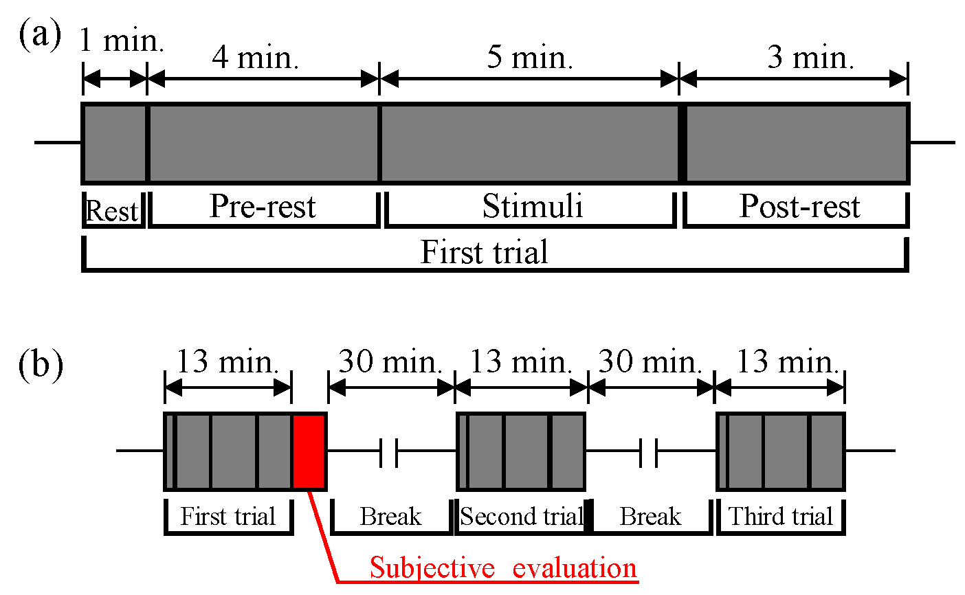
2.1. Outline of the Experiment

Eight healthy males with normal hearing in their twenties were selected as the subjects of the experiment. It should be noted that in this research the relationship between the subjective and biological response on sound representation was assessed. So, the subjects were university students in their twenties. However, it should also be noted that, ideally, subjects should be selected from a large population of various ages, if one wants to determine the effect of the subjects’ age on their interpretations. The method of the experiment is shown in Figure 1. After a one-minute period in which the subjects familiarized themselves with the experimental environment, they had a four-minute pre-resting period, listened to a five-minute-long auditory stimulus, and then had a three-minute post-resting period, for a total of 12 min. After completing the experiment, a subjective evaluation of the subjects’ impressions of the presented sounds was conducted. To verify the reproducibility of this experiment, the experiments were repeated three times under the same experimental conditions as shown in Figure 1b. To prevent the disturbance of brain waves and heart rates caused by visual stimuli as much as possible, the experiment was conducted in a dark room, shown in Figure 2a. In addition, to avoid artifacts such as muscle potential and eye movement, each subject was instructed to relax in a seated position with their eyes closed during the experiment. To prevent fatigue, all three experiments were conducted with a 30 min break between each trial.
Two types of stationary auditory stimuli were used: white noise and the murmuring sound of a river. Hereafter, the white noise condition is indicated as “SA”, while the murmuring river condition is indicated as “SB”. The sounds were listened to using in-ear headphones (Etymotic Research, ER-4s). The reason for using in-ear headphones was that they were not expected to interfere with the wearing of an EEG headset. In addition, ER-4s were chosen since they have a frequency response that is as flat as possible. The A-weighted equivalent sound pressure levels (LAeq) of the reproduced sounds were set to 60 dB for both sounds.

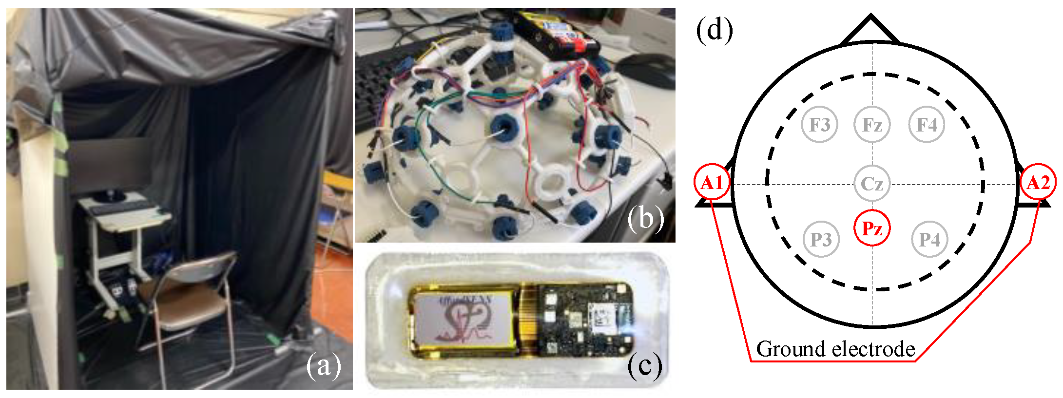
2.2. Physiological Measurement
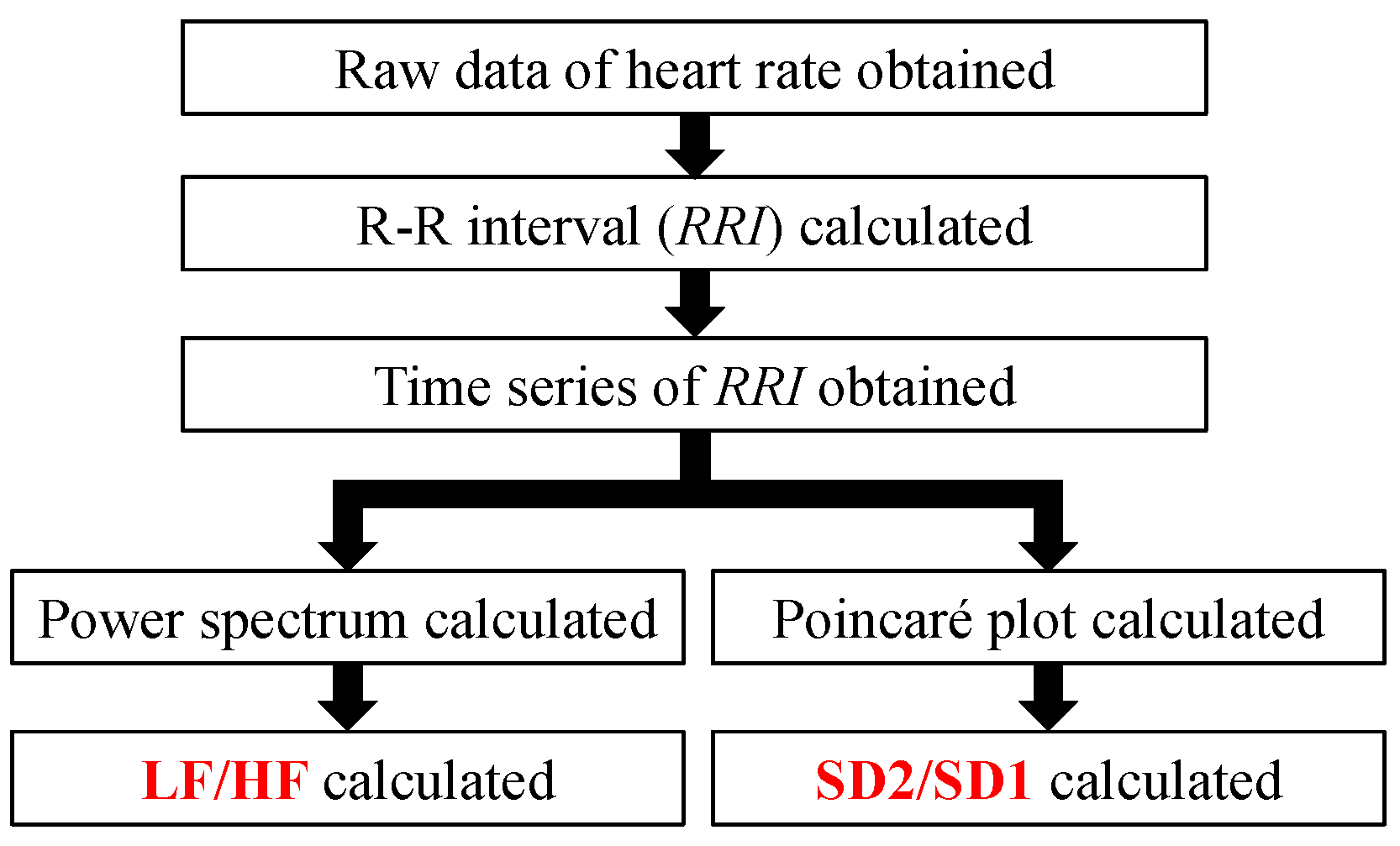
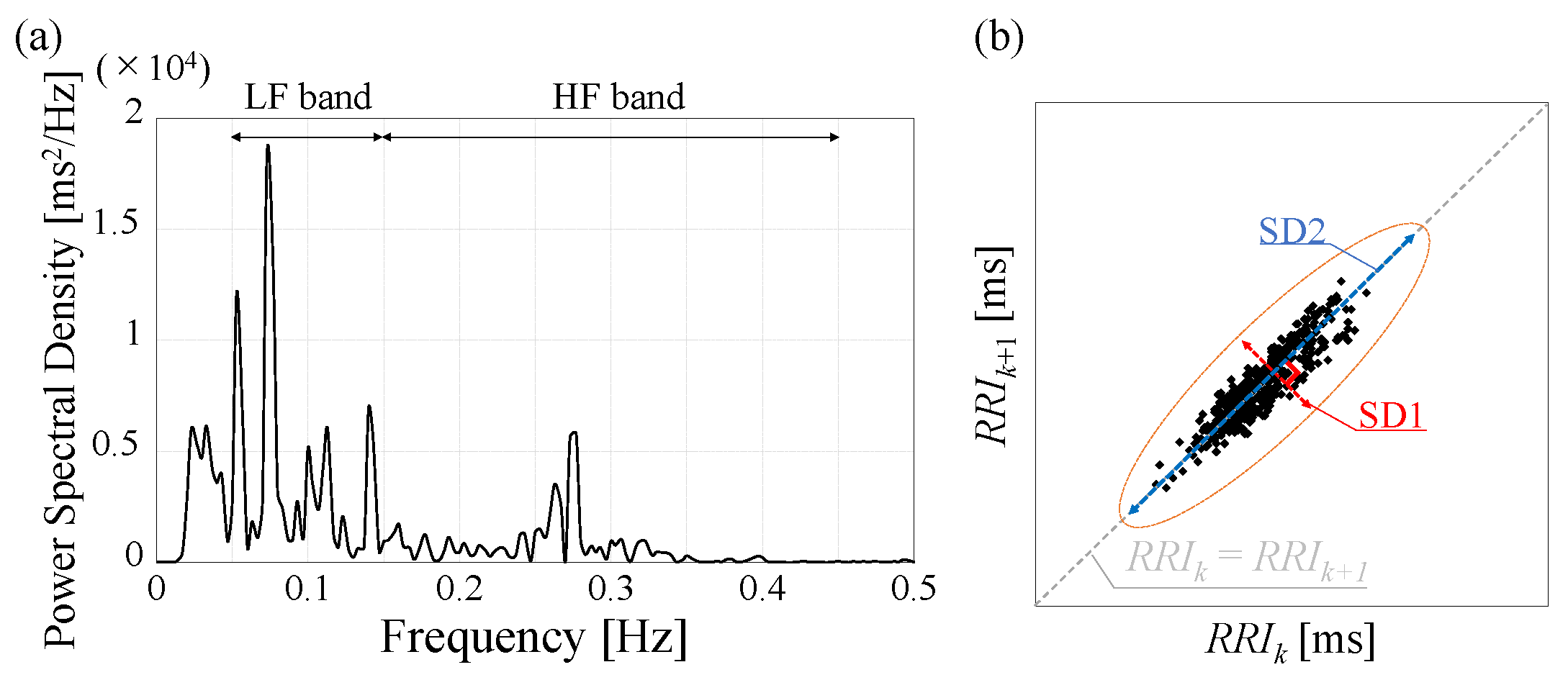
After the explanation of the experiment, an EEG (OpenBCI, Ultracortex Mark IV, Figure 2b) was attached to the subject’s head. In addition, a heart rate monitor (AffordSENS Corporation, Vitalgram, Figure 2c, Yokohama, Kanagawa, Japan) was attached to the chest. The hardware specifications for (b) and (c) are indicated as follows: The above EEG consists of the Cyton biosensing board (OpenBCI Inc., Brooklyn, NY, USA) and the the Ultracortex Mark IV EEG headset. The performance of the Cyton board is comparable to medical-grade EEG-amplifiers [26]. The specifications of the OpenBCI Cyton are listed in Table 1a. On the other hand, the above heart rate monitor, Vitalgram is a wearable adhesive plaster-type wireless biometric sensor. The specifications of this device are listed in Table 1b.
The sampling rate of the EEG was set to 250 Hz. The measured data were transmitted via Bluetooth and recorded. Figure 2d shows the monitoring points of the EEG. The sampling rate of the heart rate monitor was 512 Hz. The measured data were transmitted via Bluetooth and recorded as in the EEG. There were three types of EEG indices, α-EEG, β-EEG, and percent α-EEG (the ratio of α-EEG power within the sum of α- and β-EEG power), and two types of heart rate indices, the low-frequency component/high-frequency component (LF/HF) [27,28] and the standard difference 2/standard deviation 1 (SD2/SD1) [29,30], were used to evaluate biological responses. The EEG data used in the analysis were measured at the point of Pz on the parietal region of the head, as shown in Figure 2d. This is because the distribution of α-waves on the scalp has the maximum amplitude in the parietal and posterior regions [31]. Note that the reference electrode was attached to the earlobe to derive EEG based on the monopolar derivation method [32].

2.3. Analysis

The analysis methods of HRV and EEG are described as follows: Firstly, the raw data obtained using biological responses are not useful for comparison between different conditions since the absolute values of the brain waves and heart rates vary in each measurement. Therefore, we used the ratio of each biological parameter Bstimul measured at the time of stimulation to that of Brest during the pre-rest period before the presentation of the auditory stimuli, that is, the change rate R of each index calculated as per Equation (1) below:
R = B stim B rest B rest · 100
Finally, the change rates of α-EEG, β-EEG, percent α-EEG, LF/HF, and SD2/SD1 were treated as physiological parameters.
Next, the scheme of analysis for brain waves and heart rate is described hereafter. First, brain waves were analyzed as follows: The higher-frequency components were filtered out using a low-pass filter with frequency components up to 30 Hz. The unnecessary pulsive waves of artifacts caused by eye movements were manually detected and excluded. After this, the waveform was cut into multiple segments with a duration of 10 s, and the band-limited powers from f1 Hz to f2 Hz, Pf1−f2, of each segment in the α-band from 8 to 13 Hz and β-band from 13 to 30 Hz were calculated as per Equation (2) below:
P f 1 f 2 = f 1 f 2 P S D ( f ) d f ,
where PSD(f) is the power spectrum density obtained from the fast Fourier transform (FFT) treatment of each segment, and f1 and f2 are assigned as 8 Hz < f < 13 Hz for α-band and 13 Hz < f < 30 Hz for β-band, respectively.
Secondly, the HRV indices were analyzed by following the method indicated in Figure 3. First, the time intervals between each of the R-waves among each of the P, Q, R, S, T and U waves [33] were analyzed as a time series of the R-R interval (RRI) [34] from the waveform of the heart rate. Second, two kinds of heart rate indices of LF/HF and SD2/SD1 were adopted. LF/HF is an index for estimating sympathetic and parasympathetic activities [35] from the power spectrum of the RRI, while SD2/SD1 represents the RRI fluctuation that can be estimated based on the Poincaré plot [36], which is a geometric representation of the time series of RRIs.
LF/HF can be calculated from the energy ratio of LF (from 0.04 Hz to 0.15 Hz) of the time series of RRI to HF (from 0.15 Hz to 0.40 Hz). This parameter was calculated using the power spectrum obtained by FFT treatment. An example of the power spectrum is shown in Figure 4a. SD2/SD1 can be calculated as follows: By using the obtained time series of RRI, a Poincaré plot can be firstly obtained by plotting RRI at k th time step (RRIk) on the horizontal axis, while plotting RRI at k + 1 th time step (RRIk+1) on the vertical axis, as shown in Figure 4b. Then, SD2/SD1 can be calculated using the SD1 and SD2 of the Poincaré plot. Note that SD1 and SD2 are standard deviations of the plotted data in the orthogonal short and long axes of the ellipse, as shown in Figure 4b.

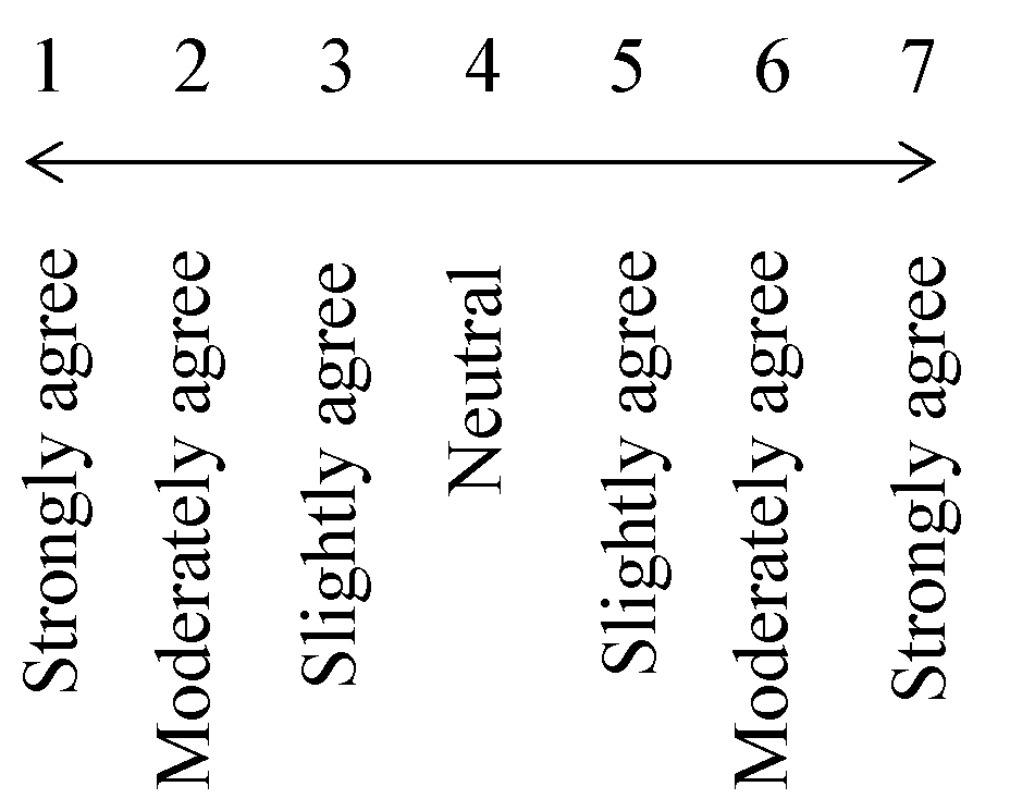
2.4. Subjective Evaluation Experiment

A subjective evaluation experiment was conducted to examine how each of the subjects perceived the same sounds. To measure the subjective human response to sound, various investigations have been conducted [37,38,39,40]. For example, the quality of various spaces such as room-acoustic spaces [37] and waterfront exterior spaces [38,39] are treated using psychological evaluations with subjective experiments. The relationship between the unpleasantness and tonality of sound has also been assessed using subjective evaluations. The room-acoustic impression is evaluated by using contrasting adjective pairs on a bipolar six-point semantic scale. Such an evaluation scheme is called an SD method, which was first introduced by Osgood [41]. This method is advantageous because of its easy-to-understand scaling and usage of popular adjectives. So, in the experiment, the SD method was used to evaluate subjective sound impressions.
Many studies have used this method. For example, Yamada et al. used it [42] to specify the subjective and objective effects of dental drill sounds on subjects. Like this study, the subjects were asked about their impression of the sound based on 15 paired adjectives. To evaluate the auditory impression of the contrasting sounds of white noise and murmuring river sound, 15 pairs of bipolar adjectives were selected: beautiful–dirty; clear–dull; comfortable–uncomfortable; smooth–rough; moist–dry; sentimental–unsentimental; powerful–powerless; rich–poor; noisy–quiet; large–small; loud–calm; metallic–not metallic; high pitched–low pitched; hard–soft; and bright–dark. Using the selected 15 pairs of adjective attributes, respondents rated each of the auditory stimuli on a bipolar seven-point semantic scale according to ISO 10551:1995 [43]. It should be noted that there was the option to use a unipolar 11-point scale according to ISO 15666:2003 [44]. However, in this study, it was preferable to use a bipolar scale for the bipolar adjectives above. Additionally, it is noted in [45] that the degree of relative differentiation based on indoor physical factors made no significant difference across these two response scales. In addition, in past studies, the bipolar seven-point semantic scale has been frequently used for auditory evaluation [42,46]. So, in this study, the bipolar seven-point scale was adopted as shown in Figure 5.

2.5. Statistical Analysis

The statistical analysis in this study was performed using R. In the analyses of the physiological indices and psychological scores, paired t-tests were used to compare the average values for the auditory stimulation periods between the murmuring river sound and white noise. For all the analyses, a p-value less than 0.05 was considered significant.

3. Results and Discussion

3.1. Profile Analysis

The results of the SD evaluation for each subject were arithmetically averaged and are summarized in Figure 6. The blue dots are the results for SA, while the orange dots are those for SB. There is a large difference between these two sounds. In particular, there are large differences in the rated scores for the items “beautiful”, “clear”, “pleasant”, “smooth”, and “bright”. As a result of the significance test for each evaluation factor, significant differences were found for all items (p < 0.05), indicating that the characteristic differences of the sounds affected the results of the subjective evaluation.

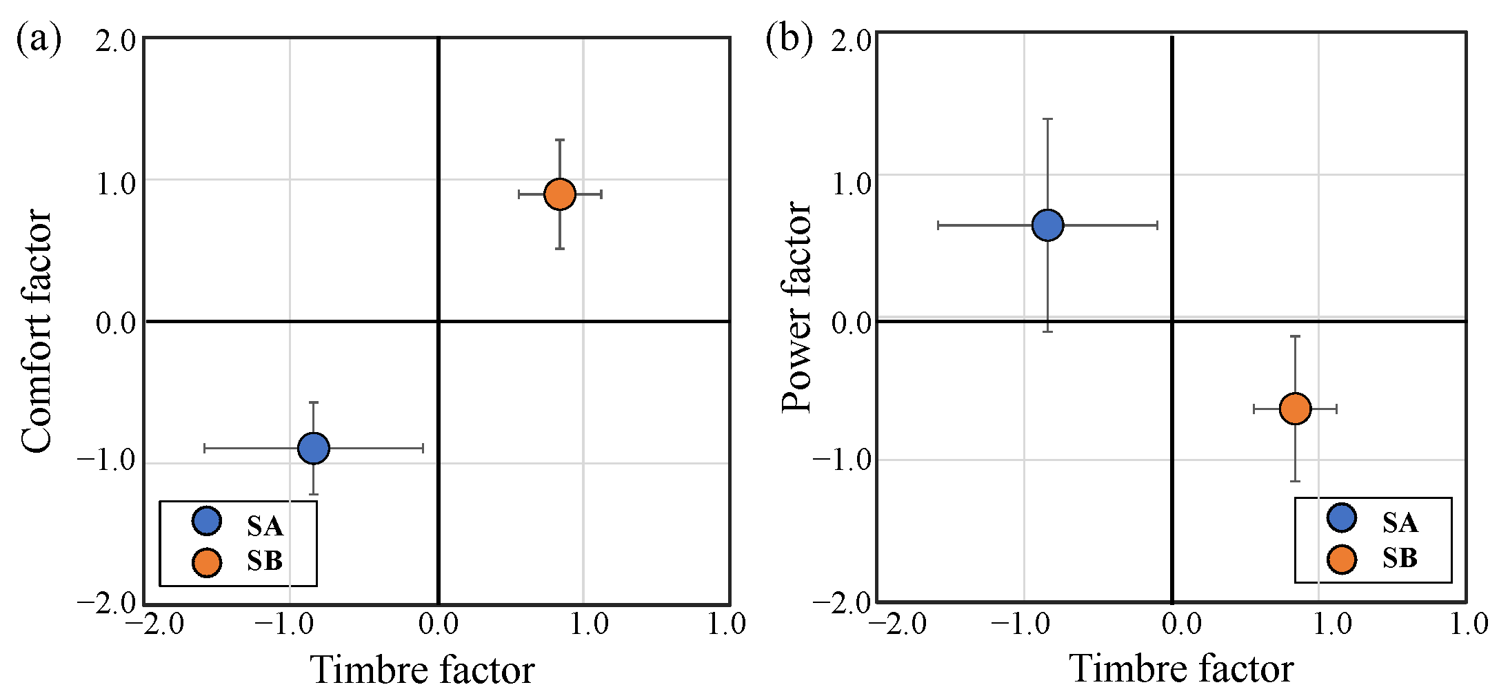
3.2. Factor Analysis

Factor analysis was conducted based on the maximum likelihood method with promax rotation. The number of factors was set at three by following the Kaiser–Guttman “Eigenvalues greater than one” criterion [47,48]. The factor loadings with the contribution ratio obtained from the analysis results are shown in Table 2. For each adjective, the factor with the highest factor loading is marked with a yellow marker. The factors were named as follows in consideration of the characteristics of their constituent items and their factor loadings: The first factor is the “comfort factor” and consists of “comfortable”, “beautiful”, “clear”, and “pleasant”. The second factor is the “timbre factor” and consists of “rich” and “metallic”. The third factor is the “power factor” and consists of “powerful” and “noisy”. The contribution rate of the comfort factor was the largest at 34%. From the cumulative contribution rate of all the factors, these three factors accounted for 80% of the contribution of all factors.
Figure 7a,b show the averaged factor scores and their SDs of the comfort and timbre factors (Figure 7a) and the power and timbre factors (Figure 7b), respectively. From these results, SB indicated a contrasting impression compared to SA, and was rated as a sound with a higher comfort score and lower timbre and power scores. Based on the above results, it can be suggested that white noise and murmuring river sounds can be separately perceived as uncomfortable and comfortable sounds, respectively, for the majority of people.

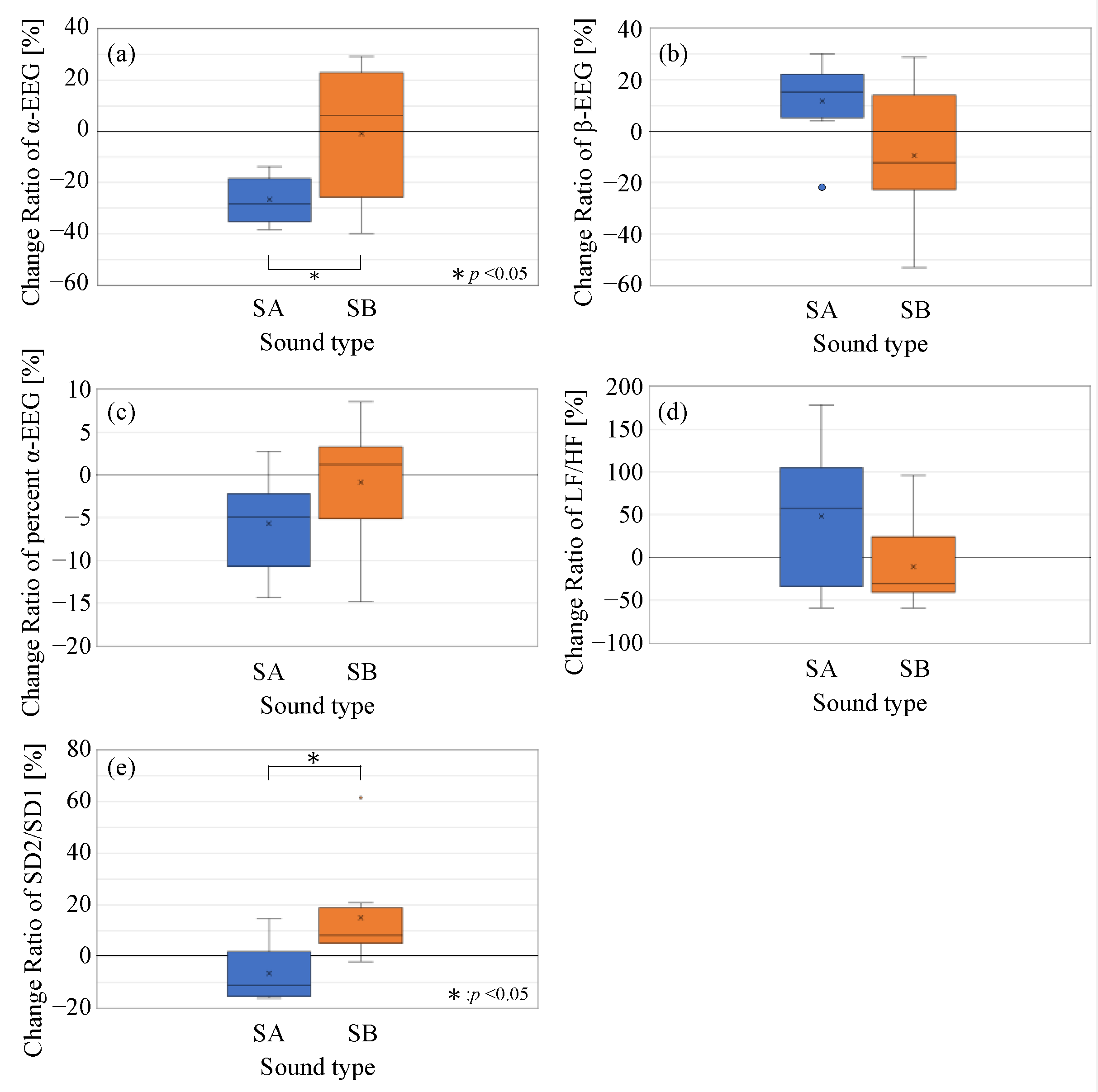
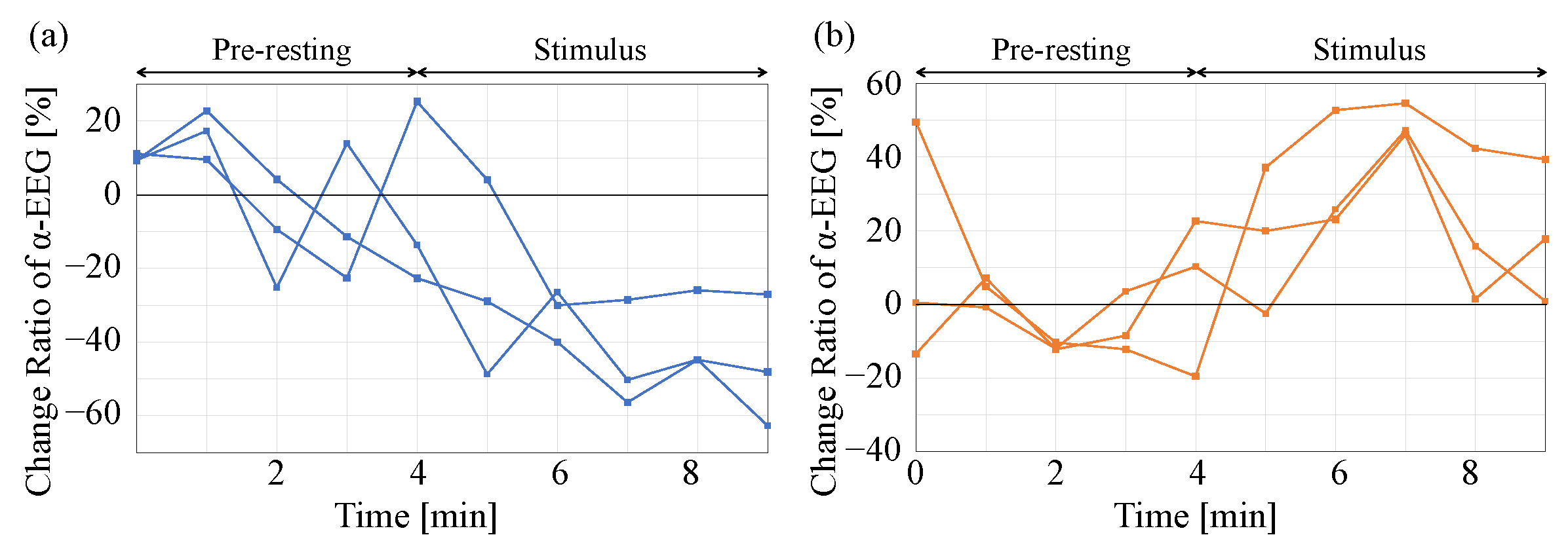
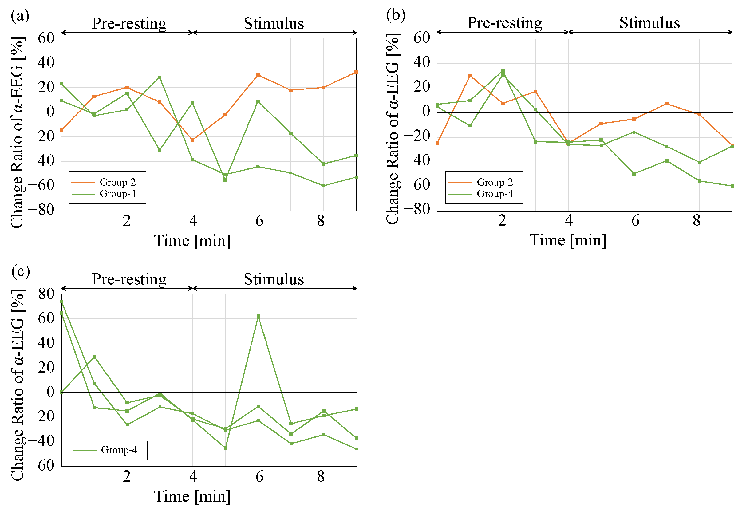
3.3. Physiological Response

The change rates of α-EEG, β- EEG, percent α-EEG, LF/HF, and SD2/SD1 are shown in Figure 8a–e, respectively. Note that, in this section, the biological data obtained from all three trials in Figure 1b are averaged and discussed. The change rates of α-EEG showed a significant difference between SA and SB (p < 0.05). This indicates that the α-EEG significantly decreased when SA was presented, while the α-EEG did not significantly increase when SB was presented. This is consistent with past research [49], where the brain wave in the alpha domain was also decreased by exposure to white noise. In some references, such as [50], the strength of α-waves was proportional to the degree of relaxation of the subject. However, in this study, the averaged result of α-EEG was not increased by the murmuring river sound. The reason for the unchanged α-EEG will be discussed in the next section. In the case of change rates of β-EEG and percent α-EEG, there was no significant difference between those in the SA and SB conditions. The presence of stress has been shown to increase the β-EEG [51], but in this case, it is considered that the environmental stress on humans caused by the white noise and murmuring river sound did not have different influences on human, while the α-EEG slightly increased in the SA condition. It is said that components in the beta frequency band are distributed in the front of the head [52], and the amount of frontal beta is correlated to task difficulty. The reason for the lack of a significant difference may be due to the fact that the stimulus was not a task involving difficult judgements, but rather just exposure to sounds. Moreover, in the literature [53], no significant differences have been observed between conditions with and without acoustic stimuli. However, the results of the present study had a greater standard deviation, especially under the SB condition, indicating large inter-individuality. This may be caused by inter-individual differences in the perception of the sound of a murmuring river.
Next, LF/HF slightly increased in the SA condition compared to the SB condition, but there was no significant difference between the conditions with and without acoustic stimuli. Since numerous papers have suggested that the increase in LF/HF is related to the increase in sympathetic nerve activity [28], the increase in LF/HF may be due to the stress that occurs when listening to uncomfortable sounds such as white noise. It is also related to previous results [54] where the HF component decreased with white noise exposure. SD2/SD1 showed a decreasing trend during the SA condition and an increasing trend during the SB condition, with a significant difference between the two sound sources (p < 0.05). It is said that SD2/SD1 is related to autonomic balance where SD2 reflects sympathetic cardiac regulation and SD1 reflects parasympathetic activity [55,56]. In addition, in yet another study [57], it is shown that when white noise is greater 50 dBA, significant sympathetic activation is induced, producing significant cardiovascular stress. Thus, it may be reasonable that SD2/SD1 decreased with white noise exposure and increased with exposure to the more comfortable murmuring river sound.
Herein, both α-EEG and SD2/SD1 decreased in the white noise condition, while increased or unchanged in the murmuring river sound condition. So, the correlations between (a) α-EEG and SD2/SD1 and (b) β-EEG and SD2/SD1 are shown in Figure 9a,b, respectively. As shown in Figure 9a, the SD2/SD1 increases as the α-EEG increases, while, in Figure 9b, the SD2/SD1 decreases as the β-EEG increases. So, it can be estimated that the physiological parameters related to HRV and EEG could be correlated with each other.
In the above physiological responses, it can been seen that large variations generally occurred in all results of the present study. In the literature, it has also been pointed out that α-EEG was more largely induced by preferred musical stimulation than non-preferred [15]. This may be influenced by differences in the way individuals subjectively perceive sound. In the next section, the correspondence of the results with those of the subjective evaluation experiment will be discussed.

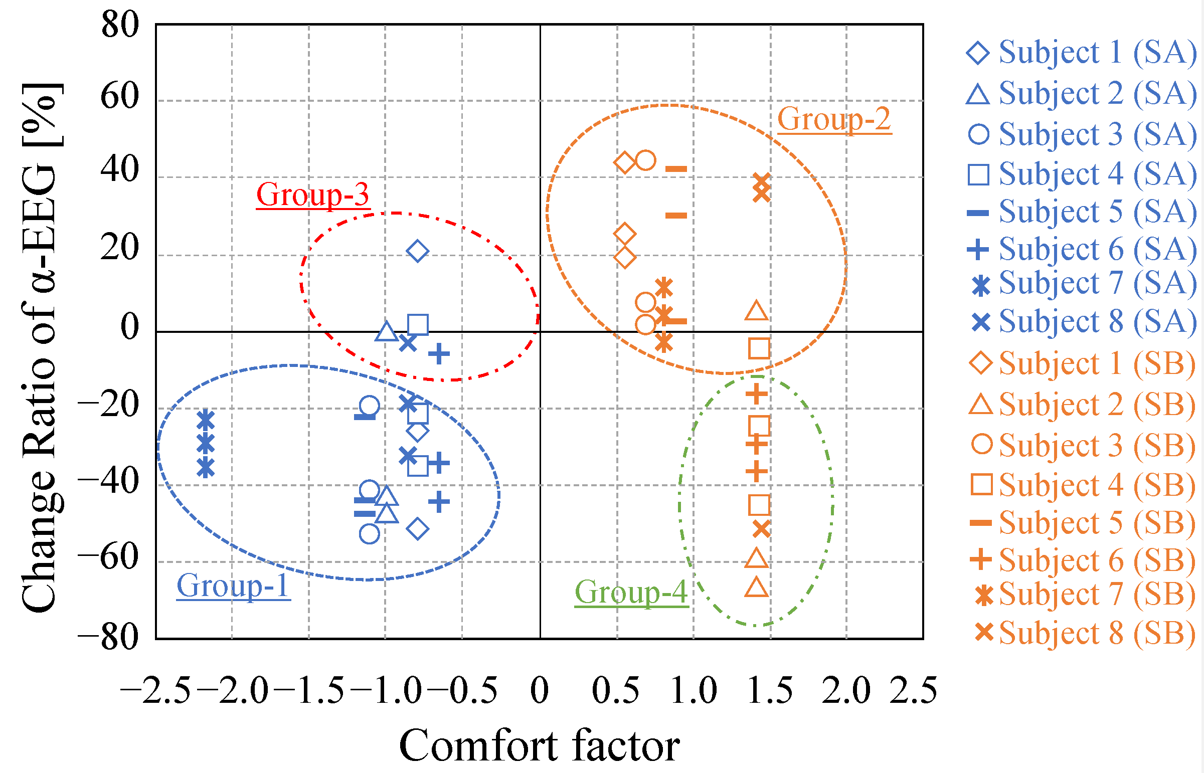
3.4. Relationship between Subjective and Biological Responses

To examine the relationship between subjective and biological responses, the relationship between the factor scores of the subjective evaluation and the five indicators of biological response were discussed. First, the results of the correlation coefficients and their p values are shown in Table 3. The α-EEG was correlated with each subjective evaluation result. This suggests that the α-EEG is the indicator most highly correlated with the results of the subjective evaluation.
A non-hierarchical cluster analysis using the k-means method was conducted using the factor scores and the change rate of α-EEG, and the relationships among them were discussed for each cluster. The data used for the analysis consisted of two types of sound sources and three experiments with eight subjects, for a total of 48 datasets that were classified into four groups. The results of the cluster analysis are shown in Figure 10. The orange plots show the results when SB was presented, while the blue plots show those when SA was presented. Each marker indicates individual subjects. It should be noted that, in this figure, the subjective data were obtained only once for the three biological data. The results of the analysis were classified into the following four groups: Group-1, whose α-EEG decreased when presented with white noise; Group-2, whose α-EEG increased when presented with the murmuring river sound; Group-3, whose α-EEG did not change or increase when presented with white noise; and Group-4, whose α-EEG decreased when presented with the murmuring river sound. The differences among these groups were examined using the time trends of the change rate of α-EEG. The examples of the results measured during the three different trials for one subject marked by blue and orange circles in Groups-1 and 2 are shown in Figure 11a,b, respectively. These figures show that the α-EEG of the subject decreased by 4 to 9 min after the presentation of white noise (Figure 11a), while that in Group-2 increased by 4 to 9 min after the presentation of the murmuring river sound (Figure 11b).
Figure 12a–c show examples of subjects categorized into Group-4. From Figure 12a,b, it can be seen that the α-EEGs of the subjects with triangular and rectangular legends tended to decrease in two experiments, while they tended to increase in the remaining experiment when listening to the murmuring river sound. From Figure 12c, it can be seen that the α-EEG of the subject indicated by a plus sign tended to decrease in all three experiments when listening to the murmuring river sound. As shown in this figure, the majority of the subjects indicated decreased α-EEG in the SB condition, while the subjects indicated various α-EEG values depending on the individuals. The reason for these results may be due to the effects of other subjective factors of power, as described below.
Figure 13 shows the results of the relationship between α-EEG and the factor scores of power. In this figure, the three subjects surrounded by the broken lines felt power behind the murmuring river sound. From this result, it is shown that these three subjects felt a negative impression of the power associated with the murmuring river sound, which led to the decrease in α-EEG. This suggests that individuals have different mechanisms of subjective evaluation of comfort even when the same auditory stimulus is given, and that these different impressions have effects on biological responses.

4. Conclusions

The relationship between subjective and biological responses to acoustic stimuli with comfortable and uncomfortable sounds was investigated in this study. Compared with the murmuring river sound, white noise showed significantly decreased α-EEG and SD2/SD1. The correlation between each index of subjective and biological responses was examined. It was found that the α-EEG was highly correlated with the result of the subjective evaluation. However, when the subjects were divided into groups by cluster analysis, it was also seen that the α-EEG decreased in subjects who felt that the murmuring river sound was powerful, even though it is a natural sound. Furthermore, some subjects showed different biological responses in each trial, and it was suggested that biological responses may vary, and this was especially the case for the subject who felt that the sound was not comfortable but powerful.
The contents of this paper can be applied to the fields of product design, which requires psychological and physiological sound quality evaluations such as car cabin noise. By using such a method, where sound quality can be easily assessed by using physiological indicators, the evaluation of sound can be efficiently conducted. Additionally, comfortable sounds, such as water sounds, can be played in a noisy environment such as inside stations to make them more comfortable spaces.
In this study, the relationship between subjective and objective responses was investigated using two contrasting sounds in terms of whether the subjects perceived them as comfortable or not. However, since the characteristics of the environmental sounds largely varied, the obtained relationship between biological responses and subjective impressions will have to be expanded in future work by increasing the kinds of test sounds.

Funding

This research received no external funding.

Institutional Review Board Statement

Not applicable.

Informed Consent Statement

Informed consent was obtained from all subjects involved in the study.

Data Availability Statement

Not applicable.

Acknowledgments

The author would like to thank A. Nakamura for technical assistance with the subjective evaluation tests.

Conflicts of Interest

The author declares no conflict of interest.

References

  1. Cohen, S.; Kessler, R.C.; Gordon, L.U. Strategies for measuring stress in studies of psychiatric and physical disorders. In Measuring Stress: A Guide for Health and Social Scientists; Cohen, S., Kessler, R.C., Gordon, L.U., Eds.; Oxford University Press: Oxford, UK, 1995. [Google Scholar]
  2. Lampert, R. ECG signatures of psychological stress. J. Electrocardiol. 2015, 48, 1000–1005. [Google Scholar] [CrossRef] [PubMed] [Green Version]
  3. Blons, E.; Arsac, L.M.; Grivel, E.; Lespinet-Najib, V.; Deschodt-Arsac, V. Physiological resonance in empathic stress: Insights from nonlinear dynamics of heart rate variability. Int. J. Environ. Res. Public Health. 2021, 18, 2081. [Google Scholar] [CrossRef] [PubMed]
  4. Gordon, A.M.; Mendes, W.B. A large-scale study of stress, emotions, and blood pressure in daily life using a digital platform. Proc. Natl. Acad. Sci. USA 2021, 118, e2105573118. [Google Scholar] [CrossRef] [PubMed]
  5. Roger, A.D.; Lisete, C.M.; De-Pei, L.; Hui-Lin, P. Regulation of sympathetic vasomotor activity by the hypothalamic paraventricular nucleus in normotensive and hypertensive states. Am. J. Physiol. Heart Circulat. Phys. 2018, 315, H1200–H1214. [Google Scholar]
  6. Suess, W.M.; Alexander, A.B.; Smith, D.D.; Sweeney, H.W.; Marion, R.J. The Effects of Psychological Stress on Respiration: A Preliminary Study of Anxiety and Hyperventilation. Psychophysiology 1980, 17, 535–540. [Google Scholar] [CrossRef]
  7. Baker, L.M.; Taylor, W.M. The relationship under stress between changes in skin temperature, electrical skin resistance, and pulse rate. J. Exp. Psychol. 1954, 48, 361–366. [Google Scholar] [CrossRef]
  8. Blore, D. Use of eye movement to reduce stress after trauma. Nurs. Times 1996, 92, 43–45. [Google Scholar]
  9. Li, T.M.; Chao, H.C.; Zhang, J. Emotion classification based on brain wave: A survey. Hum. Cent. Comput. Inf. Sci. 2019, 9, 42. [Google Scholar] [CrossRef] [Green Version]
  10. Gerrard, P.; Malcolm, R. Mechanisms of modafinil: A review of current research. Neuropsychiatr. Dis. Treat. 2007, 3, 349–364. [Google Scholar] [PubMed]
  11. Haas, L.F. Hans Berger (1873–1941), Richard Caton (1842–1926), and electroencephalography. J. Neurol. Neurosurg. Psychiatry. 2003, 74, 9. [Google Scholar] [CrossRef] [Green Version]
  12. Jang, E.H.; Byun, S.; Park, M.S.; Park, J.H. Reliability of Physiological Responses Induced by Basic Emotions: A Pilot Study. J. Physiol. Anthropol. 2019, 38, 15. [Google Scholar] [CrossRef] [PubMed]
  13. Thoma, M.V.; Mewes, R.; Nater, U.M. Preliminary evidence: The stress-reducing effect of listening to water sounds depends on somatic complaints: A randomized trial. Medicine 2018, 97, e9851. [Google Scholar] [CrossRef] [PubMed]
  14. Koelsch, S.; Walter, A.S. Towards a neural basis of music perception. Trends Cogn. Sci. 2005, 9, 578–584. [Google Scholar] [CrossRef] [PubMed] [Green Version]
  15. Gentry, H.; Humphries, E.; Peña, S.; Mekic, A.; Hurless, N.; Nichols, D.F. Music genre preference and tempo alter alpha and beta waves in human non-musicians. Impuls. Prem. Undergrad. Neurosci. J. 2013, 22, 1–11. [Google Scholar]
  16. Norbert, J.; Katarina, H. The influence of Mozart sonata K.448 on brain activity during the performance of spiritual rotation and numerical tasks. Brain Topogr. 2005, 17, 207–218. [Google Scholar]
  17. Caldwell, G.N.; Riby, L.M. The effects of music exposure and own genre preference on conscious and unconscious cognitive processes: A pilot ERP study. Conscious. Cogn. 2007, 16, 992–996. [Google Scholar] [CrossRef]
  18. Park, S.A.; Song, C.; Choi, J.Y.; Son, K.C.; Miyazaki, Y. Foliage Plants cause physiological and psychological relaxation as evidenced by measurements of prefrontal cortex activity and profile of mood states. HortScience 2016, 51, 1308–1312. [Google Scholar] [CrossRef]
  19. Acharya, R.; Joseph, P.; Kannathal, N.; Lim, C.M.; Suri, J. Heart rate variability: A review. Med. Biol. Eng. Comput. 2006, 44, 1031–1051. [Google Scholar] [CrossRef]
  20. Kim, H.-G.; Cheon, E.-J.; Bai, D.-S.; Lee, Y.H.; Koo, B.-H. Stress and heart rate variability: A meta-analysis and review of the literature. Psychiatry Investig. 2018, 15, 235–245. [Google Scholar] [CrossRef] [Green Version]
  21. Vicente, J.; Laguna, P.; Bartra, A.; Bailón, R. Drowsiness detection using heart rate variability. Med. Biol. Eng. Comput. 2016, 54, 927–937. [Google Scholar] [CrossRef]
  22. Spangler, D.; Alam, S.; Rahman, S.; Crone, J.; Robucci, R.; Banerjee, N.; Kerick, S.; Brooks, J. Multilevel longitudinal analysis of shooting performance as a function of stress and cardiovascular responses. IEEE Trans. Affect. Comput. 2020, 12, 648–665. [Google Scholar] [CrossRef]
  23. Fukuba, Y.; Sato, H.; Sakiyama, T.; Endo, Y.M.; Yamada, M.; Ueoka, H.; Miura, A.; Koga, S. Autonomic nervous activities assessed by heart rate variability in pre- and post-adolescent Japanese. J. Physiol. Anthropol. 2009, 28, 269–273. [Google Scholar] [CrossRef] [PubMed] [Green Version]
  24. Guzmán, A.; Jaime, V.; Beatriz, R.; Pedro, M.; Ángel, M.M. The relationship between heart rate variability and electroencephalography functional connectivity variability is associated with cognitive flexibility. Front. Hum. Neurosci. 2019, 13, 64. [Google Scholar]
  25. Piper, D.; Schiecke, K.; Leistritz, L.; Pester, B.; Benninger, F.; Feucht, M.; Ungureanu, G.; Strungaru, R.; Witte, H. Synchronization analysis between heart rate variability and EEG activity before, during, and after epileptic seizure. Biomed. Eng. 2014, 59, 343–355. [Google Scholar] [CrossRef] [PubMed]
  26. Frey, J. Comparison of an open-hardware electroencephalography amplifier with medical grade device in brain-computer interface applications. arXiv 2016, arXiv:1606.02438. [Google Scholar]
  27. Perini, R.; Veicsteinas, A. Heart rate variability and autonomic activity at rest and during exercise in various physiological conditions. Eur. J. Appl. Physiol. 2003, 90, 317–325. [Google Scholar] [CrossRef] [PubMed]
  28. Kleiger, R.E.; Stein, P.K.; Bigger, J.T., Jr. Heart rate variability: Measurement and clinical utility. Ann. Noninvasive Electrocardiol. 2005, 10, 88–101. [Google Scholar] [CrossRef]
  29. Guzik, P.; Piskorski, J.; Krauze, T.; Schneider, R.; Wesseling, K.H.; Wykretowicz, A.; Wysocki, H. Correlations between the Poincaré plot and conventional heart rate variability parameters assessed during paced breathing. J. Physiol. Sci. 2007, 57, 63–71. [Google Scholar] [CrossRef] [Green Version]
  30. Behbahani, S.; Dabanloo, N.J.; Nasrabadi, A.M. Ictal heart rate variability assessment with focus on secondary generalized and complex partial epileptic seizures. Adv. Biores. 2012, 4, 50–58. [Google Scholar]
  31. Brigo, F.; Ausserer, H.; Nardone, R.; Tezzon, F.; Manganotti, P.; Bongiovann, L.G. Subclinical rhythmic electroencephalogram discharge of adults occurring during sleep: A diagnostic challenge. Clin. EEG Neurosci. 2013, 44, 227–231. [Google Scholar] [CrossRef]
  32. Sorel, L.; Ranwez, R. Basis and use of a true monopolar derivation: The neo-electroencephalography (N.E.E.G.). Clin. Electroencephalogr. 1984, 15, 71–82. [Google Scholar] [CrossRef] [PubMed]
  33. Hurst, J.W. Naming of the waves in the ECG, with a brief account of their genesis. Circulation 1998, 98, 1937–1942. [Google Scholar] [CrossRef] [PubMed] [Green Version]
  34. Peltola, M.A. Role of editing of R-R intervals in the analysis of heart rate variability. Front. Physiol. 2012, 3, 148. [Google Scholar] [CrossRef] [Green Version]
  35. Camm, J. Task force of the European Society of Cardiology the North American Society of Pacing Electrophysiology; Heart rate variability: Standards of measurement, physiological interpretation and clinical use. Circulation 1996, 93, 1043–1065. [Google Scholar]
  36. Wheeler, T.; Watkins, P.J. Cardiac denervation in diabetes. BMJ 1973, 4, 584–586. [Google Scholar] [CrossRef] [PubMed] [Green Version]
  37. Farina, A. Acoustic quality of theatres: Correlations between experimental measures and subjective evaluations. Appl. Acoust. 2001, 62, 889–916. [Google Scholar] [CrossRef]
  38. Romero, V.P.; Maffei, L.; Brambilla, G.; Ciaburro, G. Modelling the soundscape quality of urban waterfronts by artificial neural networks. Appl. Acoust. 2016, 111, 121–128. [Google Scholar] [CrossRef]
  39. Puyana Romero, V.; Maffei, L.; Brambilla, G.; Ciaburro, G. Acoustic, visual and spatial indicators for the description of the soundscape of waterfront areas with and without road traffic flow. Int. J. Environ. Res. Public Health 2016, 13, 934. [Google Scholar] [CrossRef]
  40. Parizet, E.; Bolmont, A.; Fingerhuth, S. Subjective evaluation of tonalness and relation between tonalness and unpleasantness. In INTER-NOISE and NOISE-CON Congress and Conference Proceedings; Institute of Noise Control Engineering: Washington, DC, USA, 2009; Volume 2009, pp. 934–941. [Google Scholar]
  41. Osgood, C.E.; Tzeng, O. Language, Meaning, and Culture: The Selected Papers of C.E. Osgood; Praeger Publishers: Westport, CT, USA, 1990. [Google Scholar]
  42. Yamada, T.; Kuwano, S.; Ebisu, S.; Hayashi, M. Statistical analysis for subjective and objective evaluations of dental drill sounds. PLoS ONE 2016, 11, e0159926. [Google Scholar] [CrossRef]
  43. ISO 10551; Ergonomics of the Thermal Environment—Assessment of the Influence of the Thermal Environment Using Subjective Judgement Scales. ISO: Geneva, Switzerland, 1995.
  44. ISO/TS 15666; Acoustics—Assessment of Noise Annoyance by Means of Social and Socio-Acoustic Surveys. ISO: Geneva, Switzerland, 2003.
  45. Yang, W.; Moon, H.J.; Jeon, J.Y. Comparison of Response Scales as Measures of Indoor Environmental Perception in Combined Thermal and Acoustic Conditions. Sustainability 2019, 11, 3975. [Google Scholar] [CrossRef] [Green Version]
  46. Hong, J.Y.; Jeon, J.Y. Designing sound and visual components for enhancement of urban soundscapes. J. Acoust. Soc. Am. 2013, 134, 2026–2036. [Google Scholar] [CrossRef] [PubMed]
  47. Guttman, L. A new approach to factor analysis: The Radex. In Mathematical Thinking in the Social Sciences; Lazarsfeld, P.F., Ed.; Free Press: New York, NY, USA, 1954; pp. 258–348. [Google Scholar]
  48. Kaiser, H.F. The application of electronic computers to factor analysis. Educ. Psychol. Meas. 1960, 20, 141–151. [Google Scholar] [CrossRef]
  49. Saito, K. Effect of noise on higher nervous activity. J. Sound Vib. 1988, 127, 419–424. [Google Scholar] [CrossRef]
  50. Matsui, K.; Kawai, J.; Sawamura, K.; Kohara, Y.; Matsumoto, K. A psychophysiological study on biological reaction using music stimuli. J. Clin. Educ. Psychol. 2003, 29, 43–57. [Google Scholar]
  51. Hamid, N.H.A.; Sulaiman, N.; Murat, Z.H.; Taib, M.N. Brainwaves stress pattern based on perceived stress scale test. In Proceedings of the IEEE 6th Control and System Graduate Research Colloquium, Shah Alam, Malaysia, 10–11 August 2015; pp. 135–140. [Google Scholar]
  52. Kropotov, J.D. Quantitative EEG, Event-Related Potentials and Neurotherapy, 1st ed.; Academic Press: Moscow, Russia, 2010. [Google Scholar]
  53. Nishifuji, S.; Sato, M.; Maino, D.; Tanaka, S. Effect of acoustic stimuli and mental task on alpha, beta and gamma rhythms in brain wave. In Proceedings of the SICE Annual Conference 2010, Taipei, Taiwan, 18–21 August 2010; pp. 1548–1554. [Google Scholar]
  54. Roque, A.; Valenti, V.; Guida, H.; Campos, M.; Knap, A.; Vanderlei, L.; Ferreira, L.; Ferreira, C.; Abreu, L. The effects of auditory stimulation with music on heart rate variability in healthy women. Clinics 2013, 68, 960–967. [Google Scholar] [CrossRef]
  55. Toichi, M.; Sugiura, T.; Murai, T.; Sengoku, A. A new method of assessing cardiac autonomic function and its comparison with spectral analysis and coefficient of variation of R–R interval. J. Auton. Nerv. Syst. 1997, 62, 79–84. [Google Scholar] [CrossRef]
  56. Tulppo, M.P.; Mäkikallio, T.H.; Takala, T.E.; Seppänen, T.; Huikuri, H.V. Quantitative beat-to-beat analysis of heart rate dynamics during exercise. Am. J. Physiol. 1996, 271, 244–252. [Google Scholar] [CrossRef]
  57. Lee, G.S.; Chen, M.L.; Wang, G.Y. Evoked response of heart rate variability using short-duration white noise. Auton. Neurosci. 2010, 155, 94–97. [Google Scholar] [CrossRef]
Figure 1. Experimental processes (a) for each of the trials and (b) for the entire experiment.
Applsci 12 03417 g001
Figure 2. (a) Experimental environment inside the dark room, (b) adopted EEG headset (OpenBCI, Ultracortex Mark IV), (c) heart rate monitor (AffordSENS Corporation, Vitalgram), and (d) electrode arrangement points.
Applsci 12 03417 g002
Figure 3. Flow chart of analysis of HRV.
Applsci 12 03417 g003
Figure 4. Examples of (a) power spectral density and (b) Poincaré plot, respectively.
Applsci 12 03417 g004
Figure 5. Seven-point scale adopted in the subjective evaluation experiment.
Applsci 12 03417 g005
Figure 6. Results of the profile analysis of the subjective evaluation experiment. All the results for each of the subjects were arithmetically averaged and as a profile. The blue dots are the results for SA, while the orange dots are those for SB. There is a large difference between these two sounds with significant differences for all items (p < 0.05).
Applsci 12 03417 g006
Figure 7. Relationship of the averaged factor scores and SDs between (a) beauty and timbre factors, and (b) timbre and power factors, respectively. These scores of SA (white noise) and SB (murmuring river sound) contrast with each other, and white noise and murmuring river sounds can be separately perceived as uncomfortable and comfortable sounds.
Applsci 12 03417 g007
Figure 8. Experimental results of the averaged values and their SDs of the biological responses of (a) α-EEG, (b) β-EEG, (c) percent α-EEG, (d) LF/HF, and (e) SD2/SD1, respectively. In these results, each of the biological results in the conditions of SA (white noise) and SB (murmuring river sound) are shown. The asterisk shows a significant difference between SA and SB (p < 0.05).
Applsci 12 03417 g008
Figure 9. Relationship between (a) α-EEG and SD2/SD1 and (b) β-EEG and SD2/SD1, respectively.
Applsci 12 03417 g009
Figure 10. Results of the non-hierarchical cluster analysis by the k-means method. Blue plots indicate scores for SA (white noise), while orange plots indicate scores for SB (murmuring river sound). Each marker indicates an individual subject. All 48 data including two types of sound sources (SA and SB) and three experiments with eight subjects were classified into Group-1 to Group-4.
Applsci 12 03417 g010
Figure 11. Examples of the time-transient change rate of α-EEG of (a) one subject indicated by blue minus signs (Subject 5, Figure 9) categorized into Group-1 with white noise, and (b) one subject indicated by minus signs (Subject 5, Figure 9) categorized into Group-2 with murmuring river sound, respectively. In these time-transient waveforms, the initial four minutes are for the pre-resting time without any sound reproduction, while the latter five minutes are for the time of sound reproduction. Note that in these figures the three trials in the experiment are indicated as three lines. In these results, the α-EEG of the subject decreased by 4 to 9 min after the presentation of white noise in (a), while increased by 4 to 9 min after the presentation of the murmuring river sound in (b).
Applsci 12 03417 g011
Figure 12. Examples of the time-transient change rate of α-EEG of (a) one subject indicated by orange triangles (Subject 2, Figure 9) categorized into both Group-2 and -4 with murmuring river sound, (b) another subject indicated by orange squares (Subject 4, Figure 9) categorized into both Group-2 and -4 with murmuring river sound and (c) another subject indicated by orange plus signs (Subject 6, Figure 9) categorized into only Group-4 with murmuring river sound, respectively. Note that in these figures the three trials in the experiment are indicated as three lines. In the case of subject in (c), all three lines indicate decreased α-EEG, while in the cases of (a,b), one line indicates increased α-EEG compared to the other two lines, indicating decreased α-EEG.
Applsci 12 03417 g012
Figure 13. Relationship between the change ratio of α-EEG and the factor scores of power. Each marker indicates the same subjects as those in Figure 9. Each odatum includes two types of sound sources (SA and SB) and three experiments with eight subjects. Blue plots indicate scores for SA (white noise), while orange plots indicate scores for SB (murmuring river sound).
Applsci 12 03417 g013
Table 1. Hardware specifications for (a) Ultracortex Mark IV (OpenBCI Inc., Brooklyn, NY, USA), and (b) Vitalgram (AffordSENS Corporation, Vitalgram, Figure 2c, Yokohama, Kanagawa, Japan), respectively.
(a)
Channels8
Quantization bit rate24-bit
Possible gain1, 2, 4, 6, 8, 12, 24
Operation voltage3.3 V
AmplifierTexas Instruments ADS1299 ADC
MicrocontrollerPIC32MX250F128B
(b)
Sampling frequency128, 256, 512, 1024 Hz
Quantization bit rate10-bit
Radio communicationBluetooth 4.0 wireless technology
Power supplyRechargeable Li-ion battery
Terminal OSiOS 8.0 and above
Table 2. Results of the factor loadings and the contribution ratio of the 15 adjectives for each factor of factors 1, 2 and 3 obtained from the factor analysis. For each adjective, the factor with the highest factor loading is marked with a yellow marker. The first, second and third factors are named the “comfort factor”, “timbre factor” and “power factor”, respectively. The contribution rate of the comfort factor was the largest at 34%.
Factor 1Factor 2Factor 3
Beautiful-Dirty0.780.18−0.13
Clear-Dull0.730.16−0.19
Comfortable-Uncomfortable0.550.32−0.24
Smooth-Rough1.12−0.35−0.14
Unsentimental-Sentimental−0.43−0.24−0.37
Loud-Calm−0.74−0.210.05
Bright-Dark0.430.38−0.18
Low-pitched-High-pitched0.470.320.38
Moist-Dry0.450.48−0.17
Poor-Rich0.01−0.70−0.07
Large-Small0.100.81−0.04
Soft-Hard0.210.67−0.07
Metallic-Not metallic−0.23−0.70−0.49
Powerless-Powerful−0.120.13−0.87
Quiet-Noisy0.12−0.42−0.69
Contribution ratio0.340.280.18
Cumulative contribution ratio0.340.620.80
Table 3. Correlation coefficient between each subjective score and each biological parameter and p values of each correlation. Among each of the biological parameters, the α-EEG was mostly correlated with each subjective evaluation result. (*; p < 0.05, **; p < 0.1).
Comfort FactorTimbre FactorPower Factor
Corr. Coeff.p ValueCorr. Coeff.p ValueCorr. Coeff.p Value
a-EEG0.480.05*−0.560.02*0.520.04*
b-EEG0.400.12 −0.540.03*−0.370.15
Percent a-EEG0.240.36 −0.210.43 −0.430.03*
LF/HF−0.440.09**0.370.16 0.400.13
SD2/SD10.440.09**−0.580.02*−0.330.21
Publisher’s Note: MDPI stays neutral with regard to jurisdictional claims in published maps and institutional affiliations.

