URANS Analysis of a Launch Vehicle Aero-Acoustic Environment

Abstract

Predicting and mitigating acoustic levels become critical because of the harsh acoustic environment during space vehicle lift-off. This paper aimed to study the aero-acoustic environment during a rocket lift-off. The sound propagation within a launch event was studied using dedicated computational fluid dynamics (CFD). The resolution of all the phenomena that occur is unfeasible. We discuss the turbulence simplification and propose a feasible simulation through an unsteady Reynolds-averaged Navier–Stokes (URANS) model. The results were validated with experimental data showing a good correlation near the fairing surface and an improvable accuracy in the far field. To assess noise generation, the main shock waves were identified, and the evolution of the generated sound pressure was assessed. Moreover, vertical directivity was revealed by data analysis of the pressure field surrounding the fairing.

1. Introduction

The acoustic conditions during spacecraft launch are highly complex. The exhaust gas jet of the rocket engine and its collision with the launchpad produce severe acoustic waves, which are the primary sound sources during lift-off [1,2]. This acoustic environment causes a severe acoustic and vibration load on the payload, endangering the mission and potentially resulting in financial losses [3]. Hence, predicting and mitigating acoustic levels during lift-off are critical in the launch pad and launch vehicle design since this enhances the reliability of the launcher while also increasing payload comfort.

This work is part of a project, conducted under a European Space Agency (ESA) program, to develop a sound mitigation system applicable to the launch facility of the VEGA rocket. The first step towards any mitigation process is the prediction of noise sources. The global study of sound generation and transmission up to the payload entails several problems of different natures, which are summarized in Figure 1a. First, sound generation is mainly due to the exhaust gases’ jet with the blast wave generated during ignition. As shown in Figure 1b, the noise generated by the jet comprises three distinct sound sources: turbulent mixing noise (TMN), shock-associated noise (SAN), and impinging tones. The TMN is generated by the turbulent mixing of large-scale or small-scale eddies at the mixing layer [2,4]. Large-scale vortex noise dominates at supersonic speeds, resulting in low-frequency noise with high downstream directivity, as the blue arrows represent in Figure 1b [5]. The SAN in impinging jets is produced by the interaction of turbulent structures with shock waves, and it is called broadband shock-associated noise (BBSAN). The BBSAN is broadband and primarily directed upstream, as the green arrows represent, where the launch vehicle is located. Finally, the impinging tones appear when the jet collides and are directed upstream [2]. Second, there is an air transmission of these noise sources, which interact with the launchpad and are redirected to the vehicle. Thirdly, blast wave noise is also transmitted through the launcher structure up to the fairing and payload base. Finally, the structural vibration of the fairing interacts with the airborne noise in a vibroacoustic problem.

This work aimed to analyze the sound sources and their propagation during the lift-off stage. The approach here was to use computational fluid dynamics (CFD) to resolve the aero-acoustic problem that includes the study of the engine exhaust jet and its interaction with the launch pad. The simulation of all the physical phenomena that occur during the launch of rockets, such as exhaust gases’ combustion, supersonic flow compressibility, and lift of the launch vehicle, is unfeasible. Solving the generated turbulence with a sufficient resolution requires a direct numerical simulation in a vast domain [6]. There is currently not enough computational power to achieve this. This lack of resources forces making simplifications, as done in the literature [7,8]. Within these simplifications, it is fundamentally under discussion up to what level turbulence should be modeled since it has great importance in flow behavior and noise generation. In the context of supersonic jets, large eddy simulation (LES) is the standard because it is a very accurate model, as demonstrated against experimental data [4,9,10]. However, the computational cost of reliably simulating full-scale spacecraft launch environments is still very high. Therefore, we propose the simulation of this environment using the unsteady Reynolds-averaged Navier–Stokes (URANS) model, which provides a level of simplification that is computationally feasible. The URANS model has been previously used and validated to predict shock waves due to impinging supersonic jets as in [11] or for a VEGA fairing in transonic flight in [12]. Furthermore, we attempted to demonstrate that these simplifications are correct in the launchpad environment by validating with experimental data. In the previous article [13], we presented the methodology, and in this one, we tested the hypotheses through validation and deepened the analysis of the results.

This work is organized as follows: Section 2 describes the methodology employed during the numerical prediction modeling. Section 3 presents the results and the validation. Section 4 summarizes the conclusions of the work.

2. Methods

The tool used for the simulations was the software OpenFOAM v6. All the details of the numerical model can be found in the previous article [13].

2.1. Governing Equations

The basic equations describing fluid dynamics are the three-dimensional Navier–Stokes equations as follows:

$$\rho {\displaystyle \frac{\partial u_j}{\partial t}}+\rho {\displaystyle \frac{\partial u_j{u}_i}{\partial x_j}}=-{\displaystyle \frac{\partial P}{\partial x_i}}+{\displaystyle \frac{\partial }{\partial x_j}}\left(2\mu s_{ji}\right),$$

(1)

where the vectors $u_i$ and $x_i$ are the velocity and position, $\rho$ is the density, and $s_{ij}$ is the strain-rate tensor. Turbulence is represented by the convective term in the Navier–Stokes equations. At present, there are three approaches to model turbulence that can be chosen depending on the requirements of the problem. Direct numerical simulation (DNS) resolves all scales of turbulence with extremely high computational cost out of reach for this problem. Large eddy simulation (LES) only computes larger scales of turbulence while modeling small scales. The computational cost is reduced, but it is still too high to capture large-scale eddies accurately. The lowest level corresponds to the Reynolds-averaged Navier–Stokes (RANS) model, in which all turbulent fluctuations are modeled. The characterization of turbulent scales in the impingement of the plume against the launchpad can be extremely hard to model due to the necessity of extremely fine meshes. Moreover, LES is extremely sensitive to the initial conditions of the flow and its peculiarities. Therefore, the URANS approach was chosen.

The Reynolds decomposition, introduced by Reynolds in 1895 [14], expresses all variables as the sum of their mean value, $U_i$, and fluctuating part, $u_i^{\prime }$. The time-averaged mean velocity is the same value $\overline{U_i}=U_i$, while the time averaging of the fluctuating part is zero. The time averaging Equation (1) yields the RANS equations.

$$\rho {\displaystyle \frac{\partial U_j}{\partial t}}+\rho U_j{\displaystyle \frac{\partial U_i}{\partial x_j}}=-{\displaystyle \frac{\partial P}{\partial x_i}}+{\displaystyle \frac{\partial }{\partial x_j}}(2\mu s_{ij}-\rho \overline{u_j^{\prime }{u}_i^{\prime }})$$

(2)

In this work, we used the URANS equations since we retained the transient term, $\partial U_j/\partial t$, during the computation so that the averaged components were still a function of time. The URANS equations are the usual RANS equations as Equation (2).

The acoustic field that the launch vehicle must withstand is due primarily to the fluctuating component of the turbulence of the exhaust gas mixture layer. In the acoustic field, sound pressure ($P_s$) generated by a sound wave is understood as the pressure deviation from the ambient atmospheric pressure ($P_0$). Thus, the total pressure (P) is the sum of these two components. The nature of turbulent flows is chaotic, and therefore, they were analyzed in statistical terms. The Reynolds decomposition states that any flow magnitude is decomposed into a mean ($P_m$) and a fluctuating part ($P_f$), where $P_m$ can be seen as an ensemble average of the pressure measured in an infinite number of experiments. The fluctuating part $P_f$ can only be computed through expensive algorithms such as DNS. Here, the turbulence was modeled by a URANS model. This model is based on the characterization of the transport and dissipation of energy through an effective viscosity called eddy viscosity introduced by the Boussinesq approximation [14]. When using the URANS turbulence model, the pressure is simply:

$$P=P_0+P_m+P_f\stackrel{}{\to }{P}_{URANS}=P_0+P_m$$

(3)

but the numerical method, through the two-equation eddy viscosity model $k-\omega$ SST [15], takes into account all fluctuations at non-resolved scales. This model was chosen because it is a two-layer model based on the Wilcox $k-\omega$ model in the inner parts of the boundary layer and switches to the $k-ϵ$ model in the free-stream region. However, it is not possible to estimate $P_f$ nor its standard deviation. Therefore, $P_m$ is a smooth function where the high-frequency noise due to turbulent fluctuations is lost. However, due to the transient nature of the model, information on pressure variations caused by shock waves and the average of turbulence can be collected.

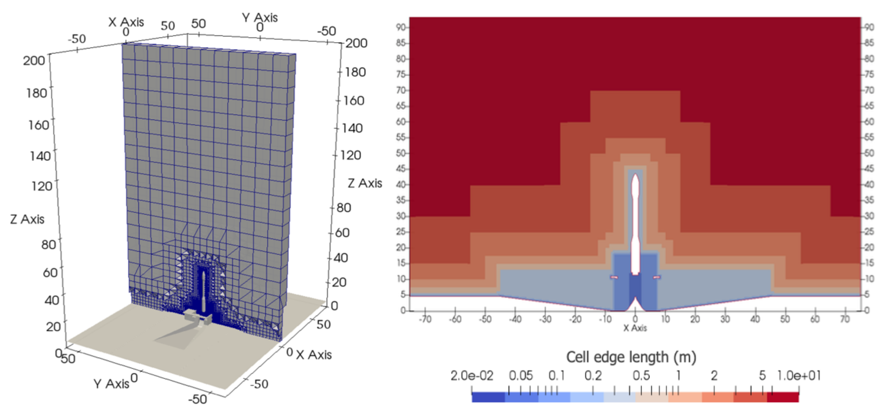
2.2. Geometry and Mesh

The geometry of the model includes the VEGA rocket, the launcher support system, the flame deflector, the exhaust ducts, and the floor. As the objective was to evaluate the noise source regions without significantly increasing the number of mesh elements, the focus was on the region where the jet plume develops and impacts the deflector. A mesh study of the jet region was performed in [16]. Finally, a mesh with 10 million hexahedral elements and a cell size of 0.078 m in the jet region was generated. The fluid domain of the study is shown in Figure 2 together with a representation of the mesh cells and their size.

2.3. Flow Conditions and Numerical Schemes

The physical properties related to the exhaust plume were calculated with the isentropic flow equations through a Laval nozzle. The supersonic inlet conditions were applied at the end of the nozzle of the VEGA rocket and were depicted in [13]. As the discontinuities that occur in supersonic flows affect the stability and accuracy of the calculation, it is crucial to choose a suitable solver and numerical schemes. The solver used was rhoPimpleCentralFoam, a transient and compressible solver developed by Kraposhin et al. [17]. More details regarding the simulation can be found in [13].

3. Results and Discussion

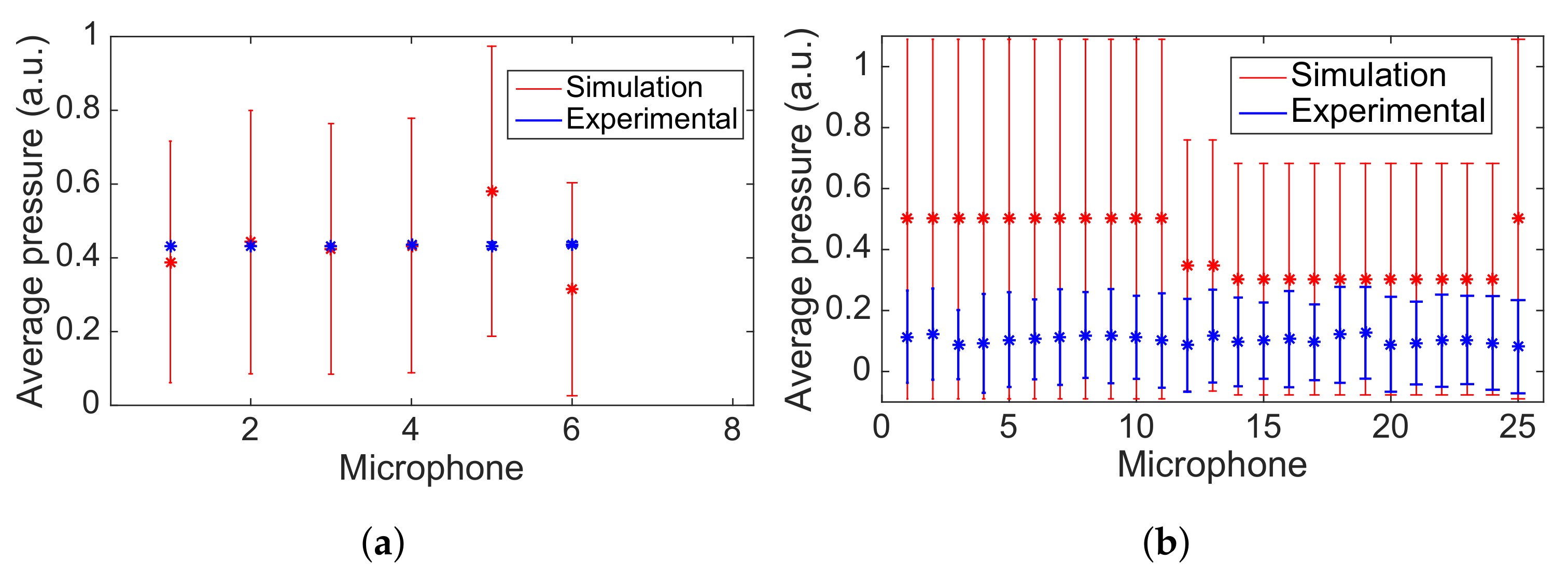
3.1. Validation of the Results

Experimental data to validate CFD models are scarce in the vicinity of the exhaust gases. Hence, two sets of acoustic data measured during the lift-off of the VEGA launch system were provided by ESA.

The first set of experimental data were extracted from a phased array of microphones located at one of the masts surrounding the launch platform, as those shown in [18]. The second set consisted of the measurements of six microphones along the fairing surface. As the experimental data are confidential, the results were normalized. Figure 3 shows a comparison of the time-averaged value of total pressure at each microphone with the equivalent positions translated to simulations. The comparison was performed in terms of the mean value of pressure and its standard error. Hence, the vertical line represents the acceptable range calculated as the mean value ± the standard error, and the marker represents the mean value. The blue results represent the experimental measures, and the red represents the simulation results. The comparison at the fairing surface in Figure 3a shows the average pressure for the six microphones. The mean pressure obtained at Microphones 2, 3, and 4 from the simulation was within the acceptable range of the experimental measurements, whereas none of the other microphones were. These microphones had less than a 3% error. Concerning the pressure along the microphone array placed at a mast, shown in Figure 3b, the mean pressure obtained by the simulation was not within the experimentally acceptable range. However, the experimentally acceptable range was within the mean minus the simulation’s standard error. In this region, the performance of the CFD model was not ideal. Factors such as the simplification of the exhaust plume input data or the movement of the rocket led to different sources of error in both locations. However, the parameters obtained at the plume development region and the flow behavior agreed with the literature [13], and the results at the fairing presented a better accuracy.

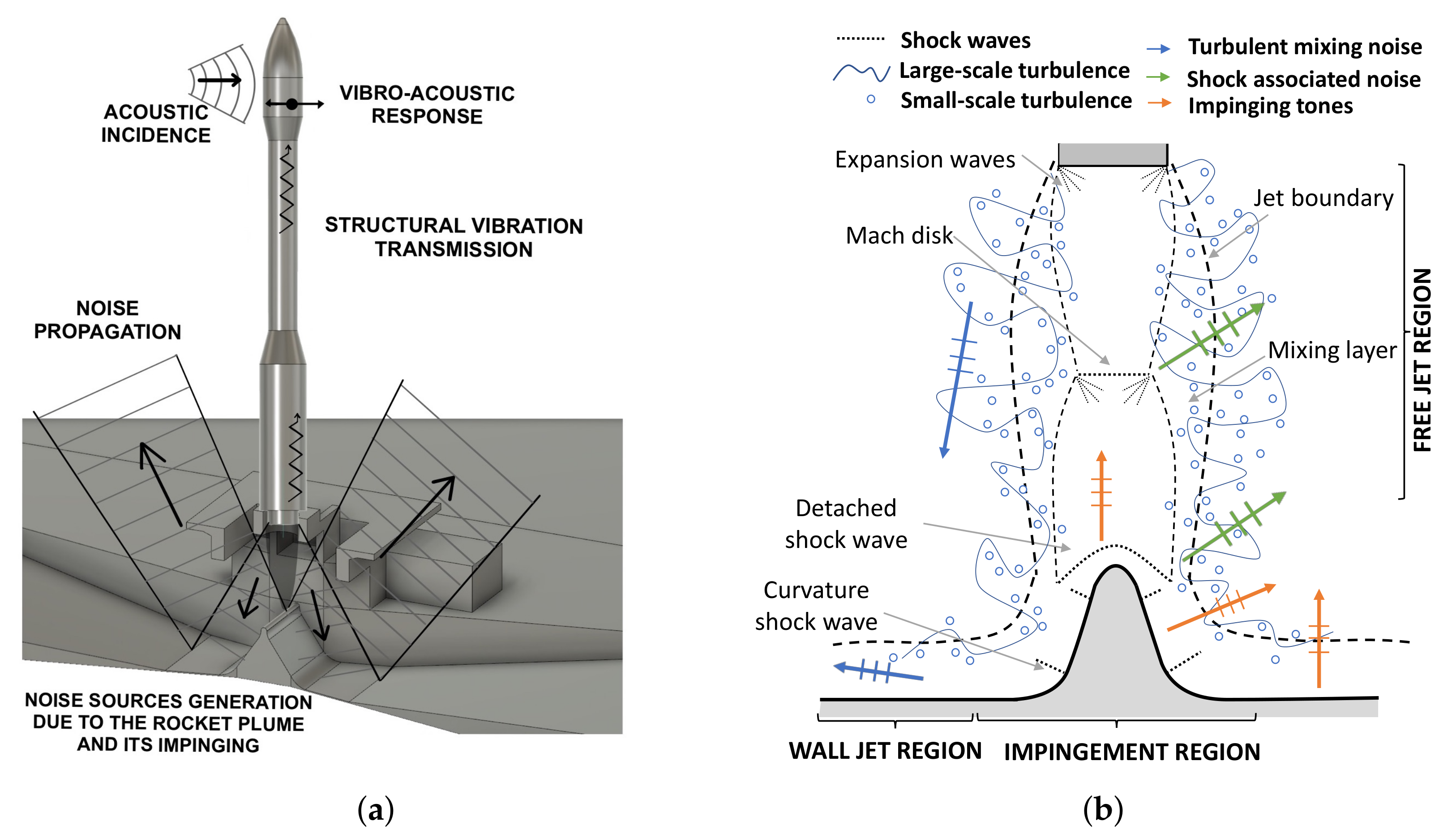
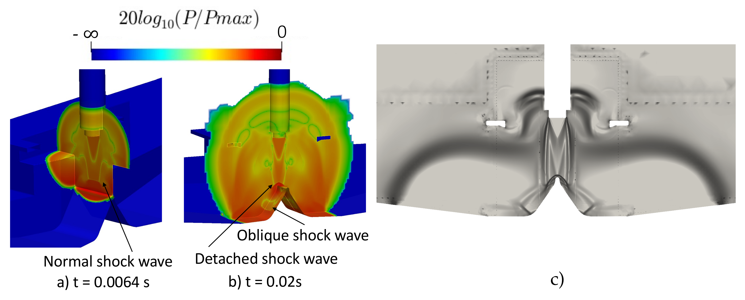
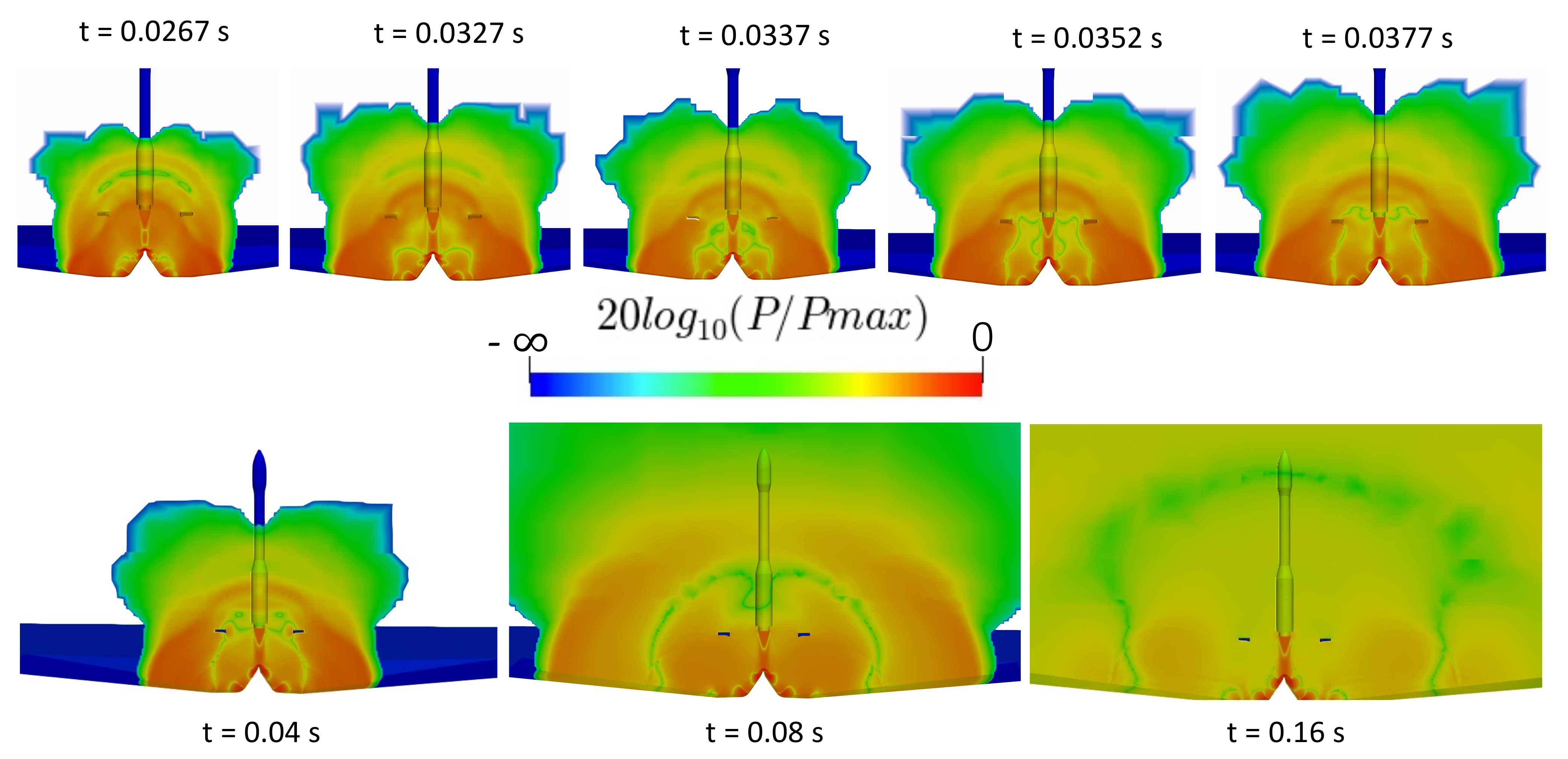
3.2. Noise Source and Propagation

The identification of noise sources started with the study of shock waves, as these are among the main noise generation phenomena during lift-off. The instantaneous pressure was represented in logarithmic scale to visualize the regions where the sound pressure was higher. Because the jet flow was supersonic, there was a normal shock wave that generated the maximum pressure value, as shown in Figure 4a. As the flow moved, the wave was deformed by the presence of the deflector, resulting in the detached shock wave, as seen in Figure 4b. At this instant, the maximum pressure levels were due to the impact of the normal shock wave with the deflector. Later, the wavefront remained at the curvature between the deflector and the floor due to an oblique shock wave. Figure 4c shows a numerically obtained version of the Schlieren images, which capture the density variations of the fluid. The main shock waves observed were those caused by the jet and the moving flow on the platform, the detached wave on the deflector, and the oblique shock wave caused by the ramp curvature change. In this way, all of these disturbances were noise-generating sources.

Figure 4b at t = 0.02 s depicts the evolution of the blast wave due to the rocket exhaust gases. There is a green wavefront that corresponded to the jet core boundary and a second one that emerged from the nozzle and moved downstream while being disrupted by launchpad elements. The evolution of this second wavefront can be seen in the top images of Figure 5, between 0.0267 s and 0.0377 s. It was caused by the initial exit of the gases and their impact on the deflector. As it moved upstream, it was disrupted by the elements of the structure. Between 0.04 s and 0.16 s, the blast wave continued to advance upstream. At the same time, the waves generated by the interaction with the support structure separated from the wave generated at the output of the jet. Due to the faster sound propagation speed, the wavefront eventually overtook the fluid front and was attenuated. At the final time step, the maximum pressure values were found in the jet development region and the deflector due to the supersonic velocity and shock waves that appeared. On this basis, it can be concluded that the maximum pressure levels were produced by the initial normal shock wave and its subsequent impact with the deflector. The acoustic waves propagated upstream of the vehicle due to this impact and the effect of the flow movement.

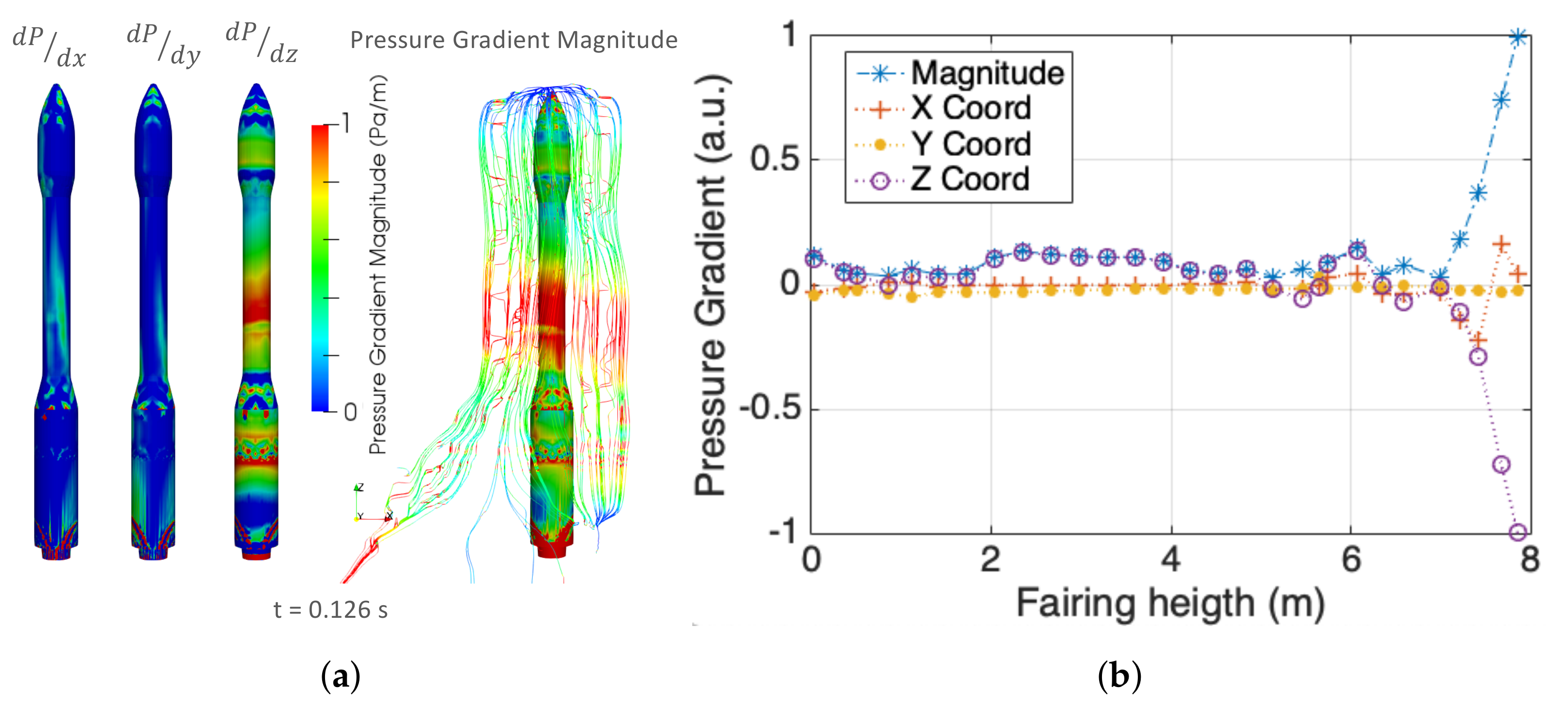
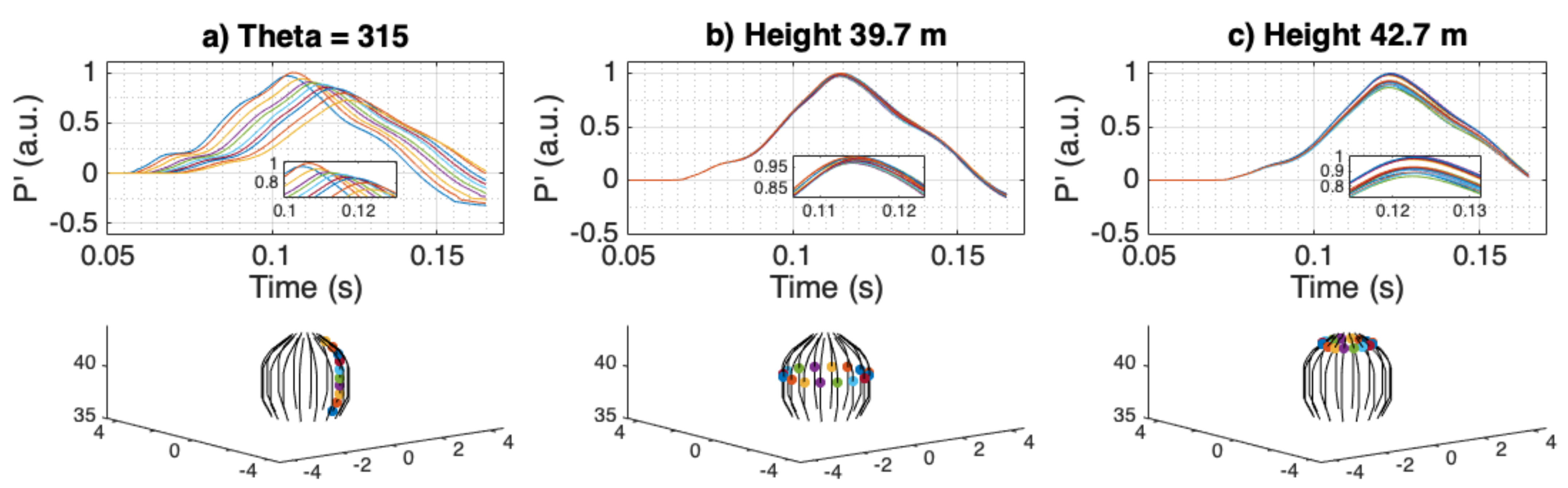
3.3. Incidence of the Pressure Field on the Fairing

To model the vibroacoustic response of the fairing, it was necessary to know how the pressure field around the fairing was. A diffuse acoustic field is usually used to model the acoustic excitation in vibroacoustic analysis [19]. Taking advantage of the CFD results, this hypothesis can be assessed. A total of 176 sampling points around the fairing were computed to evaluate the pressure field. These points were separated into 11 axial planes with 16 equispaced points.

Figure 6 shows, in (a), the results obtained for a set of points placed at different heights and, in (b) and (c), the results for two sets at the same height, but different azimuth angles. As seen in Figure 6a, the pressure increased as the exhaust gases’ wavefront moved upstream. After reaching the maximum, the pressure decreased as a result of the second wavefront seen in Figure 5. For different height planes, the gauge pressure was delayed in time. Moreover, the maximum peak pressure decreased with height because the magnitude of the pressure wave decreased as it propagated.

The discrepancy in the pressure between points at the same height was small, as seen in Figure 6b,c. However, there was an increase in this difference with the increase in height. The maximum pressure variation between points on the same plane was about 1/10 of that for the points at different heights. This was mainly because the fluid front reached each plane at a different time. It should also be noted that the region at the lower part of the fairing supported bigger pressure values than the upper region.

As the pressure gradient can be used to assess the direction of pressure waves, it was studied from the simulation results. Figure 7a depicts the pressure gradient in each direction, its magnitude, and the pressure gradient streamlines. The pressure gradient at the X and Y coordinates was lower than the axial direction. The streamlines show that the pressure gradient moved axially and converged at the tip of the payload fairing. As seen in Figure 7b, the Z negative component was the main contributor to the pressure magnitude at the tip. This negative component created a gradient pressure force that attracted the flow. This gradient decreased as the pressure wave weakened, with the maximum values occurring around t = 0.1 s. With this analysis, it is clear that the pressure field had a vertical direction due to the movement of the exhaust gases.

4. Conclusions

In the context of designing a noise-reduction system to improve sound attenuation during space vehicles’ launch, a numerical modeling framework was defined to predict acoustic loads. CFD was used to assess the noise generation and propagation mechanisms in the low-frequency regime. The reliable analysis of this type of environment involves considering many variables and physical phenomena such as the combustion of gases, the compressibility of the supersonic flow, and the lift of the launch vehicle. In addition, if we want to solve the generated turbulence and with a sufficient resolution from the acoustic point of view, the simulation of a rocket launch requires an extremely high computational and engineering cost that is out of industrial reach. In this work, the simulation was simplified to model this complex environment from the engineering point of view. The main requirements were to minimize the computational time while modeling the phenomena accurately. Thus, it was evaluated whether URANS-type modeling offered sufficient accuracy at a low computational cost.

A limitation of the work was that there were no experimental data close to the rocket engine. Therefore, data on the far-field and fairing surface were used. The validation showed a better data correlation at the fairing surface than in the masts surrounding the launch pad. The apparent lack of correlation could be attributed to different sources of error as the simplification of the launch pad structures, of the exhaust gases thermodynamics, or URANS modeling. However, there was a bigger refinement of the cells at the fairing rather than at the far-field points. Hence, this was reflected in the better prediction of the results. The primary refinement was in the region where the jet develops. Upstream, the cells’ size increased to reduce the computational cost. The approximate computational time to simulate 0.1 “real-life” s of the ${10}^6$ element mesh with 128 processors was 33 d, which is a substantial amount. Moreover, a collateral issue was the large amount of data generated for each step. The greater the mesh, the greater the amount of data was. Further work should address the effect of the mesh size in this region on the accuracy and computational cost.

The results found that the sound pressure maxima appeared due to the normal shock wave generated by the jet and its impingement with the deflector. Moreover, the shock waves present were visualized by numerical Schlieren pictures. Furthermore, the vertical directivity of the pressure over the fairing and the propagation of upstream sound waves were observed. These findings showed that the diffuse field did not represent the acoustic field that excited the fairing.

Finally, these results provided insight into the phenomena during a rocket lift-off. The knowledge regarding the noise propagation paths will help design the noise reduction systems and define their positioning on the launch pad.

References

1. Eldred, K.M. Acoustic Loads Generated by the Propulsion System; Technical Report; National Aeronautics and Space Administration: Washington, DC, USA, 1971.
2. Jiang, C.; Han, T.; Gao, Z.; Lee, C.H. A review of impinging jets during rocket launching. Prog. Aerosp. Sci. 2019, 109, 100547. [Google Scholar] [CrossRef]
3. Arenas, J.P.; Margasahayam, R.N. Noise and vibration of spacecraft structures. Ingeniare. Rev. Chil. Ing. 2006, 14, 251–264. [Google Scholar] [CrossRef]
4. Nonomura, T.; Nakano, H.; Ozawa, Y.; Terakado, D.; Yamamoto, M.; Fujii, K.; Oyama, A. Large eddy simulation of acoustic waves generated from a hot supersonic jet. Shock Waves 2019, 29, 1133–1154. [Google Scholar] [CrossRef]
5. Tam, C.K. Supersonic jet noise. Annu. Rev. Fluid Mech. 1995, 27, 17–43. [Google Scholar] [CrossRef]
6. Hoyas, S.; Oberlack, M.; Kraheberger, S.; Álcantara-Ávila, F.; Laux, J. Wall turbulence at high friction Reynolds numbers. Phys. Rev. Fluids, 2021; to appear. [Google Scholar] [CrossRef]
7. Gusman, M.; Housman, J.; Kiris, C. Best Practices for CFD simulations of launch vehicle ascent with plumes-overflow perspective. In Proceedings of the 49th AIAA Aerospace Sciences Meeting including the New Horizons Forum and Aerospace Exposition, Orlando, FL, USA, 4–7 January 2011; p. 1054. [Google Scholar]
8. McGuirk, J. Propulsive jet aerodynamics and aeroacoustics. Aeronaut. J. 2022, 126, 2–58. [Google Scholar] [CrossRef]
9. Tatsukawa, T.; Nonomura, T.; Oyama, A.; Fujii, K. Multi-objective aeroacoustic design exploration of launch-pad flame deflector using large-eddy simulation. J. Spacecr. Rocket. 2016, 53, 751–758. [Google Scholar] [CrossRef]
10. Xing, C.; Le, G.; Shen, L.; Zhao, C.; Zheng, H. Numerical investigations on acoustic environment of multi-nozzle launch vehicle at lift-off. Aerosp. Sci. Technol. 2020, 106, 106140. [Google Scholar] [CrossRef]
11. Chin, C.; Li, M.; Harkin, C.; Rochwerger, T.; Chan, L.; Ooi, A.; Risborg, A.; Soria, J. Investigation of the Flow Structures in Supersonic Free and Impinging Jet Flows. J. Fluids Eng. 2013, 135, 031202. [Google Scholar] [CrossRef]
12. Camussi, R.; Di Marco, A.; Stoica, C.; Bernardini, M.; Stella, F.; De Gregorio, F.; Paglia, F.; Romano, L.; Barbagallo, D. Wind tunnel measurements of the surface pressure fluctuations on the new VEGA-C space launcher. Aerosp. Sci. Technol. 2020, 99, 105772. [Google Scholar] [CrossRef]
13. Escarti-Guillem, M.S.; Hoyas, S.; García-Raffi, L.M. Rocket plume URANS simulation using OpenFOAM. Results Eng. 2019, 4, 100056. [Google Scholar] [CrossRef]
14. Wilcox, D.C. Turbulence Modeling for CFD; DCW Industries: La Cañada, CA, USA, 1998; Volume 2. [Google Scholar]
15. Menter, F. Zonal two equation kw turbulence models for aerodynamic flows. In Proceedings of the 23rd Fluid Dynamics, Plasmadynamics, and Lasers Conference, Orlando, FL, USA, 6–9 July 1993; p. 2906. [Google Scholar]
16. Ramírez, F.N.; Escarti-Guillem, M.S.; García-Raffi, L.M.; Hoyas, S. A study of the mesh effect on a rocket plume simulation. Results Eng. 2022, 13, 100366. [Google Scholar] [CrossRef]
17. Kraposhin, M.V.; Banholzer, M.; Pfitzner, M.; Marchevsky, I.K. A hybrid pressure-based solver for nonideal single-phase fluid flows at all speeds. Int. J. Numer. Methods Fluids 2018, 88, 79–99. [Google Scholar] [CrossRef]
18. Mortain, F.; Cléro, F.; Palmieri, D. Full Scale Acoustic Source Identification on VEGA Launch Pad at Lift-Off. In Proceedings of the ICSV26, Montreal, QC, Canada, 7–11 July 2019. [Google Scholar]
19. Secretariat, E. Spacecraft mechanical loads analysis handbook. In European Cooperation for Space Standardization; ESA Requirements and Standards Division: Noordwijk, The Netherlands, 2013. [Google Scholar]
Figure 1. Sound generation and transmission during a rocket launch. (a) Scheme of noise transmission paths. (b) Scheme of noise sources due to the rocket plume.
Applsci 12 03356 g001
Figure 2. Mesh details. On the left picture, mesh domain cross-section representing each of the cells. On the right, representation of the mesh classified by the size of the cells.
Applsci 12 03356 g002
Figure 3. Time-averaged pressure validation against experimental measurements along (a) the VEGA fairing and (b) one of the masts. Results are normalized.
Applsci 12 03356 g003
Figure 4. VEGA lift-off environment shock waves’ identification. Normalized instantaneous pressure contour at (a) t = 0.0064 s and (b) t = 0.02 s. (c) Schlieren shock waves’ identification.
Applsci 12 03356 g004
Figure 5. Normalized instantaneous pressure contour of VEGA launch pad environment.
Applsci 12 03356 g005
Figure 6. Pressure temporal evolution along the fairing at (a) an azimuth angle of 315° and different heights, (b) at a constant height of 39.7 m with different azimuth angles, and (c) at 42.7 m and different azimuth angles.
Applsci 12 03356 g006
Figure 7. Pressure gradient magnitude and components. (a) Graphical representation at t = 0.126 s. (b) Plot over the fairing axial plane.
Applsci 12 03356 g007
Publisher’s Note: MDPI stays neutral with regard to jurisdictional claims in published maps and institutional affiliations.