Abstract
Due to poor predictability of resources and difficulty in perception of task execution status, traditional Automatic Guide Vehicle (AGV) scheduling systems need a lot of extra time in the charging process. To solve this problem, a digital twin-based dynamic AGV scheduling (DTDAS) method is proposed, including four functions, namely the knowledge support system, the scheduling model, the scheduling optimization, and the scheduling simulation. With the features of virtual reality data interaction, symbiosis, and fusion from the digital twin technology, the proposed DTDAS method can solve the AGV charging problem in the AGV scheduling system, effectively improving the operating efficiency of the workshop. An AGV scheduling process in a discrete manufacturing workshop is taken as a case study to verify the effectiveness of the proposed method. The results show that, compared with the traditional AGV scheduling method, the DTDAS method proposed in this article can reduce makespan 10.7% and reduce energy consumption by 1.32%.
1. Introduction
AGV scheduling is a crucial process in manufacturing systems [1,2]. It aims at the allocation and timing management of transportation tasks to achieve goals such as reduction in completion time, energy consumption, and resource idle rate [3,4]. In recent years, AGV scheduling optimization has been continuously improved with the development of advanced methods, such as the math programming method [5], the agent-based method [6], the machine learning method [7], etc. Although these novel methods have been involved in the scheduling, the accurate description of AGV property, such as the charging process, is always ignored. However, charging process of the AGV may take several hours, which may result in serious interruption and delay of the transport tasks. So, charging behavior should be carefully considered, otherwise, the scheduling cannot be well optimized.
AGVs are normally powered by the batteries. In the actual shop flow, the AGV will break the task when the state of charge (SOC) of the battery reaches a certain threshold [8,9]. Consequently, the AGV should be charged autonomously in the nearest charging area. However, this charging mode for AGVs may be harmful to the overall performance of the system [10]. When the battery power of the an AGV drops below the threshold, the current position of the AGV can, by chance, be far away from the charging area. Charging in advance at charging area closer to the initial position could be a better decision. This would decrease the total extra travel time from the work area to the charging area. Furthermore, the AGVs are normally fully charged with long charging time. Charging a portion of the AGV may be more reasonable when a rush transportation task is needed.
Therefore, in addition to a module for allocating transport tasks, a battery management module for allocating charging tasks should also be included for a complete AGV scheduling system [11,12]. Research in the field of AGV scheduling has begun to pay attention to battery management in recent years. Kabir et al. [13] explored the production capacity of the workshop through battery management. The results showed that more frequent charging of AGVs increases the productivity of the manufacturing system significantly. Ryck et al. [10] proposed an AGV scheduling method based on the TSP (Traveling Salesman Problem) model, which acquires the optimal charging timing and time to reduce the task completion time. These studies can reduce the impact of the charging process on the execution of AGV tasks with static scheduling methods. However, scheduling systems using the static method has limited performance in a real production environment, since the status of a real production environment is changeable.
In order to improve the adaptability of the scheduling system to the environment, dynamic scheduling methods are studied. Heger et al. [4] proposed a scheduling method based on dynamic priority, which becomes the commonly used AGV dynamic scheduling method. Sahin et al. [6] proposed an agent-based dynamic scheduling method. Each agent in the system was autonomous and could negotiate and cooperate with other agents. Smolic-Rocak et al. [14] proposed a dynamic planning method for AGV based on the time window. However, these research works have some common shortcomings. Firstly, with a predefined mathematical model, these solutions cannot possibly describe the status of the AGV accurately and dynamically. Secondly, these methods cannot predict the AGV’s availability for a period of time, so a global optimal scheduling plan cannot be obtained. Hence, for the AGV scheduling considering battery management, there are still many limitations if the traditional dynamic scheduling methods are used.
Digital twin has been widely used in manufacturing in recent years [15,16], providing a new solution to the scheduling problem of the workshop. Liu et al. [17] believe that with the characteristics of virtual reality data interaction and fusion, digital twin technology can improve shop-floor performance in the scheduling decision-making process. Fang et al. [18] proposed a digital twin-based job shop scheduling method. Compared to traditional scheduling methods, it can obtain more accurate data for rescheduling and timely response to dynamic events. Zhang et al. [19] proposed a DT-enhanced dynamic scheduling method for machine task assignment. The results show that this method can reduce manufacturing time and delays. In general, the application of digital twin in manufacturing brings a chance to promote scheduling technology. On the one hand, by establishing a digital twin workshop, the working status and task progress of the physical workshop can be mapped to the virtual workshop to track and improve the production process [20]. On the other hand, the digital twin system collects a large amount of data from physical workshops and virtual workshops, which provides sufficient data support for workshop production [21]. Hence, the digital twin based dynamic scheduling system can meet the needs of real-time scheduling and strong predictability.
To utilize the advantage of the digital twin technology and solve the problems mentioned above, a digital twin-based dynamic AGV scheduling (DTDAS) method is proposed in this paper. A dynamic energy consumption model is first established to describe the latest energy consumption characteristics of AGV. The prediction method for AGV availability based on the current scheduling plan and dynamic energy consumption models is then proposed. Thirdly, a digital twin-based AGV scheduling system is constructed. The main contribution of this paper includes: (1) A proposal for an overall framework of digital twin-based dynamic AGV scheduling; (2) Exploration of the methods for building an AGV dynamic energy consumption model, and digital twin-based AGV availability prediction; (3) The building of a mathematical model of initial scheduling and charging scheduling. The proposed methods are validated by taking a batch of orders in the discrete workshop as a case study.
2. Problem Formulations
This paper considers the AGV scheduling in in a discrete manufacturing workshop producing parts for internal combustion engines, as shown in Figure 1. The workshop includes six machines for processing parts and three AGVs for transporting parts.
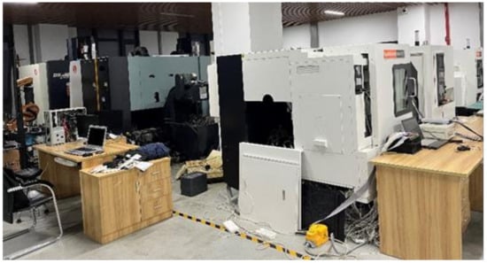
Figure 1.
Discrete manufacturing workshop.
The general layout of the workshop is shown in Figure 2. Here, only the AGV scheduling is considered, and the allocation of the machine has been completed by default. Therefore, each workpiece process in the processing corresponds to a unique machine. In the material storage area S, the blanks of the workpieces are initially placed. The blanks are carried by the AGV to the corresponding machine Mx after an order is placed. After several processes, the finished workpieces are transported by AGV to the parts storage area F. A simple example is shown in Figure 1. Order 1 contains two machining operations, which will be performed on M2 and M6, respectively. Consequently, three transport tasks with time-constrained are generated, Task 1 (S–M2), Task 2 (M2–M6) and Task 1 (M6–F). These three transportation tasks will be performed by AGV1, AGV2 and AGV3, respectively. The AGV will charge in the case of insufficient power before the performance of transportation tasks.
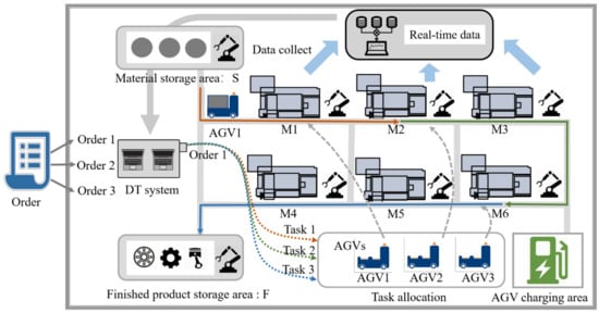
Figure 2.
The layout of the manufacturing workshop.
The studied dynamic scheduling problem is subjected to the following assumptions:
- AGV’s collision and deadlock are not considered;
- The AGV drives with the principle of the shortest path;
- An AGV can only carry one workpiece each time;
- AGV loading and unloading time can be ignored;
- Charging devices are capable for all AGVs at the same time;
- AGV cannot perform charging tasks during transportation;
- There is no capacity limit for material storage areas and finished product storage areas;
- The speed of the AGV remains constant during driving.
3. Principle of the Proposed DTDAS
The framework of DTDAS consists of two parts: the physical workshop and the virtual workshop. As shown in Figure 3, the two parts share data. The real-time data in the physical workshop are transmitted to the scheduling model in the virtual space. The scheduling plan generated by the virtual workshop is then sent to the physical workshop. There are four modules in the virtual space: the knowledge support module, the scheduling model module, the scheduling optimization module, and the simulation verification module. In the knowledge support module, the dynamic energy consumption model and the AGV availability prediction provide a decision basis for the scheduling model. The scheduling model includes the allocation of transportation tasks and the allocation of charging tasks. This scheduling model will be solved by the scheduling optimization algorithm. After the simulation verification, the obtained scheduling plan is sent to the execution system, assigning tasks further to the corresponding equipment.
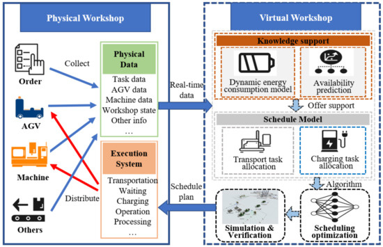
Figure 3.
The framework of DTDAS.
3.1. Knowledge Support
3.1.1. AGV Dynamic Energy Consumption Model
In this article, only the unavailable state caused by insufficient power of the AGV is considered. Other reasons, such as AGV failure, are neglected. Accurate energy consumption calculation is the prerequisite for predicting the availability of the AGV in actual transportation. Therefore, a mathematical model is needed to accurately describe the energy consumption characteristics of AGVs. The traditional scheduling mechanism is also possible to establish an AGV energy consumption model with fixed parameter values. However, the battery used in the AGV system will show different energy consumption characteristics in different states [22]. It is difficult to accurately describe the energy consumption characteristics when the workshop status changes. Digital twin connected with abundant real-time data resources provides data support for the establishment of dynamic energy consumption models. This paper adopts the method of real-time data fitting, as shown in Figure 4. AGV speed, load, and battery state of charge (SOC) are taken as input. AGV’s energy consumption rate is taken as the output to establish the AGV’s energy consumption model to describe the AGV’s energy consumption characteristics at different loads and speeds. It should be noted that the SOC of the AGV battery is an estimated value obtained by current and voltage [23], which is regarded as a given value in this paper to simplify the dynamic energy consumption model. Hence, the dynamic energy consumption model can be expressed as:
where is the estimated energy consumption rate of transport task i, mass and represent AGV load and speed, respectively, , are the correlation coefficients, is offset value. And is real-time energy consumption rate, is the estimated error of the energy consumption rate. The symbols appearing in this paper can refer to the Appendix A.
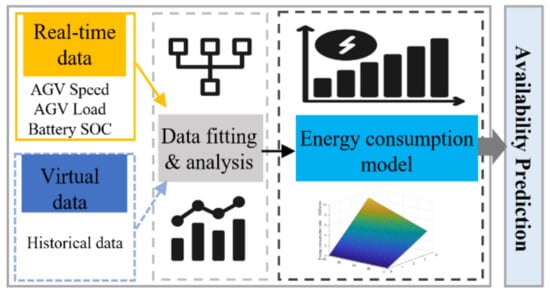
Figure 4.
Real-time data based AGV energy consumption model.
When is under a certain threshold, this estimation formula is maintained. When is greater than this threshold, this formula will be replaced by the formula fitted from the latest data. This data model will provide support for the AGV availability prediction.
3.1.2. AGV Availability Prediction
During the operation of the workshop transportation system, AGV failures, AGV low battery warnings, etc., are the main reasons for delaying the production plan. The DT-based dynamic scheduling system should avoid such events from origin through prediction and status monitoring. Since the AGV failure period usually only accounts for a small part of the working cycle, this article mainly discusses the impact of the charging process on availability. The previous section describes the establishment of the AGV energy consumption model in the digital twin system. As shown in Figure 5, the model can be based on the current SOC and schedule plan to predict the electricity characteristics of AGV operation for a while in the future. Generally, AGV battery SOC dropping to 20% is considered unavailable. Then we can obtain the AGV’s availability result based on the predicted value of the AGV battery SOC, which will be used as the basis for the scheduling system to perform the charging schedule. The predicted value of the AGV battery SOC can be expressed as:
where
is the predicted value of AGV battery SOC at time t, is the initial value of AGV battery SOC. is the time required to perform transport task i.
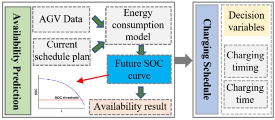
Figure 5.
AGV Availability Prediction.
3.2. Scheduling Model
The scheduling model built in this article is divided into two parts: the initial scheduling part and the charging scheduling part. The initial scheduling contains two decision variables: the allocation of transportation tasks and the timing management of the transportation tasks. The charging schedule also contains two decision variables: the allocation of AGV charging tasks and the allocation of charging capacity.
The allocation of transportation tasks can be expressed as:
The management of task execution timing can be expressed as:
when , ; when , .
The allocation of charging tasks can be expressed as:
The decision on charging power can be expressed as:
In the initial scheduling process, reducing the makespan and the energy consumption of the AGV system is the goal. To ensure that the transportation tasks are completed as early as possible during the charging schedule without affecting the production process, we hope to arrange the charging tasks for the AGV as much as possible during the idle period of the initial scheduling plan. At the same time, the charging frequency should not be too much (It is impossible to schedule AGV charging for all idle periods), which will cause a lot of unnecessary energy consumption. As a result, we consider makespan and energy consumption as the optimization goal of the charging schedule. In fact, it is also possible to insert the charging task during the initial scheduling process, however the model of this method is more complicated, and its calculation time is unacceptable for the dynamic scheduling system.
Minimizing the makespan. Makespan means the maximum completion time, which can be expressed by:
Subject to
where Equation (10) calculates the start time of the transportation process according to whether the charging process is included before task execution. Equation (11) calculates the time taken by the AGV to perform the charging task, including the time for the AGV to go to the charging area and the time to charge in the charging area. The waiting time for the AGV to perform this transportation task is determined by Equation (12). Equations (13) and (14) ensure that the time sequence of the transportation task meets the requirements. Equation (15) ensures that from the second transportation operation of each order, the start time of the transportation task must be greater than the processing completion time of the machine. Equation (16) ensures that each transportation task will only be executed once. Equation (17) ensures that the start time of this processing operation must be greater than the end time of the previous transportation operation. Among them, the first transportation operation is transported from the material storage area to the corresponding machine, so there is no corresponding processing operation.
Minimizing the total energy consumption. Energy consumption is expressed by AGV battery SOC. The total energy consumption can be expressed by:
Subject to:
Equation (19) is the AGV real-time power soft constraint, which ensures that the AGV will not perform transportation tasks when the power is less than 20%. Where, is a small positive number. Equation (20) ensures that the AGV battery will not be overcharged due to each charging process. Equation (21) calculates the total power charged to Aa when completing all transportation tasks. Equation (22) calculates the total electricity consumed by Aa in the transportation operation. Equation (23) calculates the final power of Aa when all transportation tasks are completed. The energy consumption rate of AGV during transport is determined in Equation (24) for different transport operation loads.
Multi-objective evaluation. The objective function consists of two components: makespan and energy consumption, which can be expressed as:
where is the weight coefficient of MS, and is a coefficient to adjust the two objectives in the same order of magnitude.
3.3. Scheduling Optimization
A Genetic algorithm (GA) is one of the most popular multi-objective optimization algorithms. It has the characteristics of a good optimization effect and fast convergence speed, which is an effective method to solve this kind of scheduling problem. Therefore, this paper uses GA to solve the mathematics model mentioned above.
3.3.1. Solution of the Coding
The first section is the coding of the problem’s solution. This article divides the chromosome into four segments, corresponding to the four decision variables in the model mentioned above. As shown in Figure 6, assuming that there are four orders in the scheduling that contain a total of 17 transportation operations, the entire chromosome contains 68 genes, and each gene fragment contains 17 genes. The first part reflects the transportation operation’s priority, decreasing from left to right, and the gene’s code defines transportation operations related to for each order. The genetic code is the same as their order number, so that all the genes related to operations have the code “1” and subsequently the code “2” is given to all the genes related to , and so on. So the first “1” represents and the first “2” represents . The second segment of the genetic code is the AGV number, and this genetic code defines which AGV will transport the corresponding transportation operations. The third segment represents the allocation of charging tasks, which are all Boolean variables. The last segment of the genetic code represents the amount of charge when the AGV is charging. For example, genetic number two corresponds to the transportation operation , which will be carried by the AGV numbered two. The AGV numbered two will go to the charging area to charge once before the transportation, and the charged power is 20.
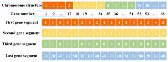
Figure 6.
A randomly generated chromosome and the gene segment.
3.3.2. Algorithm Configuration
Fitness function. The fitness function in this paper can be expressed as:
Selection. This article adopts a roulette method for individual selection to constantly increase the overall fitness of the population.
Crossover. The corresponding gene exchange between different individuals can result in illegal individuals when the chromosomes cross. At this time, the individual needs to be repaired reasonably, and the repair method can be referred to [24].
Mutation. This paper introduces shift mutation on the first gene segment of the chromosome to ensure that a legal individual is produced during the mutation process. The particular methods are presented in [25], and general methods of mutation are used for other segments.
Elitism. The best individuals will be directly transferred to the next generation of populations in the elite process.
In the initial scheduling, only the first and second segments of the chromosome are operated. In the charging scheduling, only the third and fourth segments of the chromosome are operated.
3.4. Simulation Verification
As shown in Figure 7, this module includes two parts, visualization simulation and evaluation simulation. Visualization of the scheduling process is the basic function of this module. Firstly, we build the 3D model of the AGVs and import them into Flexsim (A 3D Simulation Modeling and Analysis Software), as shown in Figure 8. Then, the process flow and data interface of the AGV are established. The Emulation module in Flexsim is used to establish the Modbus TCP Connection, as shown in Figure 9. Finally, the acquired sensor data of the physical device is transmitted to Flexsim through the network port. Consequently, AGVs and other devices perform pre-defined actions based on these real-time data.
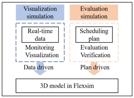
Figure 7.
Simulation and Verification.
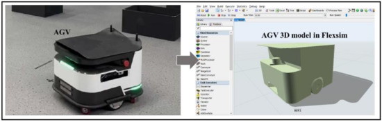
Figure 8.
AGV 3D model imported into Flexsim.
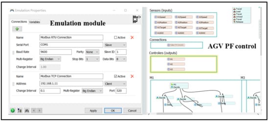
Figure 9.
Emulation module and process flow configuration in Flexsim.
Evaluation simulation refers to the simulation of the entire process before the scheduling plan is executed on the physical workshop. The 3D models in Flexsim can also be driven by scheduling plan tables. When a schedule plan is generated, it will first be sent to Flexsim for evaluation. In this way, we can dynamically evaluate the utilization rate of each AGV, the delivery and completion time, the delay time of each workpiece, etc. At the same time, the path conflict problem of the AGV system can also be found in the simulation. The evaluation indicators have a strong guiding significance for the execution system of the physical workshop. Simulation based on digital twins can evaluate the performance of the workshop from different scales according to the needs of users. In addition, since the model in the virtual workshop can be continuously updated based on real-time data, the simulation results can be closer to the real situation.
3.5. Dynamic Interaction Process
The overall interaction process of the proposed DTDAS is shown in Figure 10.
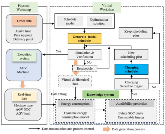
Figure 10.
The interaction process of DTDAS.
3.5.1. Generation of Initial Scheduling Plan
When an order arrives, its detailed information is transmitted to the scheduling layer. The scheduling layer, including the scheduling model and the corresponding optimization solution, generates an initial scheduling plan based on the established scheduling goals. This scheduling plan passes through the virtual system after the simulation and verification. If the simulation results show that the scheduling plan is unqualified, rescheduling will be triggered.
3.5.2. Energy Consumption and Availability Prediction
A lot of real-time data will be generated when the workshop execution system starts running. The knowledge system in the virtual space will analyze real-time data and historical data to establish a dynamic energy consumption model that can accurately describe the characteristics of AGV energy consumption. This model will be used to predict the battery SOC of the AGVs according to the latest scheduling plan and current AGV data. Therefore, the AGV’s availability can be obtained by executing the current scheduling plan continuously. If the availability results show that the power of some AGVs according to the current scheduling plan is not enough to complete the transportation tasks, the charging scheduling should be triggered. Otherwise, the original scheduling plan will be maintained.
3.5.3. Charging Scheduling
In order to change the original scheduling plan as little as possible, we keep the scheduling goal of this process consistent with it from the initial schedule. In this process, we will determine the timing and time of the AGV to perform the charging task. After the charging scheduling result is generated, it will be embedded in the initial scheduling plan and then simulated and verified. The obtained scheduling result including the charging task is transmitted to the execution system of the workshop.
When the scheduling plan is executed in the workshop, the data generated by various resources will be continuously monitored by the virtual system. The AGV availability prediction module in the virtual system and the energy consumption model can ensure that the scheduling system generates a reasonable charging scheduling plan and guarantees the generated scheduling plan including the charging process that can better approximate the actual status.
4. Case Study
4.1. Problem Description
In order to verify the effectiveness of the proposed DTDAS, a case experiment in a discrete manufacturing workshop was conducted. The layout of the workshop is shown in Figure 2 in Section 2. Figure 11 shows the location of the physical resources of the workshop with the coordinates of the points. It is assumed in the figure that the AGV’s initial location is in the charging area. The workshop order data involved in the experiment is shown in Appendix B. The task of this experiment consists of eight orders, 3~4 transportation operations in each order, and 29 transportation tasks in total. This batch of orders must be completed within 25 min. When the number of order transportation is , the number of processes is , and the first transportation operation of each order does not have a corresponding processing operation. The detail of transportation task is also in Appendix B. It contains the loading point and delivery point of each transportation task, the quality information of the transportation task, and the processing time of the processing operation corresponding to the transportation operation. The battery initial SOC of the three AGVs is shown in Table 1. Taking into account the discharge characteristics and life characteristics of the AGV battery [8], the system limits the AGV to stop performing new tasks to charge in the charging area when the AGV battery is below 20%.
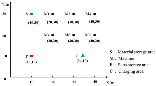
Figure 11.
Coordinates of each position in the workshop.

Table 1.
Initial battery SOC of AGV system.
The population number of the genetic algorithm is set to 100, the number of iterations is set to 200. When solving the fitness function, the value of is 0.64, is 10. The relevant parameters of AGV all come from the fitting and analysis of real-time data, is in the range of 0.27–0.45, is in the range of 0.25–0.3, is approximately 0.139. The other parameters are constant values, is 0.5 m/s, is 5, is 0.7, is 0.139.
4.2. Results and Discussion
Figure 12 shows the initial scheduling plan generated by the scheduling system based on the order data, without considering the future availability of the AGV. In the initial scheduling plan, 29 transportation tasks were completed by three AGVs in 1448 s, which met the demand that the execution system must complete all tasks within 25 min according to the order information. Figure 13 shows the AGV power curve predicted in the virtual model when the task is executed according to the initial schedule.
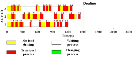
Figure 12.
Initial scheduling plan.
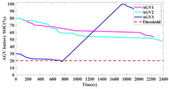
Figure 13.
The predicted AGV SOC curve when the initial schedule is executed.
It can be seen that the battery SOC of AGV3 will reach the charging threshold when the system time is close to 600 s. The AGV3 will perform the current transportation task and then go to charge. The charging process continues until the SOC reaches 100%. Figure 14 shows the evaluation results of the initial scheduling plan in Flexsim.
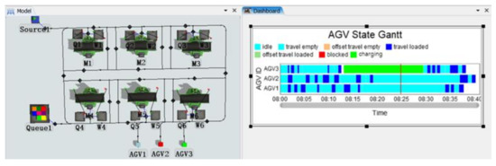
Figure 14.
Evaluation results of the initial scheduling plan in Flexsim.
The evaluation results show that makespan is 2385 s when the initial scheduling plan is executed in Flexsim. Due to the charging behaviour of AGV3, the delivery time of the task is seriously delayed and cannot be meeting the delivery requirements of this batch of orders. Furthermore, it caused a serious reduction in the utilization rate of the AGVs. Therefore, the initial scheduling plan must be adjusted.
Figure 15 shows the AGV Gantt chart under different strategies. Table 2 shows the total energy consumption of the system under different scheduling strategies. Therefore, the initial scheduling plan must be adjusted. For the scenarios described above, if the traditional dynamic scheduling method is adopted, the remaining tasks are usually redistributed when the battery of the AGV3 battery is warned. The traditional scheduling system will let the AGV3 charge immediately after the current transportation task is executed. The remaining tasks will be allocated to the other two AGVs, and the scheduling results obtained are shown in Figure 15a.
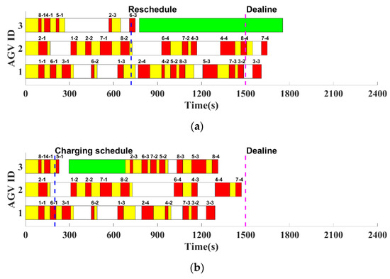
Figure 15.
AGV Gantt chart under different strategies. (a) when traditional dynamic scheduling is adopted. (b) when DTDAS is adopted.
Table 2.
Total energy consumption under different scheduling plans.
As shown in Figure 15a, the traditional dynamic scheduling can respond quickly to dynamic events. It will update the scheduling plan in time when the battery of the AGV3 is insufficient and needs to be charged, which can effectively reduce the delayed time caused by a certain AGV charging. However, the scheduling makespan generated by the traditional dynamic scheduling system is 1648 s, which still cannot meet the delivery demand.
That being said, the DTDAS proposed in this paper can predict the availability of AGV. Therefore, we can use this technology to solve the problems encountered in traditional dynamic scheduling. After the initial scheduling is generated and verified, it is sent to the execution system. The execution system starts to perform tasks and continuously feeds back data to the virtual system. At the same time, the virtual system will predict the availability of the AGV in the future. After that, it will decide whether to update the scheduling plan based on the predicted results. During the execution of the initial scheduling plan, the virtual system predicts the availability result of AGV3, and this prediction result shows that the transportation system will seriously exceed the delivery time to complete this batch of tasks. Therefore, the virtual system triggers the charging schedule in advance. In the charging schedule, the AGV3 is asked to perform a short charging behaviour before performing task 2–3. After that, AGV3 will continue to perform the transportation task. The makespan using the DTDAS proposed in this paper is 1472 s, reduced by 10.7% compared with traditional dynamic scheduling. Additionally, the total energy consumption is reduced by 1.32%.
In addition, as shown in Figure 15b, the charging process of AGV 3 is inserted before the transportation task 2–3. Compared with the initial scheduling plan, the charging task triggered by the DTDAS just used the idle period of AGV 3, and the charging time is relatively short. The AGV does not have to wait until the battery is fully charged, and the power of this charging process will be determined according to the follow-up task arrangement of this AGV. It can be seen from Figure 16 that the amount of charge can just meet the needs of completing the transportation task of this batch of orders. In this way, not only can the task completion time be shortened, but it also has the effect of effectively using power resources. The scheduling plan including the charging schedule has almost no impact on the distribution of transportation tasks. The time to complete the task is almost the same as the initial scheduling. Compared with the traditional dynamic scheduling method, the DTDAS proposed in this paper can not only shorten the makespan and reduce energy consumption, but also save a lot of rescheduling computing resources.
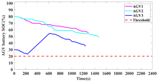
Figure 16.
The AGV SOC curve when DTDAS is adopted.
5. Conclusions
A digital twin-based dynamic AGV scheduling (DTDAS) method has been proposed in this paper. An overall framework of DTDAS was presented first. Then the knowledge support system of DTDAS was explored. A new mathematical model of AGV scheduling was finally established. Compared to the traditional dynamic scheduling method, the proposed DTDAS can not only obtain more accurate data to support the scheduling model, but also evaluate and visualize the AGV scheduling process. Meanwhile, the battery management was integrated into the mathematical model of AGV scheduling. Hence, the presented DTDAS can reasonably arrange the charging process to effectively improve the operating efficiency of the AGV transportation system in a workshop. A case study has been carried out and compared the traditional dynamic scheduling method, and it was found that the proposed method can reduce makespan and energy consumption by 10.7% and 1.32%, respectively. In general, this paper provides a new solution to the AGV scheduling problem in discrete manufacturing workshops. The application of digital twin mainly enhances the AGV scheduling technology in two aspects, providing knowledge support before the scheduling plan is generated, and comprehensive evaluation after the scheduling plan is generated. The great potential of DTDAS has been demonstrated by considering the charging problem of AGV in a manufacturing workshop. The DTDAS can theoretically be extended to any workshop with rechargeable AGVs to improve the efficiency of the transport system. However, the dynamic events considered in this paper are not comprehensive enough. In future work, the impact of other dynamic events like AGV failures or emergency tasks that occur on the scheduling system and their corresponding scheduling strategies will be studied.
Author Contributions
Conceptualization, J.X.; methodology, J.X.; software, W.H.; validation, W.H., Z.S., B.L., K.Z. and Z.Z.; formal analysis, W.H.; investigation, J.X.; resources, Z.S., K.Z. and Z.Z.; data curation, W.H., Z.S., B.L. and Z.Z.; writing—original draft preparation, W.H.; writing—review and editing, J.X. and Z.S.; visualization, Z.S., B.L. and K.Z.; supervision, J.X. and X.M.; project administration, X.M.; funding acquisition, J.X. and X.M. All authors have read and agreed to the published version of the manuscript.
Funding
This research was funded by the National Key Research and Development Program of China (2020YFB1708400).
Institutional Review Board Statement
Not applicable.
Informed Consent Statement
Not applicable.
Data Availability Statement
Not applicable.
Acknowledgments
This work was supported by the National Key Research and Development Program of China (2020YFB1708400).
Conflicts of Interest
The authors declare no conflict of interest.
Appendix A. Notation
| Nomenclature | |||
| Makespan | The time when began to be transported | ||
| The total energy consumed by all AGVs | The distance from the loading point of to the unloading point of | ||
| Order i | The time required arrive at the unloading point of from the loading point of | ||
| Index of orders, i = 1, 2, 3, … | The waiting time of at the loading point of | ||
| Total number of orders | The time when the processing operation corresponding to the transportation task began to be processed | ||
| Total number of transportation operations for each order | The time required for the processing operation corresponding to the transportation task | ||
| Transportation task j of order i | The SOC of at the initial moment | ||
| AGV numbered a | The real-time SOC of | ||
| Index of AGVs, a = 1, 2, 3, … | The SOC of at the final moment | ||
| Machine numbered x | The charging amount of after completing all task | ||
| Index of machines, x = 1, 2, 3, … | The power consumed by in completing task | ||
| AGV recharge area | will perform charging operation before performing | ||
| Material storage area | The charging amount of in the charging operation | ||
| Finished product storage areas | The time required for perform charging operation (Including driving time and charging time) | ||
| The loading point of | The time required for to arrive at AGV recharge area from the current position of | ||
| The unloading point of | The distance from the current position of to AGV recharge area | ||
| Aa is allocated to | The time required for charging in the charging operation | ||
| The start running time of the system | The distance from the AGV recharge area to the loading point of | ||
| The current position of | The time required arrive at the loading point of from AGV recharge area | ||
| The time when in the current position | Charging rate of AGV | ||
| The distance from the current position of to loading point of | Energy consumption rate coefficient under different operations | ||
| The time required from the current position of to loading point of | Part quality under different operations; | ||
Appendix B. Workshop Order Data
| Order | Transportation Operations | Loading Point | Unloading Point | Mass/kg | Processing Time/min |
| 1 | 1 | S | M2 | 10 | S:0 |
| 1 | 2 | M2 | M4 | 8 | M2:3 |
| 1 | 3 | M4 | F | 6 | M4:2 |
| 2 | 1 | S | M3 | 8 | S:0 |
| 2 | 2 | M3 | M5 | 5 | M3:2 |
| 2 | 3 | M5 | M6 | 4 | M5:1 |
| 2 | 4 | M6 | F | 3 | M6:4 |
| 3 | 1 | S | M2 | 10 | S:0 |
| 3 | 2 | M2 | M1 | 8 | M2:1 |
| 3 | 3 | M1 | F | 6 | M1:5 |
| 4 | 1 | S | M2 | 10 | S:0 |
| 4 | 2 | M2 | M5 | 6 | M2:2 |
| 4 | 3 | M5 | M3 | 5 | M5:2 |
| 4 | 4 | M3 | F | 4 | M3:5 |
| 5 | 1 | S | M1 | 10 | S:0 |
| 5 | 2 | M1 | M3 | 8 | M1:3 |
| 5 | 3 | M3 | F | 6 | M3:4 |
| 6 | 1 | S | M4 | 14 | S:0 |
| 6 | 2 | M4 | M1 | 12 | M4:2 |
| 6 | 3 | M1 | M5 | 10 | M1:3 |
| 6 | 4 | M5 | F | 8 | M5:2 |
| 7 | 1 | S | M6 | 15 | S:0 |
| 7 | 2 | M6 | M2 | 13 | M6:3 |
| 7 | 3 | M2 | M4 | 11 | M2:3 |
| 7 | 4 | M4 | F | 9 | M4:3 |
| 8 | 1 | S | M1 | 20 | S:0 |
| 8 | 2 | M1 | M6 | 18 | M1:4 |
| 8 | 3 | M6 | M4 | 16 | M6:3 |
| 8 | 4 | M4 | F | 12 | M4:2 |
References
- De Ryck, M.; Pissoort, D.; Holvoet, T.; Demeester, E. Decentral task allocation for industrial AGV-systems with routing constraints. J. Manuf. Syst. 2022, 62, 135–144. [Google Scholar] [CrossRef]
- Witczak, M.; Majdzik, P.; Stetter, R.; Lipiec, B. A fault-tolerant control strategy for multiple automated guided vehicles. J. Manuf. Syst. 2020, 55, 56–68. [Google Scholar] [CrossRef]
- Murakami, K. Time-space network model and MILP formulation of the conflict-free routing problem of a capacitated AGV system. Comput. Ind. Eng. 2020, 141, 106270. [Google Scholar] [CrossRef]
- Heger, J.; Voss, T. Dynamic priority based dispatching of AGVs in flexible job shops. In Proceedings of the 12th CIRP Conference on Intelligent Computation in Manufacturing Engineering, Gulf of Naples, Italy, 18–20 July 2018. [Google Scholar]
- Miyamoto, T.; Inoue, K. Local and random searches for dispatch and conflict-free routing problem of capacitated AGV systems. Comput. Ind. Eng. 2017, 91, 1–9. [Google Scholar] [CrossRef]
- Sahin, C.; Demirtas, M.; Erol, R.; Baykasoğlu, A.; Kaplanoğlu, V. A multi-agent based approach to dynamic scheduling with flexible processing capabilities. J. Intell. Manuf. 2015, 28, 1827–1845. [Google Scholar] [CrossRef]
- Xue, T.; Zeng, P.; Yu, H. A reinforcement learning method for multi-AGV scheduling in manufacturing. In Proceedings of the 2018 IEEE International Conference on Industrial Technology (ICIT), Lyon, France, 20–22 February 2018; pp. 1557–1561. [Google Scholar]
- Fu, Y.; Xu, J.; Shi, M.; Mei, X. A Fast Impedance Calculation-Based Battery State-of-Health Estimation Method. IEEE Trans. Ind. Electron. 2021, 69, 7019–7028. [Google Scholar] [CrossRef]
- Xu, J.; Mei, X.; Wang, X.; Fu, Y.; Zhao, Y.; Wang, J. A Relative State of Health Estimation Method Based on Wavelet Analysis for Lithium-Ion Battery Cells. IEEE Trans. Ind. Electron. 2020, 68, 6973–6981. [Google Scholar] [CrossRef]
- De Ryck, M.; Versteyhe, M.; Shariatmadar, K. Resource management in decentralized industrial Automated Guided Vehicle systems. J. Manuf. Syst. 2019, 54, 204–214. [Google Scholar] [CrossRef]
- Vis, I.F. Survey of research in the design and control of automated guided vehicle systems. Eur. J. Oper. Res. 2006, 170, 677–709. [Google Scholar] [CrossRef]
- Le-Anh, T.; De Koster, R. A review of design and control of automated guided vehicle systems. Eur. J. Oper. Res. 2006, 171, 1–23. [Google Scholar] [CrossRef]
- Kabir, Q.S.; Suzuki, Y. Increasing manufacturing flexibility through battery management of automated guided vehicles. Comput. Ind. Eng. 2018, 117, 225–236. [Google Scholar] [CrossRef]
- Smolic-Rocak, N.; Bogdan, S.; Kovacic, Z.; Petrovic, T. Time Windows Based Dynamic Routing in Multi-AGV Systems. IEEE Trans. Autom. Sci. Eng. 2009, 7, 151–155. [Google Scholar] [CrossRef]
- Fei, T. Make more digital twins. Nature 2019, 7775, 490–491. [Google Scholar]
- Shen, W.; Hu, T.; Zhang, C.; Ma, S. Secure sharing of big digital twin data for smart manufacturing based on blockchain. J. Manuf. Syst. 2021, 61, 338–350. [Google Scholar] [CrossRef]
- Liu, M.; Fang, S.; Dong, H.; Xu, C. Review of digital twin about concepts, technologies, and industrial applications. J. Manuf. Syst. 2021, 58, 346–361. [Google Scholar] [CrossRef]
- Fang, Y.; Peng, C.; Lou, P.; Zhou, Z.; Hu, J.; Yan, J. Digital-Twin-Based Job Shop Scheduling Toward Smart Manufacturing. IEEE Trans. Ind. Inform. 2019, 15, 6425–6435. [Google Scholar] [CrossRef]
- Zhang, M.; Tao, F.; Nee, A. Digital Twin Enhanced Dynamic Job-Shop Scheduling. J. Manuf. Syst. 2021, 58, 146–156. [Google Scholar] [CrossRef]
- Negri, E.; Fumagalli, L.; Macchi, M. A Review of the Roles of Digital Twin in CPS-based Production Systems. Procedia Manuf. 2017, 11, 939–948. [Google Scholar] [CrossRef]
- Qi, Q.; Tao, F. Digital Twin and Big Data Towards Smart Manufacturing and Industry 4.0: 360 Degree Comparison. IEEE Access 2018, 6, 3585–3593. [Google Scholar] [CrossRef]
- Zhang, J.; Wang, Z.; Liu, P.; Zhang, Z. Energy consumption analysis and prediction of electric vehicles based on real-world driving data. Appl. Energy 2020, 275, 115408. [Google Scholar] [CrossRef]
- Xu, J.; Cao, B.; Chen, Z.; Zou, Z. An online state of charge estimation method with reduced prior battery testing information. Int. J. Electr. Power Energy Syst. 2014, 63, 178–184. [Google Scholar] [CrossRef]
- Deb, K.; Pratap, A.; Agarwal, S.; Meyarivan, T. A fast and elitist multiobjective genetic algorithm: NSGA-II. IEEE Trans. Evol. Comput. 2002, 6, 182–197. [Google Scholar] [CrossRef] [Green Version]
- Whitley, D. A genetic algorithm tutorial. Stat. Comput. 1994, 4, 65–85. [Google Scholar] [CrossRef]
Publisher’s Note: MDPI stays neutral with regard to jurisdictional claims in published maps and institutional affiliations. |
© 2022 by the authors. Licensee MDPI, Basel, Switzerland. This article is an open access article distributed under the terms and conditions of the Creative Commons Attribution (CC BY) license (https://creativecommons.org/licenses/by/4.0/).