Abstract
Over the last decades, there has been an increasing interest in dedicated preclinical imaging modalities for research in biomedicine. Especially in the case of positron emission tomography (PET), reconstructed images provide useful information of the morphology and function of an internal organ. PET data, stored as sinograms, involve the Radon transform of the image under investigation. The analytical approach to PET image reconstruction incorporates the derivative of the Hilbert transform of the sinogram. In this direction, in the present work we present a novel numerical algorithm for the inversion of the Radon transform based on Chebyshev polynomials of the first kind. By employing these polynomials, the computation of the derivative of the Hilbert transform of the sinogram is significantly simplified. Extending the mathematical setting of previous research based on Chebyshev polynomials, we are able to efficiently apply our new Chebyshev inversion scheme for the case of analytic preclinical PET image reconstruction. We evaluated our reconstruction algorithm on projection data from a small-animal image quality (IQ) simulated phantom study, in accordance with the NEMA NU 4-2008 standards protocol. In particular, we quantified our reconstructions via the image quality metrics of percentage standard deviation, recovery coefficient, and spill-over ratio. The projection data employed were acquired for three different Poisson noise levels: 100% (NL1), 50% (NL2), and 20% (NL3) of the total counts, respectively. In the uniform region of the IQ phantom, Chebyshev reconstructions were consistently improved over filtered backprojection (FBP), in terms of percentage standard deviation (up to 29% lower, depending on the noise level). For all rods, we measured the contrast-to-noise-ratio, indicating an improvement of up to 68% depending on the noise level. In order to compare our reconstruction method with FBP, at equal noise levels, plots of recovery coefficient and spill-over ratio as functions of the percentage standard deviation were generated, after smoothing the NL3 reconstructions with three different Gaussian filters. When post-smoothing was applied, Chebyshev demonstrated recovery coefficient values up to 14% and 42% higher, for rods 1–3 mm and 4–5 mm, respectively, compared to FBP, depending on the smoothing sigma values. Our results indicate that our Chebyshev-based analytic reconstruction method may provide PET reconstructions that are comparable to FBP, thus yielding a good alternative to standard analytic preclinical PET reconstruction methods.
1. Introduction
For the past two decades, there has been an increasing demand for preclinical imaging systems. In this direction, several dedicated commercial and research imaging modalities have emerged for the study of small animals [1], such as mice, rats, rabbits, etc., enabling the implementation of longitudinal studies on the same animal. These imaging technologies include computed tomography (CT) [2], magnetic resonance imaging (MRI) [3], ultrasound (US) [4], and the nuclear medicine imaging modalities of single-photon emission computed tomography (SPECT) [5] and positron emission tomography (PET) [6]. PET imaging of small animals is an important, noninvasive imaging tool that has been used systematically in modern biomedical research [7,8]. Small-animal PET, based on radioisotopes, has been established as a powerful diagnostic tool in molecular biology, genetics, oncology, cardiology, and drug development [9,10,11].
In preclinical PET, for the imaging of an internal organ’s morphology or function, a radiopharmaceutical, such as F-2-deoxy-2-fluoro-D-glucose (FDG), is intravenously injected into the blood stream of the small animal and is distributed in its body [12]. A radiotracer targets the organ being imaged and localizes there: once the organ becomes radioactive, it emits -rays. The emitted radiation is detected by the detectors which, in turn, create an image of the radioisotope distribution within the organ under investigation.
PET data are usually stored in the form of sinograms or projections. Analytic image reconstruction, considered as the solution of a corresponding inverse problem, is performed by inverting the projection data. Measured data consist of the celebrated two-dimensional Radon transform of the radioisotope distribution function. Therefore, analytical PET image reconstruction involves the analytical inversion of the Radon transform of the radioisotope distribution function. The analytic inversion of the Radon line integral involves the derivative of the Hilbert transform of the sinogram.
To this end, there are several analytic reconstruction techniques, including the predominant method of the so-called filtered backprojection (FBP) [13,14]. Recently, in our lab, we have developed another approach to analytic image reconstruction, namely the spline reconstruction technique (SRT) [15,16,17,18], as well as its attenuated generalization, referred to as “aSRT” [19]. These analytic reconstruction methods focus on the use of third-degree polynomial splines. Other analytic approaches involve Chebyshev decomposition and backprojection, by utilizing Chebyshev polynomials of the second kind [20].
In the present work, we present a new numerical algorithm for the inversion of the Radon transform based on Chebyshev polynomials of the first kind. By employing first-kind Chebyshev polynomial approximation, the computation of the derivative of the Hilbert transform of the sinogram is significantly simplified. Extending the mathematical setting of our previous research based on Chebyshev polynomials [21], we are able to efficiently apply a new Chebyshev inversion scheme for analytic PET image reconstruction. The main novelty of this paper is the mathematical derivation of the analytic reconstruction formula involving Chebyshev polynomials of the first kind for the first time, and the investigation of its performance in comparison to FBP. The underlying hypotheses involved in our present work are that Chebyshev polynomials of the first kind: (i) operate solely in the physical space, without involving any Fourier transform, and (ii) are employed globally, instead of locally, on the domain of approximation which is beneficial in terms of noise in the reconstructed images. We tested our analytic reconstruction method on projection data from a small-animal, image quality (IQ) simulated phantom study [22], in accordance with the NEMA protocol NU 4-2008 [23]. We compared our reconstructions over FBP via three image metrics, namely percentage standard deviation, recovery coefficient, and spill-over ratio. Our results indicate that Chebyshev polynomials of the first kind provide analytical PET reconstructions that are comparable to FBP, potentially yielding an alternative to standard preclinical analytic reconstruction methods.
2. Mathematical Formulation
2.1. Inversion of the Radon Transform via Chebyshev Polynomials
For analytic PET image reconstruction, one has to “reconstruct” the image f from its corresponding sinogram, denoted by . The sinogram involves the Radon transform of the image, denoted by , and is given by
where represents the signed distance from the origin, i.e.,
denotes an arc length differential along parallel lines L for all angles , s represents a parameter along the line L, and , are the usual Cartesian coordinates, as illustrated in Figure 1. We assume that the integral on the right-hand-side of Equation (1) has finite support for , as commonly considered in medical applications [24,25], i.e.,
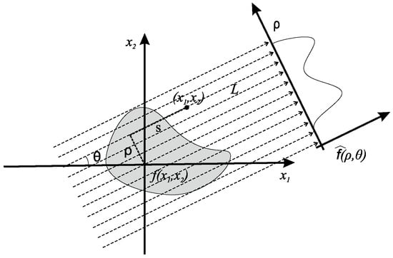
Figure 1.
Cartesian geometry of the Radon transform.
As Equation (1) suggests, analytic PET reconstructions entail the inversion of the Radon transform. In this direction, it has been established in [15,16] that the inverse Radon transform is given by the following expression:
where denotes the Hilbert transform () of the sinogram, namely
and ∮ denotes principal value integral. For the numerical implementation of the inversion, we employ Chebyshev polynomials of the first kind [21]. To this end, we approximate the sinogram function by
where denotes Chebyshev polynomials of the first kind [26], i.e.,
and N denotes the maximum degree of the Chebyshev polynomial taken into account in the sum on the right-hand-side of Equation (6). Taking into account Equation (6), Equation (5) may be rewritten as
Proposition 2.3(i) and Equation (2.17) of [27] suggest that:
where denotes the integer part of a real number a, while the primed sum implies that the last term of the sum must be halved when n is odd. Inserting Equation (9) in Equation (8) yields:
2.2. Numerical Implementation of the Inversion of the Radon Transform via Chebyshev Polynomials
For the evaluation of all quantities involved in the inversion Equation (4), we assume that is given for K projection angles, , and for detector locations, , namely:
The values of represent the roots of the Chebyshev polynomial , hence they belong to the zero set of , denoted by ,
Equation (7) implies that must be located in
Taking into account the above assumptions, we present the computational steps of our proposed, Chebyshev-based reconstruction algorithm in Algorithm 1.
| Algorithm 1: Computational steps of the proposed Chebyshev-based reconstruction algorithm |
| Reconstruction algorithm: Chebyshev approximation of the sinogram |
| Input: given at and |
| Compute: for all , and , via Equation (2), for all , and , via Equation (2), for all n, via Equation (7), for all n, via Equation (12), for all n, via Equation (6) as in [28], for all and , for all and , for all and , for all , and , , , via numerical integration |
| Output: |
3. Materials and Methods
3.1. Phantom Study: Simulated Micro-PET IQ Phantom via the NEMA NU 4-2008 Protocol
For the purposes of our studies, we simulated an image quality (IQ) phantom in the open-source library STIR (Software for Tomographic Image Reconstruction) [29], following the “NEMA NU 4-2008 standards” protocol for the performance measurements of small animal PET [23]. The IQ phantom is a poly(methyl methacrylate) (PMMA) cylindric container with internal dimensions of 50 mm in length and 30 mm in diameter, and comprises three main regions: (i) a uniform cylindrical chamber 30 mm in diameter and 30 mm in length, (ii) a 20 mm long solid region, containing five fillable rods with diameters of 1 mm, 2 mm, 3 mm, 4 mm, and 5 mm, respectively, and (iii) a lid supporting two, equally-sized, cold region chambers of 14 mm in length and 8 mm in diameter, filled with non-radioactive water and air, respectively. The phantom grid size employed was 119 × 119 × 161.
3.2. Sinograms
All sinograms, denoted by as in Equation (1), of the simulated IQ phantom described above were generated in MATLAB® R2019b (The Mathworks Inc., Natick, MA, USA). In particular, all sinograms involved had dimensions of 119 × 180 pixels, corresponding to 119 detectors and 180 angles (180 views over 180 degrees), respectively, with a bin size of 1.17 mm and 161 image slices. For the purposes of our Chebyshev and FBP-based simulations we created two types of sinograms: sinograms with equally spaced for FBP reconstructions, and sinograms evaluated in locations corresponding to the roots of the Chebyshev polynomials, as in Equation (15). The simulated sinograms were acquired for three noise levels (NL), taking into account 100% (NL1), 50% (NL2) and 20% (NL3) of the total counts, respectively. The noisy sinograms were generated by adding Poisson noise in ten realizations () at each of the three noise levels.
3.3. Reconstructions
The reconstructions of all sinograms were performed with our Chebyshev-based method and with FBP, and were implemented in Matlab. The reconstruction grid for the reconstructed images generated by both reconstruction algorithms was 119 × 119 × 161 pixels, corresponding to scale factors of 1.17, 1.17 and 0.585 mm/pixel, respectively. For the FBP reconstructions, a ramp filter was applied with a cut-off frequency equal to the Nyquist frequency. In our computations, we chose to take Chebyshev polynomials, , up to N = 119, i.e., equal to the number of the total segments of the domain, available from the sinogram. The reason for this selection is dictated by the mathematics of Chebyshev polynomials. More specifically, when interpolating via Equation (6), we take into account that the number of points available, located at the roots of the corresponding Chebyshev polynomial, are , as in Equations (13) and (15). Furthermore, when choosing N in this fashion, the approximation Formula (6) is exact for equal to the N zeros of , as in Section 5.8 of [28]. Initially, for both Chebyshev and FBP reconstructions, no post-reconstruction filtering was applied. However, in order to fairly compare the algorithms at equal noise levels, we also employed Gaussian post-reconstruction filtering in the reconstructions of NL3. In this direction, all images corresponding to NL3 (20% of the total counts) were blurred in Matlab with a Gaussian smoothing kernel of three different standard deviations, namely 0.5×, 1×, and 1.5× sigma. NL3 was selected for further filtering, as in [18], since it corresponds to the noise level of FBP for acquisition duration of 1200 s, which is the suggested acquisition duration according to the NEMA protocol [23].
3.4. Image Metrics
For the evaluation of our reconstructions, we employed the following image quality metrics: (i) percentage standard deviation (), (ii) recovery coefficient (), and (iii) spill-over ratio (), corresponding to the uniform, “hot” and “cold” regions of the IQ phantom, respectively.
3.4.1. Percentage Standard Deviation
The percentage standard deviation, denoted by , is related with the uniform cylindrical chamber of the phantom and is defined as the standard deviation divided by the mean multiplied by 100%, namely:
where and denote the standard deviation and mean, respectively, of the pixel values in the uniform region of the simulated phantom. In the “NEMA NU 4-2008 standards” protocol [23], is described as a measure of image uniformity (image noise).
3.4.2. Recovery Coefficient
The recovery coefficient, denoted by , is defined as the measured activity concentration in each hot fillable rod of the IQ phantom, divided by the mean activity concentration in the uniform cylindrical chamber, namely:
where and denote the average measured counts in the region-of-interest (ROI) corresponding to each hot rod, , and in the uniform area, respectively, and and denote the actual counts in the ROI corresponding to each hot rod, , and in the uniform area, respectively. The measurements corresponding to Equation (17) are averaged over all realizations, R, namely:
where and denote the measured counts in the ROI corresponding to the hot rod i and the uniform region, respectively, in the realization r. It is worth noting that the recovery coefficient () quantifies the “activity recovery” in environments with zero activity background [30], therefore is indicative of the spatial resolution of the imaging system [31,32,33,34]. The values of vary between 0 and 1. Furthermore, we note that, in the literature, the recovery coefficient is also referred to as “hot recovery coefficient” [35], similar to the so-called contrast recovery coefficient [36].
It is worth noting that for the calculations related to the simulated IQ phantom, we have followed the methodology of the NEMA protocol [23]. In particular, according to the NEMA protocol, the image slices covering the central 10 mm in length of the five fillable rods were averaged, in order to obtain a single image slice of lower noise. Around each fillable rod, circular ROIs with diameters twice the physical diameter of the rods were drawn in the averaged image. The maximum values in each of these ROIs were measured. The transverse image pixel coordinates of the locations with the maximum ROI values were recorded and used to create line profiles along the five fillable rods in the axial direction. The pixel values measured along each axial line profile, divided by the mean activity concentration found in the uniform cylindrical chamber of the phantom, were used to determine the mean of the for each rod size.
3.4.3. Spill-Over Ratio
The spill-over ratio, denoted by , is defined as the activity concentration in each cold cylinder divided by the mean activity concentration in the (hot) uniform cylindrical chamber of the IQ phantom:
where and denote the average measured counts in the region-of-interest (ROI) corresponding to each cold rod, , and in the uniform area, respectively. As in the case of where the measurements are perceived in terms of Equation (18), measurements are averaged over all realizations, R, i.e.,
where denotes the measured counts in the ROI corresponding to the cold cylinder i in the realization r. We note that with the spill-over ratio, we are provided with a measure of the imaging system’s ability to implement scatter correction [23].
3.4.4. Image Analysis
All reconstructed images of the simulated IQ phantom were analyzed with Image Quality Center (ver. 5.01), a Matlab-based software provided by Mediso Medical Imaging Systems [37]. This software calculates the image quality metrics: , , and as described above, per the “NEMA NU 4-2008 standards” protocol [23]. It is worth mentioning that each metric, x, evaluated, was presented in the following form:
where denotes the mean of x, denotes the so-called standard error of the mean [39], given by
denotes the standard deviation of the metric x, and R represents the total number of realizations.
4. Results
For the simulated NEMA IQ phantom, reconstructed images using Chebyshev and FBP for all noise levels are presented in Figure 2. The figure was created in the free software tool for multimodality medical image analysis AMIDE [40]. The reconstructions depicted in this figure are representative reconstructions of one out of ten Poisson noise realizations at all noise levels, namely NL1, NL2 and NL3, since no visual differences were apparent between the realizations simulated. In Figure 2, scalar values are represented accordingly in the colorbar, namely zero values are represented by the all-black color, whereas the maximum values of the simulated IQ phantom by the all-white color. By visual comparison, the FBP reconstructed images appear of higher noise than the Chebyshev reconstructed images. Furthermore, in Figure 3 we present the line profiles of the IQ phantom, in its uniform and cold regions, respectively, for all noise levels.
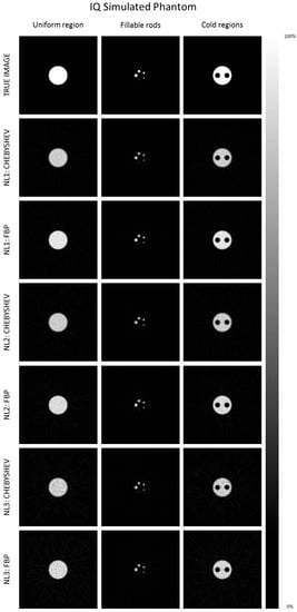
Figure 2.
Reconstructions of the simulated IQ phantom via Chebyshev and FBP, for NL1, NL2, and NL3.
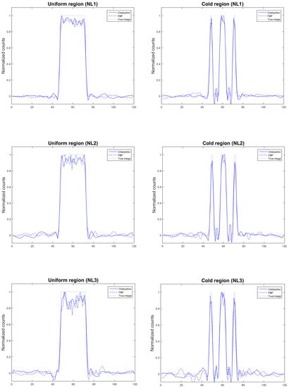
Figure 3.
Line profiles of the IQ phantom, in its uniform (left) and cold (right) regions, for all noise levels.
In Table 1, we present the percentage standard deviation () measurements in all noise levels, for both Chebyshev and FBP reconstructions. The images reconstructed via Chebyshev exhibited considerably lower noise, compared to the ones reconstructed via FBP, in all noise levels. We note that the measurements in NL3 for FBP agree with the corresponding measurements in [18]. In this direction, the FBP level of noise in our measurements in NL3 is consistent with the one corresponding to FBP for acquisition duration of 1200 s, recommended by the NEMA protocol [23].

Table 1.
Percentage standard deviation () measurements for the uniform region of the simulated IQ phantom for Chebyshev and FBP reconstructions, for all noise levels.
Figure 4 illustrates the recovery coefficient, , calculated for each of the five hot rods in the hot region of the simulated IQ phantom, namely for the rods with diameters of 1 mm, 2 mm, 3 mm, 4 mm, and 5 mm, respectively. The values are plotted for all three noise levels, and for Chebyshev and FBP reconstructions. We observe that the FBP reconstructions present slightly higher values than the Chebyshev ones in the expense of higher noise. Furthermore, we observe that the is independent of the noise level, as expected. It is worth noting that in the Chebyshev-based reconstructions, the recovery coefficient values for the hot rods with diameters 4 and 5 mm are larger than 1. This overestimation is not uncommon in PET, and is usually accepted by several commercial preclinical systems, including the Mediso nanoScan® PC small-animal PET/CT scanner used in [18,37]. values greater than 1 are due to few-pixel measurements from the average image, generated by averaging larger axial regions, especially in cases were small, pointlike sources are located inside regions with no background activity [41].
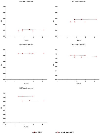
Figure 4.
Recovery coefficient () measurements for each of the hot fillable rods (diameters 1 to 5 mm) of the simulated IQ phantom, over the percentage standard deviation (), for Chebyshev and FBP reconstructions, corresponding to all noise levels. Note that the leftmost data point in each curve corresponds to NL1 (less noise), whereas the rightmost data point corresponds to the NL3 case.
In Figure 5, we illustrate the values as a function of the five rod diameters of the simulated IQ phantom, namely 1 mm, 2 mm, 3 mm, 4 mm and 5 mm, for both reconstruction methods investigated. This specific plot may be referred to as the recovery coefficient curve. As shown in Figure 5, Chebyshev reconstructions exhibited similar values with FBP for the hot rods with diameters 1 to 3 mm, whereas for the hot rods with diameters 4 and 5 mm exhibited higher values. The values decrease as the rod size decreases for both algorithms [41,42].
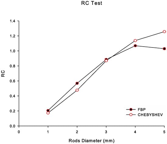
Figure 5.
Recovery coefficient () for all hot fillable rods in the hot region of the simulated IQ phantom as a function of rod diameter (in mm), for Chebyshev and FBP reconstructions in NL2.
In Figure 6, we present the spill-over ratio () measurements for the water-filled and the air-filled chambers in the cold region of the simulated IQ phantom, for all noise levels, and for Chebyshev and FBP reconstructions. We observe that the impact of in is minimal. It is worth mentioning that in both Figure 5 and Figure 6, the small standard error of the mean (SEM) bars indicate that the variation of the mean values is negligible in the metrics evaluated, namely and .
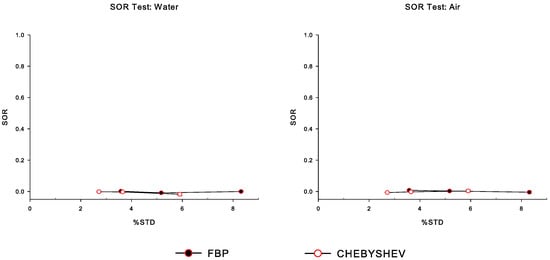
Figure 6.
Spill-over ratio () measurements for the two water-filled and air-filled chambers in the cold region of the simulated IQ phantom, over the percentage standard deviation (), for Chebyshev and FBP reconstructions, corresponding to all noise levels. Note that the leftmost data point in each curve corresponds to NL1 (less noise), whereas the rightmost data point corresponds to the NL3 case.
Furthermore, in Table 2 we present the measurements, resulting from the combination of the corresponding ones of and . As shown in Table 2, Chebyshev reconstructions exhibited consistently higher values than FBP, for all hot rods and for all noise levels investigated.

Table 2.
Contrast-to-noise-ratio () measurements for the hot region of the simulated IQ phantom for Chebyshev and FBP reconstructions, for all hot fillable rods, for all noise levels.
Figure 7 illustrates the versus plots, for each of the hot fillable rods (diameters 1 to 5 mm) of the simulated IQ phantom, for Chebyshev and FBP reconstructions, corresponding to all sigma values, namely from right to left: NL3 (no smoothing), 0.5×, 1×, and 1.5× sigma, respectively. We observe that, for all rod sizes, Chebyshev-based reconstructions exhibit higher values for between 3% to 6%, whereas, for between 1% to 2%, FBP reconstructions have higher values than the corresponding ones of Chebyshev. As expected, more Gaussian smoothing (larger sigma) leads to lower as well as values.
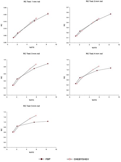
Figure 7.
Recovery coefficient () measurements for each of the hot fillable rods (diameters 1 to 5 mm) of the simulated IQ phantom, as functions of percentage standard deviation (), for Chebyshev and FBP reconstructions, corresponding to all sigma values, namely from right to left: NL3 (no smoothing), 0.5×, 1×, and 1.5× sigma, respectively.
Finally, in Figure 8 we have plotted versus , for the water-filled and air-filled chambers in the cold region of the simulated IQ phantom, for Chebyshev and FBP reconstructions, corresponding to all sigma values, namely from right to left: NL3 (no smoothing), 0.5×, 1×, and 1.5× sigma, respectively. We observe that the calculated values for both analytic reconstruction algorithms are similar. As expected, for both FBP and Chebyshev reconstructions, the value increases as the increases.
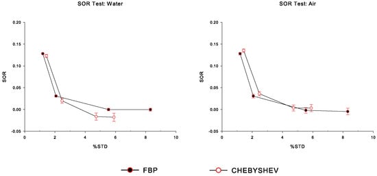
Figure 8.
Spill-over ratio () measurements for the water-filled and air-filled chambers in the cold region of the simulated IQ phantom, as functions of percentage standard deviation (), for Chebyshev and FBP reconstructions, corresponding to all sigma values, namely from right to left: NL3 (no smoothing), 0.5×, 1×, and 1.5× sigma, respectively.
5. Discussion
In this work we have presented a new analytic reconstruction technique based on Chebyshev polynomials of the first kind, and have evaluated it, in comparison to the analytic industry-standard method of FBP, in a simulated IQ phantom according to the NEMA NU 4-2008 protocol. For the evaluation of the performance of our new method, we employed several image metrics, including the percentage standard deviation for the uniform region of the phantom, the recovery coefficient for the hot region of the phantom and the spill-over ratio for the cold region of the phantom. Our results suggest that our Chebyshev-based reconstruction algorithm is capable of producing accurate analytic reconstructions for the simulated IQ phantom.
It is important to note that the main hypotheses involved in our current work are supported by our findings. Firstly, the hypothesis that Chebyshev polynomials of the first kind operate exclusively in the physical space, without incorporating the Fourier transform, which is expected to benefit the contrast of the reconstructed images. Secondly, the fact that Chebyshev polynomials operate globally, instead of locally, when interpolating the sinogram, which proved to be beneficial in terms of noise in the reconstructed images. Furthermore, we note that Chebyshev polynomials for PET reconstruction have similar computational efficiency to other analytical reconstruction formulations, such as SRT (based on splines), as in [18], where a thorough comparison of the spline technique with FBP has been performed following the same NEMA protocol. Chebyshev had similar computation complexity to other polynomial-based analytical transformations [16], however simpler transformations like FBP are less computationally expensive.
In particular, for the uniform region of the simulated IQ phantom, our new analytic method provided images with percentage standard deviation () considerably lower than FBP in all noise levels investigated. In the uniform region, Chebyshev reconstructions were consistently improved over FBP, in terms of percentage standard deviation (up to 29% lower values, depending on the noise level). For the hot regions of the simulated IQ phantom, our Chebyshev-based method provided images with recovery coefficients similar to FBP in the rods with diameter 1, 2 and 3 mm, whereas higher values in the rods with diameter 4 and 5mm. When post-smoothing was applied, in order to compare at similar noise levels, Chebyshev demonstrated values up to 14% and 42% higher, for rods 1–3 mm and 4–5 mm, respectively, compared to FBP, depending on the smoothing sigma values. Especially in the cases of the 4 and 5 mm rods, values were overestimated and above 1. However, the measured contrast-to-noise-ratio indicated an improvement of Chebyshev versus FBP of up to 68%, depending on the noise level. Our measurements provide a better indication of the advantages of Chebyshev reconstructions. Furthermore, at equal noise levels, namely between 3% to 6%, higher values were achieved via Chebyshev, whereas at lower noise levels FBP seems to have an advantage. For the cold regions of the simulated IQ phantom, Chebyshev provided images with spill-over ratios similar to FBP in the water-filled and air-filled chambers. In the measurements, there occurred several negative values. This is due to the fact that analytic methods are expected to produce negative values in pixels where the corresponding phantom value is either very low or zero [17,43].
6. Conclusions
In the present study we have presented a new mathematical formulation for the analytical inversion of the Radon transform and its corresponding numerical implementation based on Chebyshev polynomials of the first kind. We have tested our algorithm on a simulated IQ phantom and compared our results with FBP, the industry-standard analytic reconstruction method in PET. For the evaluation of our simulated studies based on Chebyshev polynomials of the first kind, we employed the “NEMA NU 4-2008 standards” protocol. Our results indicate that our Chebyshev-based reconstruction technique is comparable with FBP, probably providing a good analytic alternative for two dimensional reconstructions. In future studies, we aim to investigate the performance of our analytic reconstruction algorithm in clinical PET studies, especially as it compares with FBP and ordered subsets expectation maximization (OSEM).
Author Contributions
Conceptualization, N.E.P., A.S.F., V.M. and G.A.K.; methodology, N.E.P., V.M. and G.A.K.; software and validation, N.E.P., A.V., N.D. and G.A.K.; writing—original draft preparation, N.E.P.; writing—review and editing, N.E.P., A.S.F., A.V., V.M., N.D. and G.A.K.; visualization, N.E.P., A.V. and N.D.; supervision, G.A.K. All authors have read and agreed to the published version of the manuscript.
Funding
This research was partially supported by the research programme No. 200/948 of the Research Committee of the Academy of Athens.
Institutional Review Board Statement
Not applicable.
Informed Consent Statement
Not applicable.
Data Availability Statement
The data presented in this study are available on request from the corresponding author.
Conflicts of Interest
The authors declare no conflict of interest.
References
- Aulakh, G.K.; Kaur, M.; Brown, V.; Ekanayake, S.; Khan, B.; Fonge, H. Quantification of regional murine ozone-induced lung inflammation using [18F]F-FDG microPET/CT imaging. Sci. Rep. 2020, 10, 15699. [Google Scholar] [CrossRef] [PubMed]
- Kollenda, S.A.; Klose, J.; Knuschke, T.; Sokolova, V.; Schmitz, J.; Staniszewska, M.; Costa, P.F.; Herrmann, K.; Westendorf, A.M.; Fendler, W.P.; et al. In vivo biodistribution of calcium phosphate nanoparticles after intravascular, intramuscular, intratumoral, and soft tissue administration in mice investigated by small animal PET/CT. Acta Biomater. 2020, 109, 244–253. [Google Scholar] [CrossRef] [PubMed]
- Iancu, S.D.; Albu, C.; Chiriac, L.; Moldovan, R.; Stefancu, A.; Moisoiu, V.; Coman, V.; Szabo, L.; Leopold, N.; Bálint, Z. Assessment of gold-coated iron oxide nanoparticles as negative T2 contrast agent in small animal MRI studies. Int. J. Nanomed. 2020, 15, 4811. [Google Scholar] [CrossRef] [PubMed]
- Sivasubramanian, K.; Periyasamy, V.; Pramanik, M. Non-invasive sentinel lymph node mapping and needle guidance using clinical handheld photoacoustic imaging system in small animal. J. Biophotonics 2018, 11, e201700061. [Google Scholar] [CrossRef]
- Johnson, L.C.; Guerraty, M.A.; Moore, S.C.; Metzler, S.D. Quantification of myocardial uptake rate constants in dynamic small-animal SPECT using a cardiac phantom. Phys. Med. Biol. 2019, 64, 065018. [Google Scholar] [CrossRef]
- Liang, H.; Yang, Y.; Yang, K.; Wu, Y.; Boone, J.M.; Cherry, S.R. A microPET/CT system for in vivo small animal imaging. Phys. Med. Biol. 2007, 52, 3881. [Google Scholar] [CrossRef]
- Liu, Q.; Li, C.; Liu, J.; Krish, K.; Fu, X.; Zhao, J.; Chen, J.C. Performance evaluation of a small-animal PET/CT system based on NEMA NU 4–2008 standards. Med. Phys. 2021, 48, 5272–5282. [Google Scholar] [CrossRef]
- Yao, R.; Lecomte, R.; Crawford, E.S. Small-animal PET: What is it, and why do we need it? J. Nucl. Med. Technol. 2012, 40, 157–165. [Google Scholar] [CrossRef]
- Cherry, S.; Shao, Y.; Silverman, R.; Meadors, K.; Siegel, S.; Chatziioannou, A.; Young, J.; Jones, W.; Moyers, J.; Newport, D.; et al. MicroPET: A high resolution PET scanner for imaging small animals. IEEE Trans. Nucl. Sci. 1997, 44, 1161–1166. [Google Scholar] [CrossRef]
- Green, M.V.; Seidel, J.; Vaquero, J.J.; Jagoda, E.; Lee, I.; Eckelman, W. High resolution PET, SPECT and projection imaging in small animals. Comput. Med. Imaging Graph. 2001, 25, 79–86. [Google Scholar] [CrossRef]
- Kang, K.J.; Oh, S.J.; Nam, K.R.; Ahn, H.; Park, J.A.; Lee, K.C.; Choi, J.Y. Validation of Image Qualities of a Novel Four-Mice Bed PET System as an Oncological and Neurological Analysis Tool. J. Imaging 2021, 7, 43. [Google Scholar] [CrossRef] [PubMed]
- Nose, N.; Nogami, S.; Koshino, K.; Chen, X.; Werner, R.A.; Kashima, S.; Rowe, S.P.; Lapa, C.; Fukuchi, K.; Higuchi, T. [18F] FDG-labelled stem cell PET imaging in different route of administrations and multiple animal species. Sci. Rep. 2021, 11, 10896. [Google Scholar] [CrossRef] [PubMed]
- Tong, S.; Alessio, A.M.; Kinahan, P.E. Image reconstruction for PET/CT scanners: Past achievements and future challenges. Imaging Med. 2010, 2, 529–545. [Google Scholar] [CrossRef] [PubMed]
- Gong, K.; Kim, K.; Cui, J.; Wu, D.; Li, Q. The evolution of image reconstruction in PET: From filtered back-projection to artificial intelligence. PET Clin. 2021, 16, 533–542. [Google Scholar] [CrossRef] [PubMed]
- Fokas, A.; Iserles, A.; Marinakis, V. Reconstruction algorithm for single photon emission computed tomography and its numerical implementation. J. R. Soc. Interface 2006, 3, 45–54. [Google Scholar] [CrossRef]
- Kastis, G.A.; Kyriakopoulou, D.; Gaitanis, A.; Fernández, Y.; Hutton, B.F.; Fokas, A.S. Evaluation of the spline reconstruction technique for PET. Med. Phys. 2014, 41, 042501. [Google Scholar] [CrossRef]
- Kastis, G.A.; Gaitanis, A.; Samartzis, A.P.; Fokas, A.S. The SRT reconstruction algorithm for semiquantification in PET imaging. Med. Phys. 2015, 42, 5970–5982. [Google Scholar] [CrossRef]
- Vrachliotis, A.; Kastis, G.A.; Protonotarios, N.E.; Fokas, A.; Nekolla, S.G.; Anagnostopoulos, C.D.; Costaridou, L.; Gaitanis, A. Evaluation of the spline reconstruction technique for preclinical PET imaging. Comput. Methods Programs Biomed. 2022, 217, 106668. [Google Scholar] [CrossRef]
- Protonotarios, N.E.; Fokas, A.S.; Kostarelos, K.; Kastis, G.A. The attenuated spline reconstruction technique for single photon emission computed tomography. J. R. Soc. Interface 2018, 15, 20180509. [Google Scholar] [CrossRef]
- Bortfeld, T.; Oelfke, U. Fast and exact 2D image reconstruction by means of Chebyshev decomposition and backprojection. Phys. Med. Biol. 1999, 44, 1105. [Google Scholar] [CrossRef]
- Fokas, A.S.; Marinakis, V. Reconstruction algorithm for the brain imaging techniques of PET and SPECT. HERMIS 2003, 4, 45–61. [Google Scholar]
- Bahri, M.A.; Plenevaux, A.; Warnock, G.; Luxen, A.; Seret, A. NEMA NU4-2008 image quality performance report for the microPET Focus 120 and for various transmission and reconstruction methods. J. Nucl. Med. 2009, 50, 1730–1738. [Google Scholar] [CrossRef] [PubMed][Green Version]
- NEMA. NEMA Standards Publication NU 4-2008: Performance Measurements of Small Animal Positron Emission Tomographs; Technical Report; National Electrical Manufacturers Association: Rosslyn, VA, USA, 2001. [Google Scholar]
- Barrett, H.H.; Myers, K.J. Foundations of Image Science; Wiley Series in Pure and Applied Optics; Wiley: Hoboken, NJ, USA, 2004. [Google Scholar]
- Fokas, A.S.; Kastis, G.A. Mathematical methods in PET and SPECT imaging. In Handbook of Mathematical Methods in Imaging; Scherzer, O., Ed.; Springer: New York, NY, USA, 2015; pp. 903–936. [Google Scholar] [CrossRef]
- Gil, A.; Segura, J.; Temme, N.M. Numerical Methods for Special Functions; SIAM: Philadelphia, PA, USA, 2007. [Google Scholar]
- Notaris, S. Integral formulas for Chebyshev polynomials and the error term of interpolatory quadrature formulae for analytic functions. Math. Comput. 2006, 75, 1217–1231. [Google Scholar] [CrossRef]
- Press, W.H.; Teukolsky, S.A.; Vetterling, W.T.; Flannery, B.P. Numerical Recipes 3rd Edition: The Art of Scientific Computing, 3rd ed.; Cambridge University Press: New York, NY, USA, 2007. [Google Scholar]
- Thielemans, K.; Tsoumpas, C.; Mustafovic, S.; Beisel, T.; Aguiar, P.; Dikaios, N.; Jacobson, M.W. STIR: Software for Tomographic Image Reconstruction release 2. Phys. Med. Biol. 2012, 57, 867–883. [Google Scholar] [CrossRef] [PubMed]
- Lajtos, I.; Czernin, J.; Dahlbom, M.; Daver, F.; Emri, M.; Farshchi-Heydari, S.; Forgacs, A.; Hoh, C.K.; Joszai, I.; Krizsan, A.K.; et al. Cold wall effect eliminating method to determine the contrast recovery coefficient for small animal PET scanners using the NEMA NU-4 image quality phantom. Phys. Med. Biol. 2014, 59, 2727. [Google Scholar] [CrossRef] [PubMed]
- Hoffman, E.J.; Huang, S.C.; Phelps, M.E. Quantitation in positron emission computed tomography: 1. Effect of object size. J. Comput. Assist. Tomogr. 1979, 3, 299–308. [Google Scholar] [CrossRef]
- Kessler, R.M.; Ellis, J.R., Jr.; Eden, M. Analysis of emission tomographic scan data: Limitations imposed by resolution and background. J. Comput. Assist. Tomogr. 1984, 8, 514–522. [Google Scholar] [CrossRef]
- Zhu, Y.; Geng, C.; Huang, J.; Liu, J.; Wu, N.; Xin, J.; Xu, H.; Yu, L.; Geng, J. Measurement and evaluation of quantitative performance of PET/CT images before a multicenter clinical trial. Sci. Rep. 2018, 8, 9035. [Google Scholar] [CrossRef]
- Srinivas, S.M.; Dhurairaj, T.; Basu, S.; Bural, G.; Surti, S.; Alavi, A. A recovery coefficient method for partial volume correction of PET images. Ann. Nucl. Med. 2009, 23, 341–348. [Google Scholar] [CrossRef]
- Bettinardi, V.; Danna, M.; Savi, A.; Lecchi, M.; Castiglioni, I.; Gilardi, M.C.; Bammer, H.; Lucignani, G.; Fazio, F. Performance evaluation of the new whole-body PET/CT scanner: Discovery ST. Eur. J. Nucl. Med. Mol. Imaging 2004, 31, 867–881. [Google Scholar] [CrossRef]
- Tong, S.; Alessio, A.M.; Kinahan, P.E. Noise and signal properties in PSF-based fully 3D PET image reconstruction: An experimental evaluation. Phys. Med. Biol. 2010, 55, 1453–1473. [Google Scholar] [CrossRef] [PubMed]
- Gaitanis, A.; Kastis, G.A.; Vlastou, E.; Bouziotis, P.; Verginis, P.; Anagnostopoulos, C.D. Investigation of image reconstruction parameters of the Mediso nanoScan PC small-animal PET/CT scanner for two different positron emitters under NEMA NU 4-2008 standards. Mol. Imaging Biol. 2017, 19, 550–559. [Google Scholar] [CrossRef] [PubMed]
- Visser, E.P.; Disselhorst, J.A.; van Lier, M.G.; Laverman, P.; de Jong, G.M.; Oyen, W.J.; Boerman, O.C. Characterization and optimization of image quality as a function of reconstruction algorithms and parameter settings in a Siemens Inveon small-animal PET scanner using the NEMA NU 4-2008 standards. Nucl. Instrum. Methods Phys. Res. Sect. A Accel. Spectrom. Detect. Assoc. Equip. 2011, 629, 357–367. [Google Scholar] [CrossRef]
- Altman, D.G.; Bland, J.M. Standard deviations and standard errors. BMJ 2005, 331, 903. [Google Scholar] [CrossRef] [PubMed]
- Loening, A.M.; Gambhir, S.S. AMIDE: A free software tool for multimodality medical image analysis. Mol. Imaging 2003, 2, 131–137. [Google Scholar] [CrossRef]
- Goertzen, A.L.; Bao, Q.; Bergeron, M.; Blankemeyer, E.; Blinder, S.; Cañadas, M.; Chatziioannou, A.F.; Dinelle, K.; Elhami, E.; Jans, H.S.; et al. NEMA NU 4-2008 comparison of preclinical PET imaging systems. J. Nucl. Med. 2012, 53, 1300–1309. [Google Scholar] [CrossRef]
- Luo, W.; Anashkin, E.; Matthews, C.G. Performance evaluation of a PEM scanner using the NEMA NU 4—2008 small animal PET standards. IEEE Trans. Nucl. Sci. 2010, 57, 94–103. [Google Scholar] [CrossRef]
- O’Sullivan, F.; Pawitan, Y.; Haynor, D. Reducing negativity artifacts in emission tomography: Post-processing filtered backprojection solutions. IEEE Trans. Med. Imaging 1993, 12, 653–663. [Google Scholar] [CrossRef]
Publisher’s Note: MDPI stays neutral with regard to jurisdictional claims in published maps and institutional affiliations. |
© 2022 by the authors. Licensee MDPI, Basel, Switzerland. This article is an open access article distributed under the terms and conditions of the Creative Commons Attribution (CC BY) license (https://creativecommons.org/licenses/by/4.0/).