Featured Application
In this paper, we put forward a novel modulation format identification (MFI) technique for a free-space optical (FSO) communication system based on a convolution neural network (CNN). The random parameters training method we use can improve the robustness against atmospheric optical turbulence and additive Gaussian white noise (AWGN). The proposed MFI scheme in this paper is a viable solution in the application of an FSO communication simulation channel, which can easily deal with the scene of fast modulation format switching and accurate identification to satisfy system requirements. Therefore, we hope that the MFI scheme we proposed is able to find a practical application in satellite-to-ground FSO systems.
Abstract
The satellite-to-ground communication system is a significant part of future space communication networks. The free-space optical (FSO) communication technique is a prospective solution for satellite-to-ground communication. However, atmospheric optical turbulence is a major impairment in FSO communication systems. In this paper, to improve the performance and flexibility of a satellite-to-ground laser communication system, we put forward a novel modulation format identification (MFI) technique for an FSO communication system based on a convolution neural network (CNN). The results indicate that our CNN model can blindly and accurately identify the modulation format with classification accuracy up to 99.98% for random channel condition, including the strength of turbulence and signal-to-noise ratio (SNR) of additive Gaussian white noise (AWGN) ranging from 10dB to 30dB. Moreover, the CNN demonstrated robustness against atmospheric optical turbulence and suggested immunity to additive noise. Therefore, the proposed methodology proved to be a viable solution in the application of an FSO communication simulation channel, which can easily deal with the scene of fast modulation format switching and accurate identification to satisfy system requirements. Therefore, we hope this scheme can find a practical implementation in satellite-to-ground optical wireless systems.
1. Introduction
The satellite-to-ground communication system is a significant part of future space communication networks. Radio frequency (RF) communication links for inter-satellite or satellite-to-ground communication are increasingly limited due to the unideal spectrum availability and limited data rate. A free-space optical (FSO) communication system has become one of the most promising technologies in future communication systems because of it being superior to the traditional RF system [1]. At present, FSO communication links are beginning to take over RF communication links in the field of high bandwidth applications [2]. The requirement tendency of forthcoming satellite data transmission has grown to become a critical boost to the progress of communication technology. Gigantic amounts of information and complicated channel circumstances require high data speed and flexibility at the same time. FSO communication has been taking part in a more vital role in the satellite-to-ground communication step by step [3]. For the flexibility of services and applications, the next-generation FSO network is expected to adjust the modulation format dynamically according to the link conditions and terminal equipment configuration to meet the different requirements of the terminal system and service [4,5]. The traditional method needs to spend time and data processing prior information from the transmitter in the recognition process, which is a great waste in the short connection time of a satellite-to-earth link. To promote demodulation efficiency, it is a challenging requirement for an FSO receiver to realize blind modulation format identification (MFI). Over the last few years, several classical MFI techniques for optical communication have been proposed [6,7,8].
Machine learning (ML) is a powerful interdisciplinary subject combining mathematics, computing, and biological sciences. In recent years, it has been successfully applied in the fields of pattern recognition, computer vision, personalized technology, and data analysis and mining [9]. Recently, techniques from ML have also performed well in some intelligent expansion directions in the field of optical communication, such as optical performance monitoring (OPM), MFI, and nonlinear impairments compensation [4,9,10]. Compared with traditional methods, the advantage of ML methods for MFI is that it completes the training of the model before practical application [11]. It only needs to let the model know all possible modulation formats during training. In practical use, it can quickly obtain reliable recognition results without sacrificing the processing of prior information. Before that, if the results are not satisfactory in the training process, the model parameters can be adjusted repeatedly before actual communication without adjusting in the time after the actual link is established. As a representative algorithm of machine learning, convolutional neural networks (CNN) have made great achievements in image recognition. Sparse connectivity allows CNN to recognize the local features of input images without all connected feature engineering, which makes CNN distinctly efficient from conventional machine learning techniques [12]. Also, the results of paper [9] show that CNN achieves optimal accuracy and is significantly superior to other ML methods.
However, previous research on MFI has focused mainly on radio and fiber-optic communication networks, and not as much work has been done for MFI in FSO communication networks [13,14]. In this paper, we focus on the performance of the CNN algorithm in modulation format recognition in an FSO communication system. Here, we mainly illustrate an FSO optical communication system under the random channel condition including the strength of atmosphere turbulence and signal-to-noise ratio (SNR) of AWGN. Four modulation formats were adopted in this paper: (1) On-Off Keying (OOK), (2) Binary Phase Shift Keying (BPSK), (3) Quadrature Phase Shift Keying (QPSK), and (4) 16-Quadrature Amplitude Modulation (16-QAM).
The rest of this paper is organized as follows: Section 2 indicates an overview of CNN’s theoretical background. Channel statistics with a gamma-gamma model is dissected in Section 3. The experimental process and the structure of network we designed are introduced in detail in Section 4. Finally, some results and discussions are maintained in Section 5, and conclusions are in Section 6.
2. CNN Theoretical Background
CNN is a kind of deep neural network (DNN) that is composed of input layer, hidden layer, and Full-Connected (FC) layer [15]. The hidden layer is a layer with different function, such as convolution layer, Batch Normalization (BN) layer, activation layer, and pooling layer. Generally, a typical structure of CNN is composed of many blocks connected between input and output, in which each block comprises one or several hidden layers [16,17]. An FC layer and a classification layer follow the last block and are finally connected to the output layer. A basic network structure is shown in Figure 1.
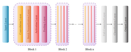
Figure 1.
Typical fully connected CNN network architecture.
The convolution layer extracts the feature data from the input data by convolution, to change the data processing of the neural network from a single point to different regions and complete data dimensionality reduction. It contains many convolution kernels, which can be regarded as filters. Each element of convolution kernels corresponds to a weight and a bias. When the convolution kernel windows slide on the input data matrix, the filter can convolute with the local data.
Next, the matrix enters the BN layer to convert the data to the same order of magnitude. Then, the matrix enters the activation layer to increase the nonlinearity of the neural network model, so that the neural network can better fit with more kinds of curves and better solve more complex problems. In this paper, we use the rectified linear unit (ReLU) function as the activation function. For the pooling layer, after the input data is divided into many rectangular regions, the output value of each subregion is represented as one point to reduce the dimension for feature extraction. Here, we use the two most common pooling layers, the maximum pooling layer, and the average pooling layer.
Before the final classification decision, the FC layer is used to connect each neuron with each neuron in the previous layer. After the feature map is generated to an appropriate dimension, all neurons are weighted into the FC layer, which can ignore the impact of spatial structure and reduce the impact of location on classification. By activating the classification, the output layer can output the calculated classification results. This article uses the most common Softmax function here, therefore, the probability of each type is mapped to the positive range, and then normalized to (0,1) to obtain the probability of each category. Finally, the output layer outputs the classification decision.
3. Channel Statistics with Gamma-Gamma Model
In FSO system, one of the main impairments is atmospheric optical turbulence, which can cause scintillation. Scintillation-induced fading adversely affects FSO links and damages its communication performance. The scintillation results from the index of refraction fluctuations in the atmosphere, which can cause random fluctuations of the received signal intensity and severely reduce the level of the optical signal. The statistics of the scintillation strength is usually regarded as following the gamma-gamma distribution, which is applicable to all turbulence situations from weak to strong. This model, proposed in [18], is based on the modulation process, in which the optical radiation fluctuation through turbulent atmosphere is assumed to be composed of small-scale (scattering) and large-scale (refraction) effects. Therefore, the normalized received irradiance is defined as the product of two statistically independent random processes and .
and are generated by the large-scale and small-scale turbulent eddies, respectively, and both obey the gamma distribution given by [19]. Consequently, their probability density functions (PDF) are given by
By fixing and using the change of variable, , the conditional PDF given by Equation (4) is obtained, in which is the (conditional) mean value of .
To obtain the unconditional irradiance distribution, the conditional probability is averaged over the statistical distribution of given by Equation (2) to obtain the following gamma-gamma irradiance distribution function.
where and represent the effective number of large-scale and small-scale eddies in the scattering process, respectively. represents the gamma function, and is the modified Bessel function of the second kind of order . If the optical radiation at the receiver is assumed to be a plane wave, then the two parameters and that characterize the irradiance fluctuation PDF are related to the atmospheric conditions [18], as follows:
while the scintillation index is given by
Often, is the log irradiance variance for a plane wave [19], which is defined as
In Equation (9), is the refractive index structure parameter, which characterizes the atmospheric optical turbulence effect. Generally, the range varies from 10−15 m−2/3 to 10−12 m−2/3 for the weak to strong turbulence regime, respectively. The gamma-gamma turbulence model given by Equation (5), which is applicable to all turbulence strengths from weak to strong. The values of and under different turbulence regimes are depicted in Figure 2.
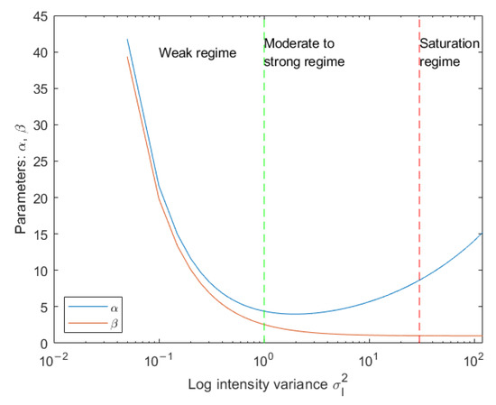
Figure 2.
Values of and under different turbulence regimes: weak, moderate to strong, and saturation.
In this work, we use three different turbulence regimes: weak, moderate to strong, and saturation, as depicted in Figure 3, with the parameters given in [19]. The , , and values for weak turbulence are 11.6, 10.1, and 0.2, respectively. The , , and values for moderate turbulence are 4, 1.9, and 1.6, respectively. The , , and values for strong turbulence are 4.2, 1.4, and 3.5, respectively.
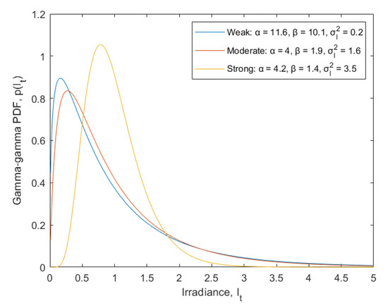
Figure 3.
Gamma-gamma probability density function for three different turbulence regimes, weak, moderate, and strong with different , , and values, respectively.
4. Simulation Setup
In this paper, the architecture of our system can be seen in Figure 4. The Communication and Deep Learning Toolbox in MATLAB Software is used for simulation. We chose four typical and promising modulation formats, OOK, BPSK, QPSK, and 16 QAM. A total of 20,000 frames are generated for each modulation format with a length of 1024 samples. Since the network makes each decision based on a single frame rather than multiple consecutive frames, such as video, each frame must pass through a separate channel. In the transmitter side, the input symbols to the system are sampled and transmitted by a gamma-gamma atmospheric channel with random strength, which ranges from weak to strong added to AWGN whose SNR is generated randomly. At the receiver, the received signal is
where, is the transmitted signal, is the gamma-gamma atmospheric channel, and is AWGN. Each frame contains 256 symbols, eight sampling points per symbol, and uses a gamma-gamma random variate. Therefore, a coherent time of atmospheric turbulence can be simulated. However, the AWGN is generated for each time step.
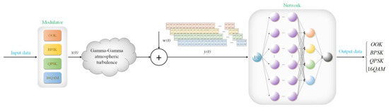
Figure 4.
Proposed optical communication system.
A random number of samples is removed from the beginning of each frame to remove transients and ensure that the frame has a random starting point relative to the symbol boundary. To improve the robustness against atmospheric optical turbulence and AWGN, random parameters are used to ensure the applicability of training data. We set the equals as 0.2, 1.6, and 3.5, representing the strength of turbulence of weak, moderate, and strong, respectively, for which the three parameter values have been used in most cases [18]. Additionally, we set the SNR of AWGN ranges from 10 to 30 dB. For a given turbulence regime, random fluctuations were added to the signal corresponding to of a particular turbulent regime to make sure all the data of every situation can be considered.
For the subsequent circumstance, the complex input is used as the input dimension of two real inputs, and is introduced into a narrow two-dimensional convolution network as a set of 2 × 1024 vectors, in which in-phase and quadrature sampling (I/Q) constitute this two-row data, which can be regarded as a two-dimensional image. Figure 5 and Figure 6 show the time domain diagrams and spectrograms of processed data for four modulation formats at present, respectively.
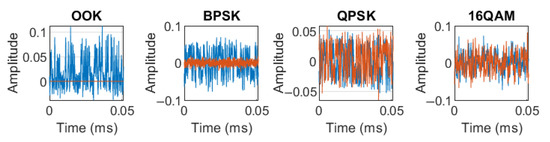
Figure 5.
Amplitude of the real and imaginary parts of the example frames against the sample number. The blue lines are for the real part, while the red ones are for the imaginary part. Weak turbulence with SNR = 10 is as an example above.
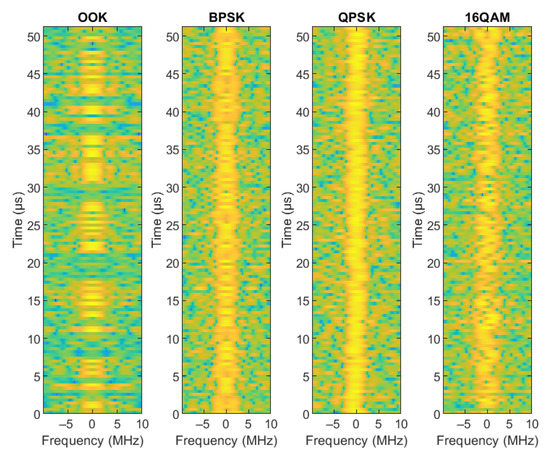
Figure 6.
Spectrogram of the example frames. Weak turbulence with SNR = 10 is as an example above.
In addition, Figure 7 shows the modulation constellation of the four modulation schemes when the SNR is 10 dB in the case of the weak turbulent channel as a typical example. It can be seen from the constellation points that the modulated signal has been disturbed by turbulence fluctuation and channel additive noise.
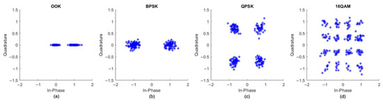
Figure 7.
Constellation diagram of (a) OOK, (b) BPSK, (c) QPSK, and (d) 16 QAM.
Next, the input data were separated into 80% for training, 20% for validation label accordingly. By ensuring that the number of tags for each modulation format is the same, class imbalance in training data is avoided. In this way, frames of four modulation formats were generated and channel-faded, and their corresponding tags stored and provided to the CNN network.
In the network structure adopted in this paper, six directly connected blocks are used. Each block is directly connected with four layers: convolution layer, BN layer, ReLU layer, and pooling layer. In the first five blocks, the maximum pooling layer is used to extract the meaningful features, and the average pooling layer is used in the last block to avoid erasing the details of the previous feature map. Finally, an FC layer is connected to the Softmax layer to output the classification decision. The network structure is shown in Figure 8 below.
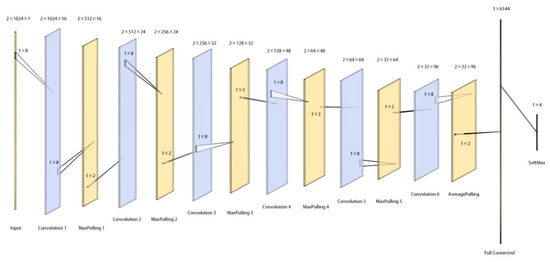
Figure 8.
Simplified network structure with feature matrix size and stride size.
The parameters of feature matrix size and stride size of major layers are listed in Table 1 below.

Table 1.
Network parameters of major layers.
After signal preprocessing, the synthesized signal is put into the CNN network whose structure is described in Section 2. Next, we use SGDM solver with the small batch size of 256. We set the maximum number of rounds to six, as more rounds will not provide further training advantage. The initial learning rate is set to 0.3, and the dropout rate is 0.6. After every four rounds, the learning rate will be reduced by a factor of 0.3. Specific parameters are listed in Table 2.
Table 2.
Network training parameters.
5. Results and Discussion
In the training process, verification is taken at the end of every epoch, and the final verification accuracy reaches over 99.99%. The training progress with accuracy and loss results is shown in Figure 9.
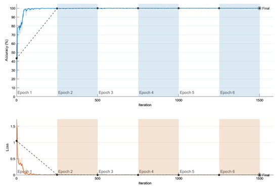
Figure 9.
Training progress with accuracy and loss results.
When the network training is successful, then the test process is carried out. Using the method of generating training data mentioned above, the random modulated data but with a different random seed is generated. Another 4000 test frames with random turbulence strength and AWGN with random SNR are generated for each format.
The trained network is used for recognition, and the test accuracy reaches over 99.99%. Three confusion matrix figures for the test data for three gamma-gamma turbulence strengths are shown in Figure 10. Figure 10a depicts the integrated test accuracy under different SNR (10–30 dB) in weak turbulent channels, and the test accuracy can reach 100%. Similarly, Figure 10b,c depict the moderate and strong turbulent channel circumstances, and the test accuracy can reach 99.9864% and 99.9818%, respectively. Moreover, Figure 11 shows the same meaning more intuitively.
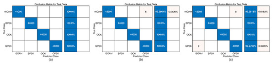
Figure 10.
Confusion matrix for test data for different turbulence strength: (a) weak, (b) moderate, and (c) strong.
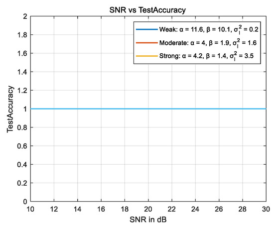
Figure 11.
SNR vs. test accuracy for weak, moderate, and strong turbulence strength.
6. Conclusions
This paper proposes a novel technique for MFI by applying a convolution neural network in an FSO link. Four widely used modulation formats (OOK, BPSK, QPSK, and 16 QAM) were comprehensively investigated. The recognition effect of our training network demonstrated robustness against atmospheric optical turbulence and suggested immunity to additive noise. Successful identification with over 99.98% test accuracy was achieved for studied scenarios.
Although the CNN algorithm achieved high recognition accuracy, the recognition accuracy cannot reach 100% when the modulation format types are similar. Therefore, in the future work, we hope to explore the application of recognition for more format types and feature-based data set construction, to improve the training time cost and accuracy. We believe that the proposed technique has the potential to be embedded in space networking and satellite-to-ground laser communication links.
Author Contributions
Writing—original draft preparation, Y.G.; Writing—review and editing, Y.G.; Visualization, X.L. and R.T.; Supervision, S.M. and T.J.; Project administration, Z.W. All authors have read and agreed to the published version of the manuscript.
Funding
This research received no external funding.
Institutional Review Board Statement
Not applicable.
Informed Consent Statement
Informed consent was obtained from all subjects involved in the study.
Data Availability Statement
This study did not report any data.
Acknowledgments
This work is supported by the Research Project of Scientific Research Equipment of Chinese Academy of Sciences. The authors also gratefully acknowledge the Optical Communication Laboratory of CIOMP for the use of their equipment.
Conflicts of Interest
The authors declare no conflict of interest.
References
- Khalighi, M.A.; Uysal, M. Survey on Free Space Optical Communication: A Communication Theory Perspective. IEEE Commun. Surv. Tutor. 2014, 16, 2231–2258. [Google Scholar] [CrossRef]
- Gong, S.; Shen, H.; Zhao, K. Network Availability Maximization for Free-Space Optical Satellite Communications. IEEE Wireless Commun. Lett. 2019, 9, 411–415. [Google Scholar] [CrossRef]
- Kaushal, H.; Kaddoum, G. Optical Communication in Space: Challenges and Mitigation Techniques. IEEE Commun. Surv. Tutor. 2017, 19, 57–96. [Google Scholar] [CrossRef] [Green Version]
- Musumeci, F.; Rottondi, C.; Nag, A.; Macaluso, I.; Tornatore, M. An overview on application of machine learning techniques in optical networks. IEEE Commun. Surv. Tutor. 2019, 21, 1383–1408. [Google Scholar] [CrossRef] [Green Version]
- Aveta, F.; Refai, H.H. Modulation format and number of users classification in multipoint free-space optical communication using convolutional neural network. Opt. Eng. 2020, 59, 060501. [Google Scholar] [CrossRef]
- Liu, J.; Dong, Z.; Zhong, K.; Lau, A.P.T.; Lu, C.; Lu, Y. Modulation format identification based on received signal power distributions for digital coherent receivers. In Proceedings of the Optical Fiber Communication Conference (OFC), San Francisco, CA, USA, 9–13 March 2014. [Google Scholar] [CrossRef]
- Borkowski, R.; Zibar, D.; Caballero, A.; Arlunno, V.; Monroy, I.T. Stokes Space-Based Optical Modulation Format Recognition for Digital Coherent Receivers. IEEE Photon. Technol. Lett. 2013, 25, 2129–2132. [Google Scholar] [CrossRef]
- Bilal, S.M.; Bosco, G.; Dong, Z.; Lau, A.P.T.; Lu, C. Blind modulation format identification for digital coherent receivers. Opt. Express 2015, 23, 26769–26778. [Google Scholar] [CrossRef] [PubMed] [Green Version]
- Wang, D.; Zhang, M.; Li, Z.; Li, J.; Fu, M.; Cui, Y.; Chen, X. Modulation Format Recognition and OSNR Estimation Using CNN-based Deep Learning. IEEE Photon. Technol. Lett. 2017, 29, 1667–1670. [Google Scholar] [CrossRef]
- Amirabadi, M.A.; Kahaei, M.H.; Nezamalhosseini, S.A.; Vakili, V.T. Deep learning for channel estimation in FSO communication system. Opt. Commun. 2019, 459, 124989. [Google Scholar] [CrossRef] [Green Version]
- Khan, F.N.; Zhong, K.; Al-Arashi, W.H.; Yu, C.; Chao, L.; Lau, A.P.T. Modulation Format Identification in Coherent Receivers Using Deep Machine Learning. IEEE Photon. Technol. Lett. 2016, 28, 1886–1889. [Google Scholar] [CrossRef]
- Li, J.; Zhang, M.; Wang, D.; Wu, S.; Zhan, Y. Joint atmospheric turbulence detection and adaptive demodulation technique using the CNN for the OAM-FSO communication. Opt. Express 2018, 26, 10494. [Google Scholar] [CrossRef] [PubMed]
- Liu, X.; Yang, D.; Gamal, A.E. Deep neural network architectures for modulation classification. In Proceedings of the 2017 51st Asilomar Conference on Signals, Systems, and Computers, Pacific Grove, CA, USA, 29 October–1 November 2017; pp. 915–919. [Google Scholar] [CrossRef] [Green Version]
- Xiang, Q.; Yang, Y.; Zhang, Q.; Yao, Y. Joint, accurate and robust optical signal to noise ratio and modulation format monitoring scheme using single Stokes-parameter-based artificial neural network. Opt. Express 2021, 29, 7276–7287. [Google Scholar] [CrossRef] [PubMed]
- Khan, F.N.; Fan, Q.; Lu, C.; Lau, A.P.T. Machine learning methods for optical communication systems and networks. In Optical Fiber Telecommunications, 7th ed.; Academic Press: Salty Lake City, UT, USA, 2020; pp. 921–978. [Google Scholar] [CrossRef]
- O’Shea, T.J.; Corgan, J.; Clancy, T.C. Convolutional Radio Modulation Recognition Networks. Commun. Comput. Inf. Sci. 2016, 213–226. [Google Scholar] [CrossRef] [Green Version]
- Darwesh, L.; Arnon, S. Deep learning for free space optics in a data center environment. Laser Communication and Propagation through the Atmosphere and Oceans VII. In Proceedings of the SPIE Optical Engineering + Applications, San Diego, CA, USA, 20–22 August 2018. [Google Scholar] [CrossRef]
- Andrews, L.C.; Philips, R.L.; Hopen, C.Y. Laser Beam Scintillation with Applications; SPIE Press: Bellingham, WA, USA, 2001. [Google Scholar] [CrossRef] [Green Version]
- Ghassemlooy, Z.; Popoola, W.; Rajbhandari, S. Optical Wireless Communications: System and Channel Modelling with MATLAB, 2nd ed.; CRC Press: Boca Raton, FL, USA, 2019; ISBN 9781498742696. [Google Scholar]
Publisher’s Note: MDPI stays neutral with regard to jurisdictional claims in published maps and institutional affiliations. |
© 2022 by the authors. Licensee MDPI, Basel, Switzerland. This article is an open access article distributed under the terms and conditions of the Creative Commons Attribution (CC BY) license (https://creativecommons.org/licenses/by/4.0/).