1. Introduction
The way we consume and generate energy is evolving, governments all around the world are shifting towards cleaner and more renewable sources of energy. In particular, the Scottish government has set objectives as stated by the Scottish Energy Strategy that “The equivalent of 50% of the energy for Scotland’s heat, transport, and electricity consumption to be supplied from renewable sources” in unification with, “An increase by 30% in the productivity of energy across the Scottish economy” [
1]. Thus, illustrating the intention of the Scottish government to not only combat climate change but to surpass their own domestic energy needs and become an exporter of renewable energy [
2]. Offshore wind is strategically placed to harness the potential energy of renewable generation for decades to come for Scotland with “an estimated 25% of Europe’s offshore wind resources available” [
2]. Projections from the National Grid support “a forecast requirement for the United Kingdom (UK) offshore wind capacity of between 8–18 GW by 2025 and 16–30 GW by 2050” [
2].
Offshore wind is nothing new but rapid advancements in deep water development and turbine technology are coupled with industrial cost reductions. This has led to the first economic “zero bid” offers from both Netherlands and Germany for offshore windfarm developments [
3]. Owing to that, the offshore wind has made an economic transition from a subsidized platform to a standalone model.
The purpose of this study was to analyse and recommend the viability of a subsidy free bid under the Scottish sectoral marine plan. Subsidy free offshore bids offer a competitive market price challenge to asset owners by representing the steep decline of costs and technological breakthroughs made for the generation of offshore wind energy [
4,
5,
6,
7]. Cheaper clean low carbon renewable energy is an important part of fighting climate change that will bring benefits to consumers and governments [
8,
9,
10,
11,
12]. The system model which will utilize multiplication factors will be produced on an Excel spreadsheet, containing data from the list of potential sites identified in the sectoral marine plan. In addition to utilizing the most up to date information, where possible in combination with justified assumptions of financial costing. Various parameters can be explored in the research of offshore wind turbines such as capital and operational expenditures, net capacity factors, discount rate and generational capacity. Corresponding conclusions are drawn from the calculator to provide a valuable insight into the viability of the “Zero Bid” proposal involving the surrounding technological and financial developments required for such a proposal to be met.
This paper is divided into five sections.
Section 2 provides a theoretical footing for the formulation of the metrics used in the calculation of LCOE and details the input data for project parameters of the study used for analysis in LCOE calculations.
Section 3 lays out the results obtained in this analysis associated to the case studies. Finally,
Section 4 concludes the results and their implications followed by recommendations and future work in
Section 5.
2. Materials and Methods
The purpose of economic modelling research is to calculate the potential LCOE of low carbon electricity generation. LCOE is one of the most well-known and variable models of financial calculation used to date. LCOE is used to calculate a generalized summation of the unit cost of energy for a perceived project over its entire lifetime [
13]. Calculation is based on three main features: Capital (CAPEX), operational and maintenance costs (OPEX) and the annual energy production (AEP). Technologies such as offshore wind, solar, biomass etc., can be calculated under the metric to provide a useful competitive cost comparison between technologies. Two main popular methods of LCOE in use are by the UK governmental body Department for Business, Energy, and Industrial Strategy (BEIS) and National Renewable Energy Laboratory (NREL).
2.1. LCOE BEIS
A report published by Mott MacDonald [
13] theorized the baseline LCOE equation used by BEIS as seen below in Equation (1). The template was adopted for use and further improved by the Department of Energy and Climate Change (DECC) in 2010 under the publication “UK Electricity Generation Costs Update”. where
t is the period ranging from year 1 to year
n,
Ct the capital cost in period
t (including decommissioning),
Ot the fixed operating cost in period
t,
Vt the variable operating cost in period
t,
Et the energy generated in period
t,
d discount rate and
n the final year of operation.
LCOE formulation is broken into four steps. Step one involves the gathering of plant data associated assumptions [
14]. A breakdown of the parameters associated with each term is shown in
Table 1.
Step two takes the entire summation of costs corresponding to CAPEX and OPEX for the entirety of the project lifetime over the applied discount rate. Similarly, step three involves the summation of the expected generation for each year over the discount rate. Step four is the resultant net present values associated with steps two and three, respectively divided by one another to produce the affiliated LCOE estimate [
14].
2.2. LCOE NREL
The NREL LCOE model used in wind energy analysis reviews is shown below in Equation (2). The model varies from the LCOE BEIS by providing a more detailed evaluation into the three basic inputs of CAPEX, OPEX and AEP as well as the inclusion of the fixed charge rate.
Application of the fixed charge rate represents an annuity-based capital recovery factor to the overnight capital cost to adjust for the financing costs such as debt, equity return, taxes, and depreciation [
15].
where CAPEX is the initial capital expenditure cost, FCR the fixed charge rate, OPEX is operational capital expenditure cost, AEPnet is the net annual energy production.
2.3. LCOE Observations
The LCOE BEIS model, as stated by the UK government that LCOE is not a strike price. In contrast, providing the nominal expected pre-tax cost of generation required for a project to break even. The generated figure, however, is particularly vulnerable to the costs of data accumulated in step one. This can be mitigated by using a sensitivity analysis of the parameters. However, the likelihood of the scenario occurring requires additional analysis [
16].
Additional weaknesses of the metric are listed below:
Standard levels of grid integration and strengthening requirements for technologies
Variations in applied hurdle rates
Market Conditions
Developments within industry
Non-site-specific generalization
Hidden costs/assumptions (land lease, component degradation, etc.)
Despite all listed weaknesses above, project sensitivity is used in the developed calculator models for this thesis to negate some of the weakness associated with the parameter data. Henceforth the LCOE theoretical model has a justifiable merit to commercial enterprises.
Basic inputs are similar in design to BEIS with the model calculation returning the minimum price at which energy must be sold for a project to break even [
8]. Estimated LCOE figures for wind energy are published from projected representative utility-scale projects for both floating and fixed turbine design, as published in the 2015 Cost of Wind Energy Review. Breakdown of the LCOE model equation with energy and financial assumptions illustrated can be seen in [
16]. Considering the breakdown of assumptions, it can be seen the calculations are applicable to site specific conditions rather than the gross standardized approximations associated with the BEIS model. It should be noted that under specific conditions, expected valuations will be equal to the BEIS metric.
2.4. Final Design Characteristics
Construction of a simplified metric on an excel spreadsheet is based upon the BEIS model that is applicable under the current UK CfD policy. However, due to under-represented parameters associated with BEIS modelling, fixed and floating offshore wind turbine designs will be added to the calculator to be used in addition to the BEIS metric. The fixed and floating calculators will use the BEIS metric but integrate modified input parameters taken from the NREL 2016 Cost of Energy Review. This will provide a comparable measure between the calculators to provide an improved realistic LCOE output for the subsidy free models.
Parameters used in the LCOE models are shown throughout in the case studies discussed in this paper with reference to the sources of data used and the justifiable presumptions made by the author when data is incoherent or deficient for the development of the calculators.
2.4.1. CAPEX
Capital expenditure of offshore windfarms cover the financial range of costs from the beginning of a project to typically when the system grid becomes online and fully functional. In simpler terms, the overnight cost. According to [
17] the three main components of CAPEX are turbine capital cost, the balance of system and financial costs.
2.4.2. AEP
The theoretical culmination of the total energy produced throughout the lifetime of the wind turbine farm is critical in determining the levelised cost of electricity. In particular, wind availability and losses are the main factors that are sensitive to AEP calculations.
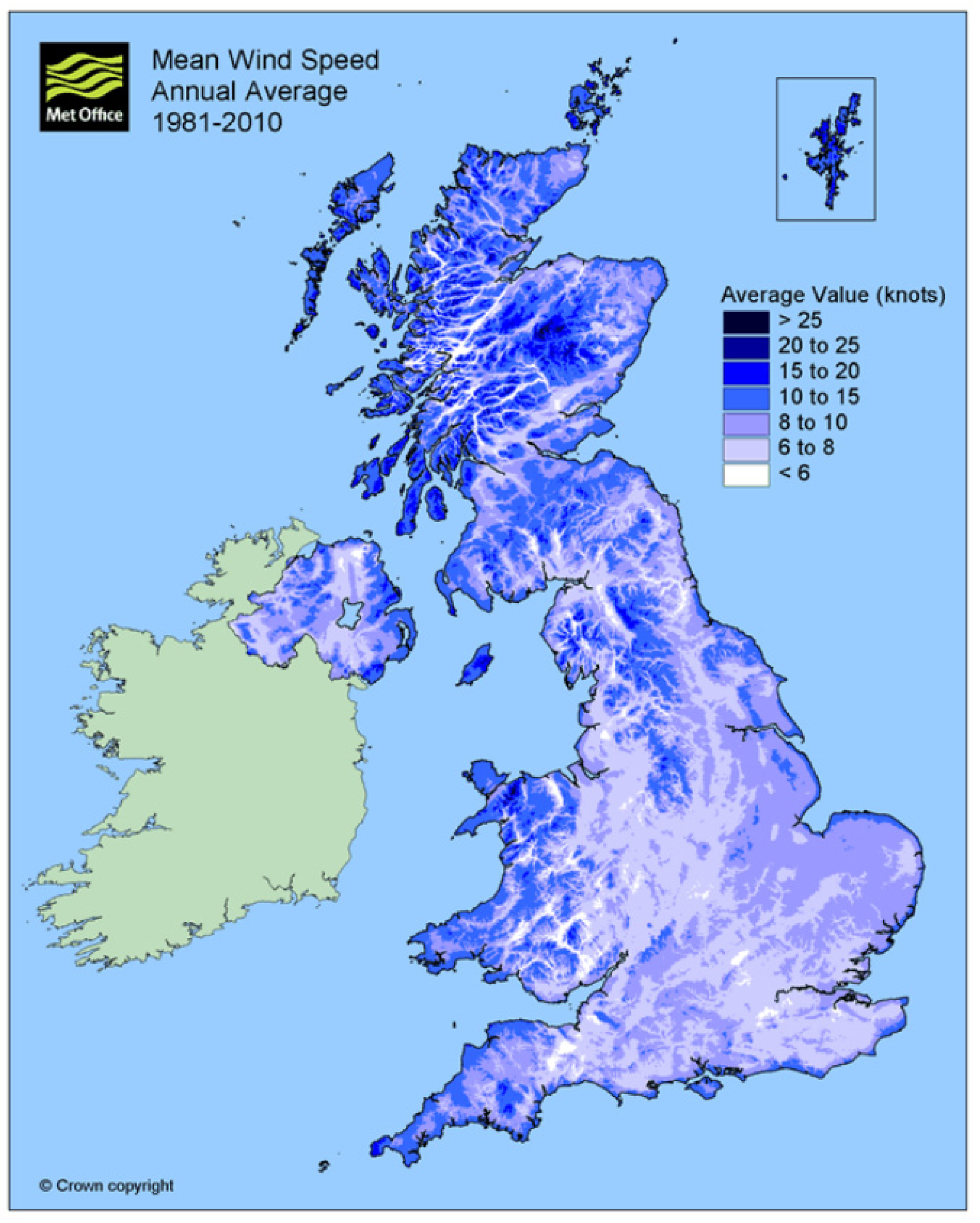
2.4.3. Wind Resource
Wind availability from within the UK territorial waters is a rich environment of potential energy, with “an estimate that over 80% of Europe’s wind energy passes over water deeper than 60 m” according to [
2]. This is supplemented with expected mean annual wind speeds of 9.75 m/s (around 19 knots) and greater according to [
18] analysis at a hub height of 80 m as shown in
Figure 1.
Scotland’s wind potential is shown in greater detail when the average wind speed is compared against NREL’s wind plant characteristic chart, seen in
Table 2, where it presents wind resource as the highest contributing factor in offshore wind turbine design and operations.
2.4.4. Net Capacity Factor
The maximum capacity of the wind turbine is theorized to be only able to capture 0.59% of the total kinetic energy of the wind. The Theory, better known as the Betz limit, stands true. Entailing associated losses can be attributed to turbine design or wind resource characteristics [
17], the net generational performance slips further when additional effects such as array wake losses, environmental aspects, transmission losses and blade soiling losses are accounted for [
17]. According to [
19], historical net capacity figures lie in the region of 28.5% to 49.5%. However, [
19] suggests that load factors for 13–15 MW turbines may reach as high 51–53%, depending on location.
Weaknesses associated with AEP calculation are the exclusion of degradation and downtime loss from maintenance and repair. Both NREL and BEIS do not account for either factor within both calculations.
Performance degradation from age affects all wind farms, no matter the generation of turbine. As such, any decrease in performance would raise the levelised cost of electricity. According to [
20] “wind turbines are found to lose 1.6 ± 0.2% of their output per year”, resulting in a net increase LCOE valuation of 9% over a 20-year period.
Currently the total number of expected days the turbine will be realistically operational is not factored into the BEIS LCOE calculation, thus the total generational capacity currently represents 8760 hours of operation every year for the expected service life of the turbine. An analysis by [
21] estimated the net availability from a Dutch offshore windfarm located 35 km of the coast ranged from 85% to 94% due to maintenance and repair.
Gathering accurate and certifiable data surrounding these factors is strenuous at best without the help of contracting offshore support companies. Using justifiable assumptions can mitigate this effect into a generalized net capacity factor. The net capacity factor will be used to adjust the nameplate capacity to the appropriate rate based on low, mid, and high scenarios.
A sensitivity analysis in Case Study B examines the extent the expected net capacity factor has upon the LCOE calculations across all three calculators: BEIS, Fixed and floating.
2.4.5. Discount Rate
Selection of an applicable discount rate to a subsidy free model bid for offshore wind is a highly speculative contentious area of financing. In LCOE literature, [
22] claims that the discount rate has a significant effect on LCOE valuations. Furthermore, [
23] points out that the BEIS hurdle rate has a direct “effect of raising the LCOE for technologies considered to be riskier, and potentially skews the metric in favour of apparently less risky technologies”. The potential skew in question, applies to the difference in technology expenditure profiles. With offshore wind dominated by high initial overnight costs in retrospect of Combined Cycle Gas Turbine (CCGT) plants with elongated fuel and operation costs. Current CfD contracts offer zero risk guarantees for the generator/owner of offshore windfarms with applied discount rates of 8.9% [
14]. Adopting a zero-bid subsidy model drastically increases the risk factor and subsequently the level of the discount rate. Identifying a suitable rate for zero subsidy models is explored further in Case Study C.
2.4.6. OPEX
The operational expenditure covers the expected cost from ongoing maintenance and repair of the windfarm. OPEX is particularly sensitive to distance and the accessibility of usable ports that afflict the duration of the planned activities. NREL LCOE accurately reflects OPEX costs by considering a multitude of factors using the Netherlands energy centre and research operation and maintenance tool [
17]. Comparatively, the BEIS metric using figures published in the underlying report for the Electricity Generation Costs, uses data that was collected from internal sources and five developers [
24]. As such different parameters are reflected in the LCOE OPEX calculations but have their own certifiable merit.
2.5. BEIS Deterministic Calculation
The data used for the LCOE BEIS calculation comes from Electricity Generation Costs central case scenario study for offshore round three, commissioning in 2025 [
14]. The calculated parameters used for the BEIS calculation is as tabulated in
Table 3.
When authors calculated the LCOE to that of the BEIS published value shown in
Table 4, there is a difference in LCOE valuations of 3% for the central case study. A very small but notable difference in value.
Furthermore, in supportive evidence of merit for the LCOE calculator design, Williams and Rubert [
23] produced a similar LCOE summation from a detailed EXCEL spreadsheet based upon a central case study for an offshore wind farm development in 2020. Comparative analysis between the two Excel spreadsheet results from
Table 4 and
Table 5 produced an LCOE evaluation difference of less than 1%, with only minor variations in parameter value selection. The parameter valuations used to calculate the LCOE tabulated in
Table 4 derive from the UK governments own LCOE Evaluation of offshore wind energy. It is concluded that LCOE valuations produced under the BEIS designed spreadsheet in this report are reliable to within a small degree of error.
2.6. BEIS Calculation Methodology
The BEIS methodology incorporates five potential levels of financing. Multiplication factors are applied to the central case study parameter data to represent possible cost reductions or increases.
Table 6 is a tabulation of the varying scenarios with the associated multiplication factors.
From the possible scenarios, there are five thousand and forty possible variations that can be applied to the BEIS LCOE calculator. Results presented in this paper are done across all scenario sets with all parameters set at the same multiplication factor.
Associated weaknesses have been identified in the spreadsheet process. Using such a small scenario of data limits the effectiveness of the produced LCOE result. However, the calculation design allows the potential of more multiplication factors and scenarios to be added to suit user requirements. Enabling the calculator to be useful in potential future studies in LCOE valuations.
The sensitivity a parameter has on the calculation is displayed as a percentage relative in aspect to the total capital or operational expenditure costs on the Excel spreadsheet.
2.7. Fixed and Floating Wind Farms Valuations
Data used for the fixed and floating offshore windfarm capital and operating expenditure, is drawn from the author’s interpretation of the published figures from the 2016 Cost of Wind Energy Review [
15], System Advisor Model (SAM) legacy version 2013 [
16] and Renewable Power Generation Costs in 2012: An Overview [
25].
Moné et al. [
26] concluded that the Fixed-Bottom Offshore Reference Project the expected turbine capital costs is 1660
$/kW. Equating that term to a European figure expected in 2012, provides a value of 1200 £/kW. This value is supported by International Renewable Energy Agency (IRENA) publishing the weighted average cost of the turbine at 1600
$/kW for 2010 [
26].
From the published percentage breakdowns of LCOE model evaluations by NREL, as shown in
Table 7 and
Table 8. A calculator was developed to replicate the NREL model performance. The turbine cost was extrapolated from the data to replicate the remainder of the CAPEX and OPEX expenditure values used in the remaining calculator models [
17].
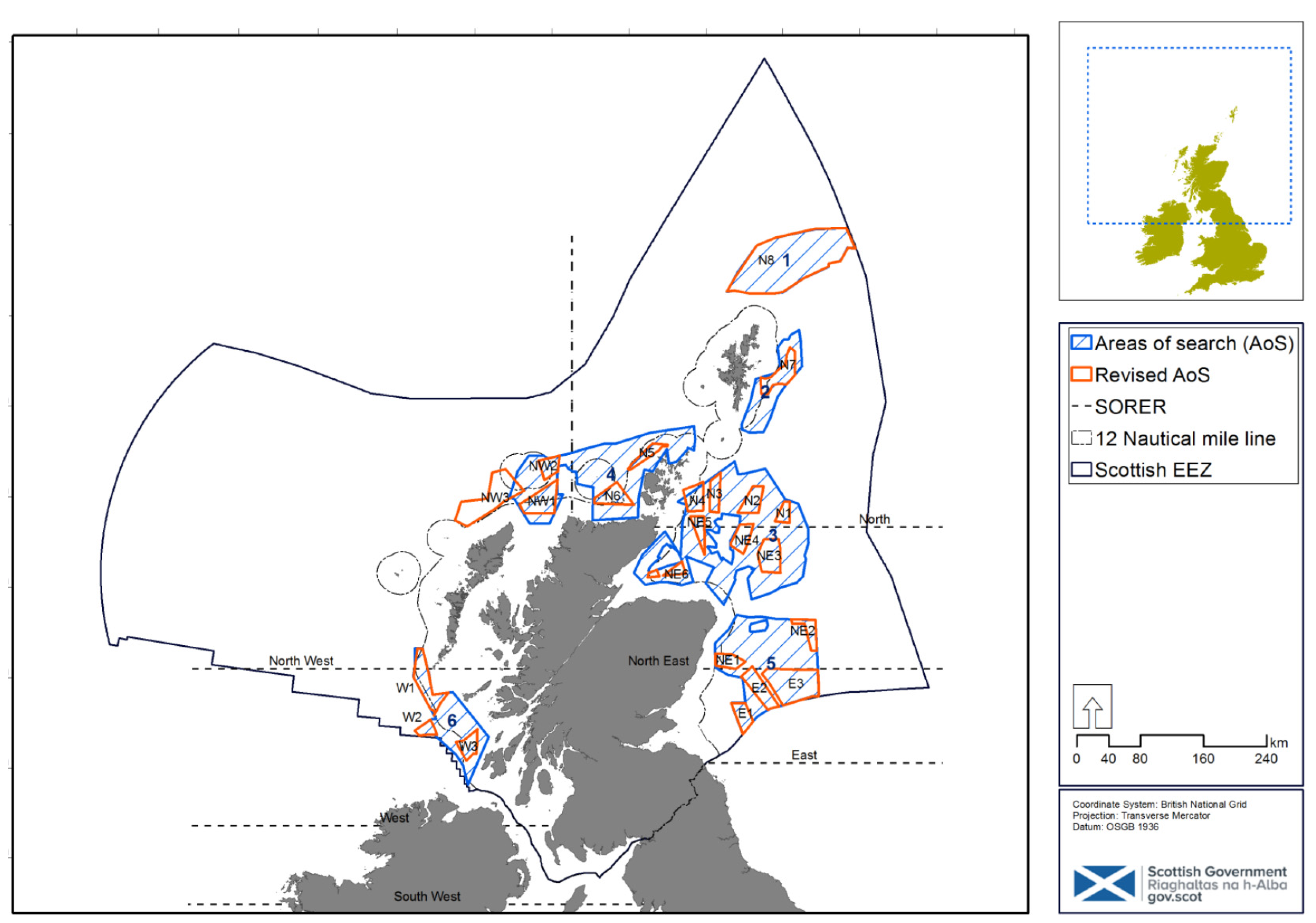
Applying the same scenario method to the floating and fixed calculators, there are over six billion possible combinations that can be applied to the calculators for all location parameters, areas, sites, turbine specifications. Rating and quantity are based on Scottish Exclusive Economic Zone from offshore Sectoral Marine Plan [
2] as illustrated in
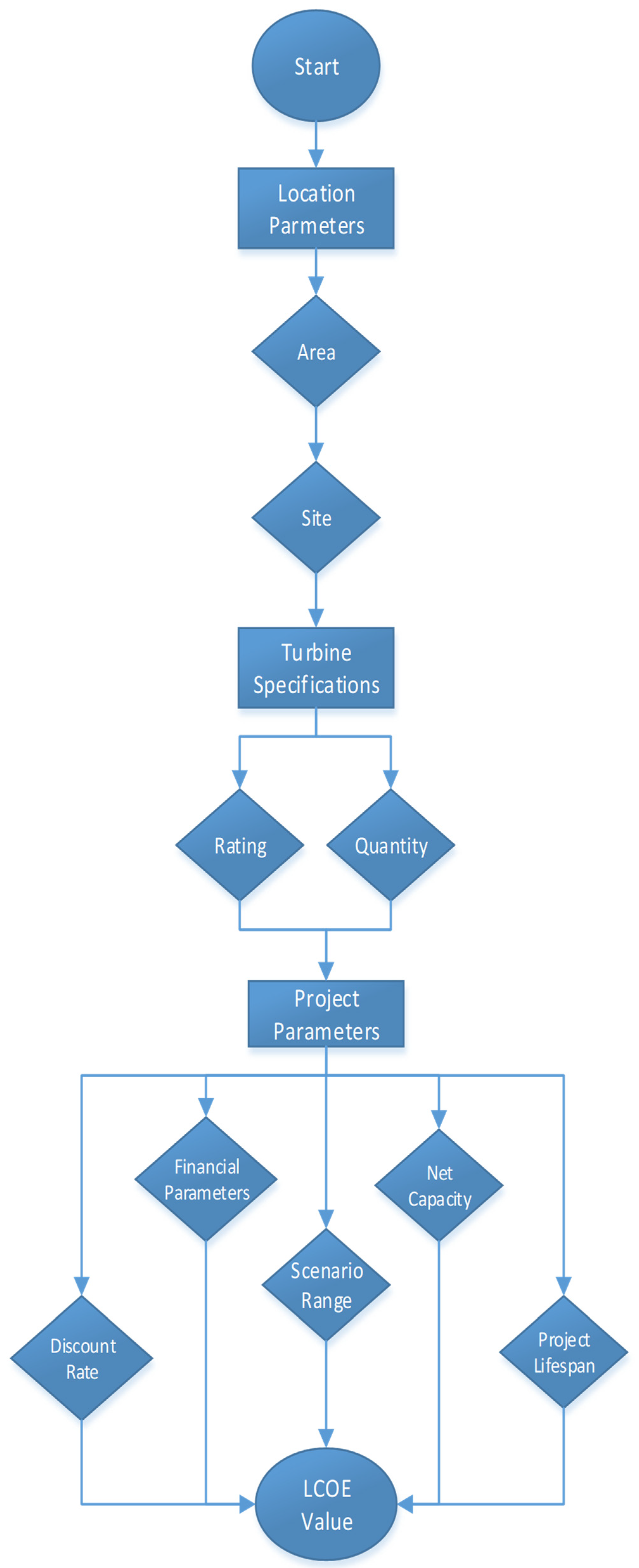
Figure 2 where it will be the basis for the first part of the flow chart as illustrated in
Figure 3.
Results presented in this paper are done across all scenarios sets with all parameters set at the same multiplication factor for simplicity. A flowchart detailing the sequential steps taking to produce an LCOE from the calculators can be seen in
Figure 3.
3. Results
Determining whether the zero-bid proposal has a realistic probability for a future inside the Scottish sectoral marine plan is emphasized in the following paper. A range of scenarios has been established that represent four following case studies. Case Study A: Effect of the total windfarm capacity against LCOE under the BEIS calculation methodology. The method will further illustrate the parameters required for an LCOE to reach a suitable value under aurora estimations for a net zero policy. Case Study B: Sensitivity analysis of net discount factor across all three calculators to determine a reputable figure of selection that is applicable to the zero subsidy models. Case Study C: Studies the levels of sensitivity the discount factor and net capacity factor has upon the LCOE valuations across all three calculators. This is resulting in idealized rates required across the distribution for a zero-bid policy. Case Study D: Analysis of the Dutch zero-subsidy models applied to the UK BEIS calculator. Removal of the applied connection and use of system charge are done to represent the government handling electrical connections.
3.1. Case Study A
3.1.1. Introduction
In the last ten years, the average offshore wind farm size has increased from 651 MW as of 2018 [
27]. Understanding the ensuing LCOE effects against expected capacities are integral for future developments in offshore wind.
3.1.2. Methodology
Generational capacity is measured from ranges ten to ten thousand using the BEIS calculator. A range of cost scenarios are applied to BEIS parameters to produce correlated LCOE values. This process is repeated for different operational lengths of twenty, fifteen and ten. The control variables used for this case study are as follow: discount rate is 8.9% and capacity factor is 48%.
3.1.3. Results
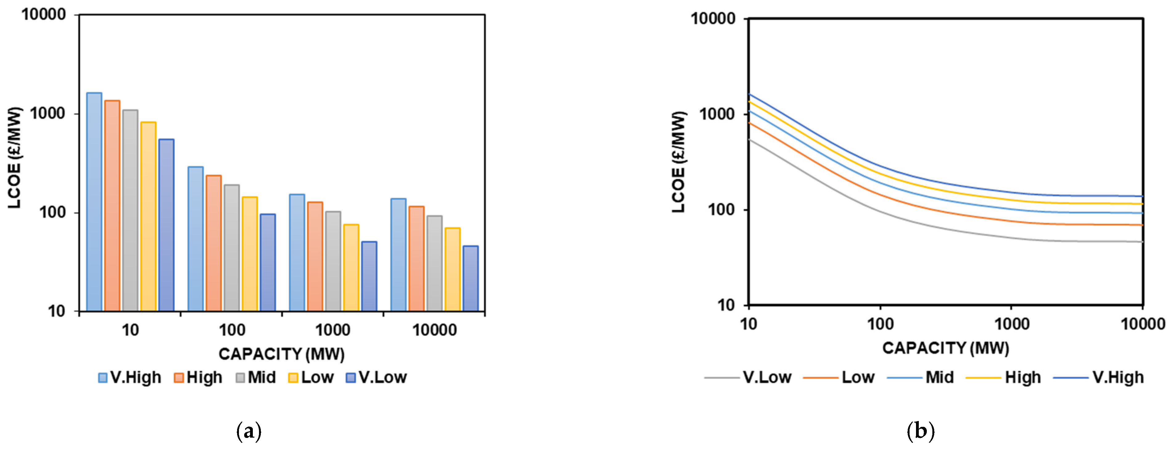
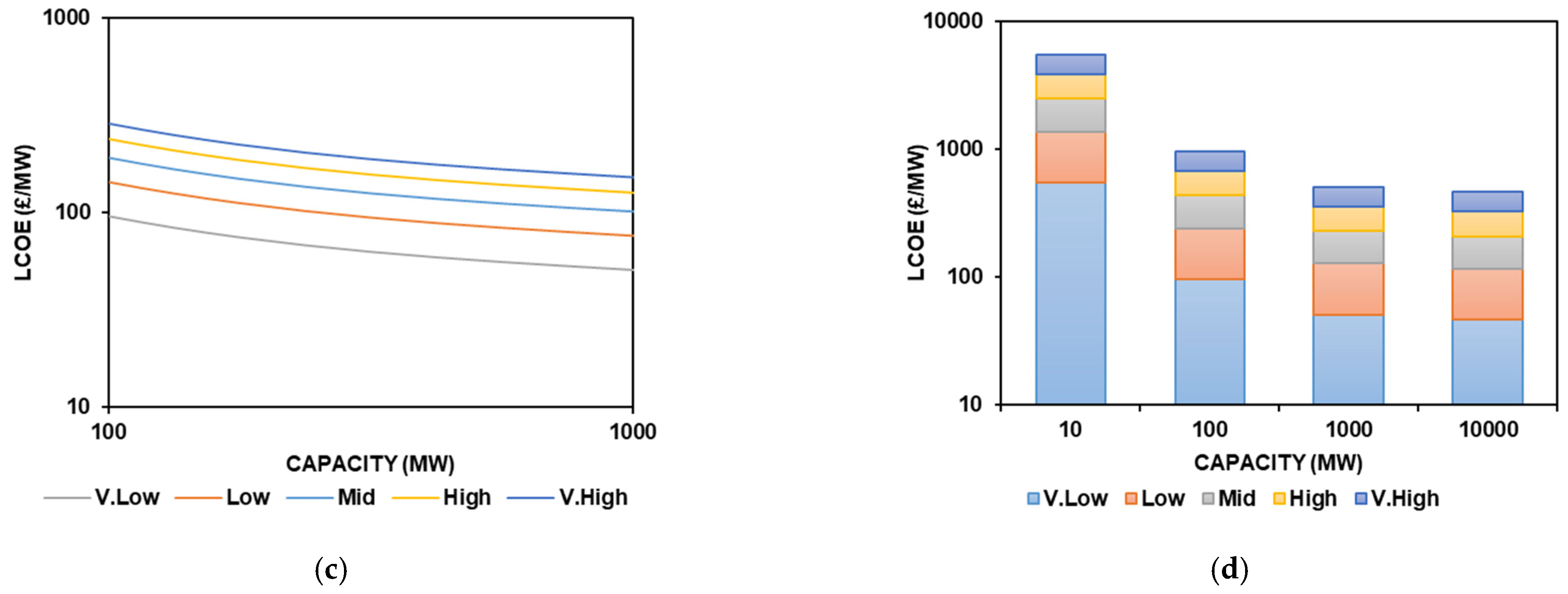
Figure 4a shows a 25-year distribution of the calculated LCOE values to the applied scenarios. The demographical curvatures can be seen in
Figure 4b with the following expanded emphasis on LCOE as shown in
Figure 4c.
Figure 4d illustrates the generational capacity LCOE ranges grouped into the correlated scenarios.
The total values for the LCOE’s at the given generational capacities with their correlated scenarios across the different operational years were calculated. The average LCOE depreciation per year from twenty-five years of operation is shown in
Table 9. This showcases the effect of removing a year of operational lifespan effects LCOE evaluations at an expected generational capacity.
From a logarithmic generational capacity scale, the LCOE drops at a considerate rate before starting to normalize at capacities over one hundred megawatts of capacity. Percentage depreciation from that point forward is approximately 4.7% per every added 100 MW. This drops further to less than 1% when considering over a thousand megawatts. The depreciation of LCOE is clearly visibly in
Figure 4c. The operational length of an offshore windfarm has a significant effect at low generational capacities as seen in
Table 9, which depreciates as the generational capacity is increased. After 1000 MW, the depreciation difference is almost stabilized.
3.2. Case Study B
3.2.1. Introduction
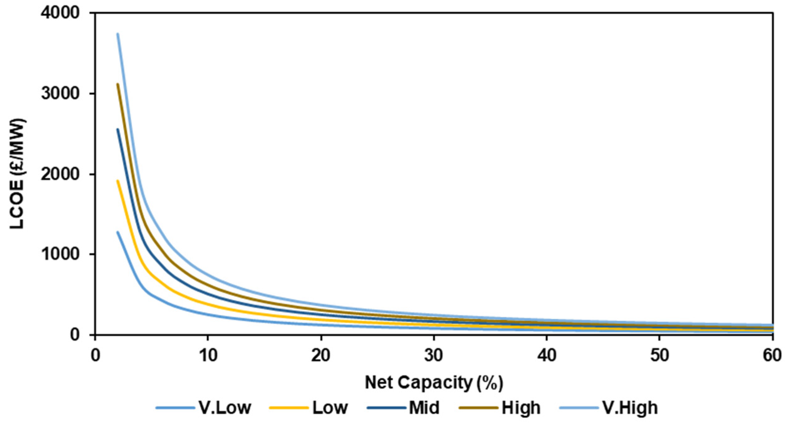
Larger and more powerful turbines coupled with technological advancements have raised the expected net capacity of the offshore windfarms. Case study B covers the extent to which the net capacity factor has effects on the possible outcome of pure and balance of system zero bid subsidy models.
3.2.2. Methodology
The range over which the net capacity is analysed from across all three calculator configurations are 0–60%. Control variables are the discount rate and the generational capacity, as shown in
Table 10.
3.2.3. Results
From the analysis, the only data of note that are applicable to pure and balance of system zero bid models are shown in
Table 11 and
Table 12. The data in these tables are colour dependent based on LCOE values.
Red donates a scenario at which a loss would occur
Green indicates a range at which a zero bid CfD is applicable
Blue highlights the LCOE when a pure subsidy free bid is valid
From the input parameters, under very-low-cost reduction, with high-capacity factors is a zero-subsidy model achievable in these circumstances. From the observation of data,
Figure 5 shows the output data for the BEIS calculator under variable cost scenarios over 25 years. The effect of the net capacity factor upon LCOE calculations have a minor effect on the outcome. In net capacity ranges of 10%, average LCOE adjustment per percentage change for a very low case scenario is shown below in
Table 13.
3.3. Case Study C
3.3.1. Introduction
One of the most speculative parameters for LCOE calculations is the applied discount rate. The discount rate reflects the pre-tax financing costs that are defined as the minimum project return that a plant owner would require over a project’s lifetime on a real pre-tax basis [
5]. Adjustment of the discount rate is highly notional. The greater risk associated with a planned development will subsequently increase the associated discount rate that operators are expected to pay to secure financial assets while trying to maintain feasible equality returns.
3.3.2. Methodology
Applying a range of discount rates against possible case scenarios for all three calculators will illustrate the potential discount rates that are necessary to implement pure subsidy and a balance of system model scheme.
3.3.3. Results
From the subsequent LCOE calculations under the five scenario methods, a viable range of the minimum expected threshold of generation is identified in
Table 14,
Table 15,
Table 16,
Table 17,
Table 18 and
Table 19 that meets auroras expected threshold values for the project to break even for a net zero and pure subsidy scheme. If it does not meet the minimum threshold, it will be considered as not applicable (N/A) in the Tables.
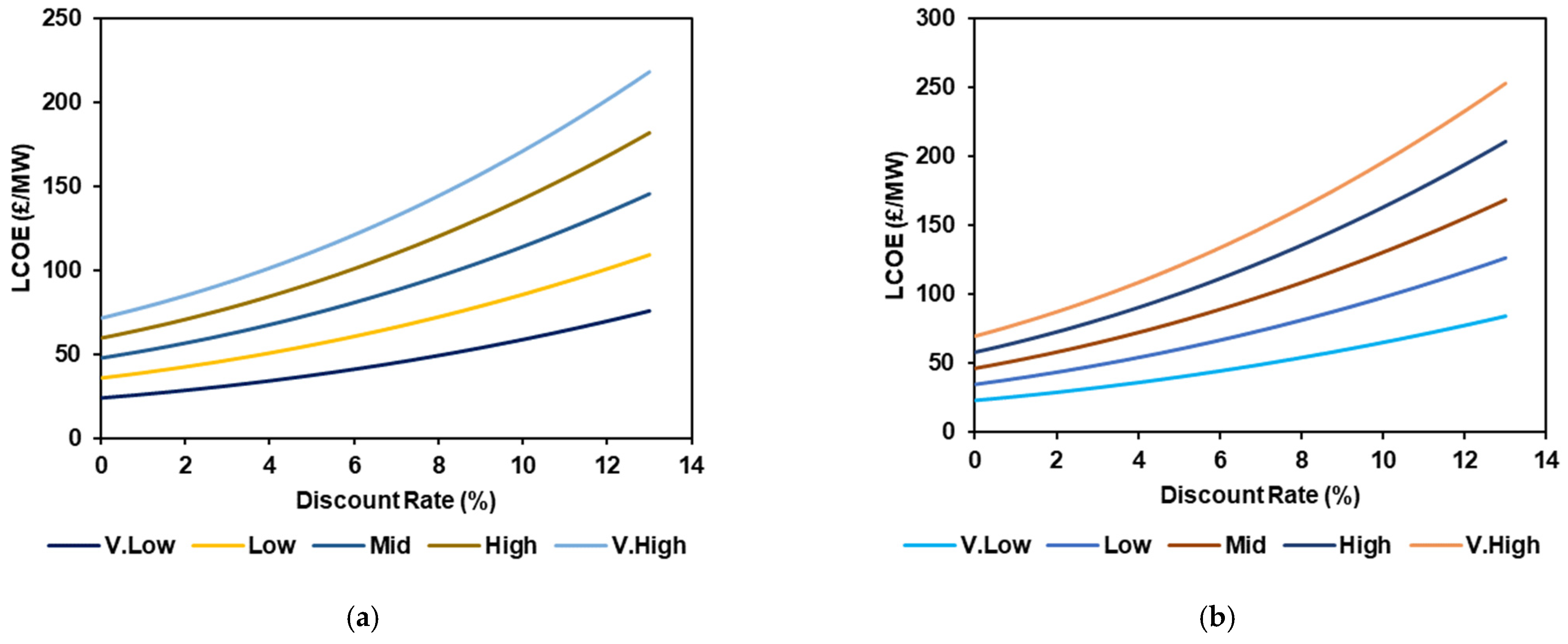
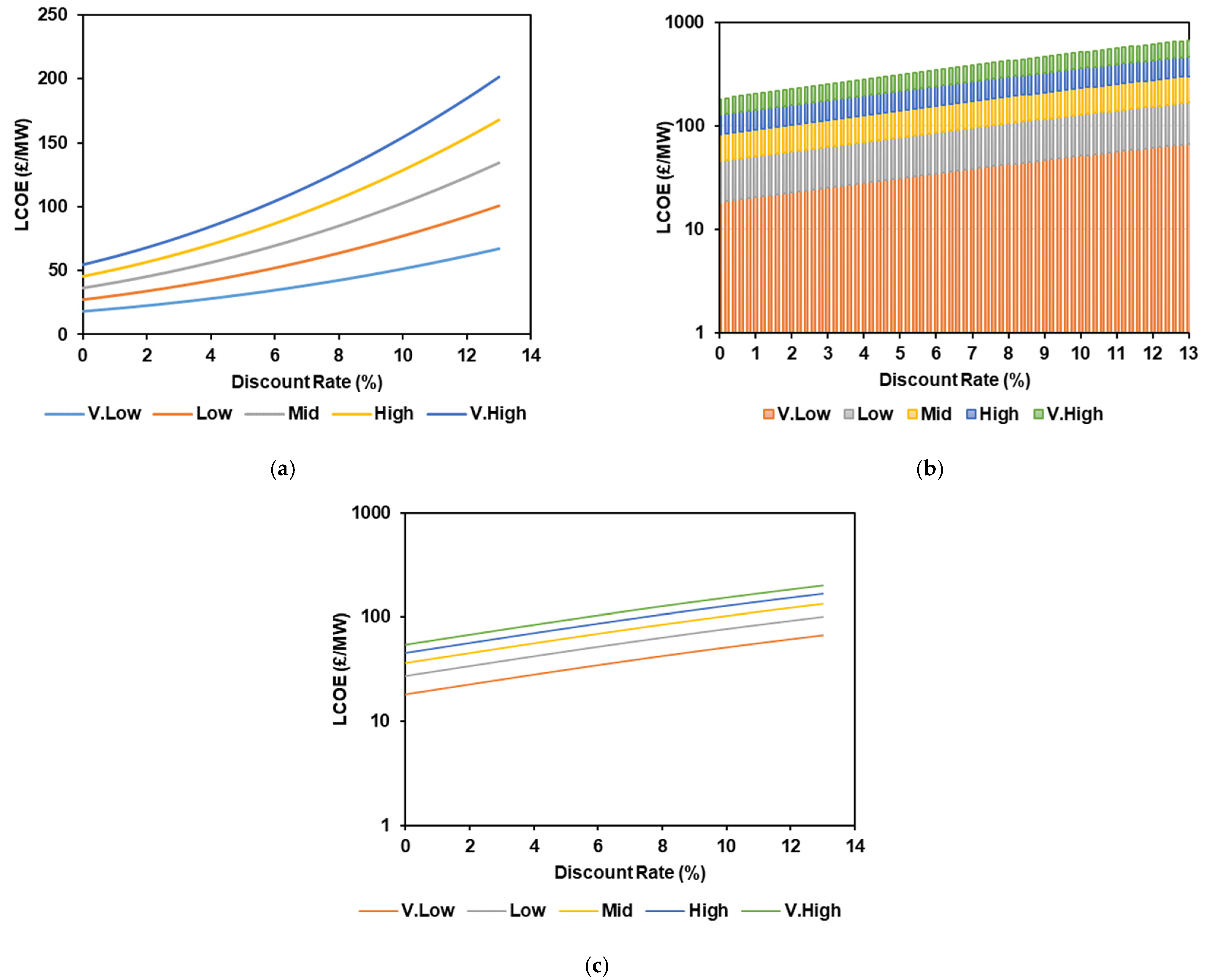
Figure 6a–c illustrate the direct correlation demographic between the LCOE and discount rate for all three calculators. The LCOE figure increases at a higher rate as the discount rate rises. Only under low favourable financing conditions can a reasonable LCOE value (>100 £/MW) be achieved with a discount rate of (8.9%).
3.4. Case Study D
3.4.1. Introduction
An analysis of the Dutch subsidy model involves testing the feasibility of integrating the Dutch and Scottish government policies. Integration of the Dutch zero subsidy model requires the adoption of two main legislative pieces: The Offshore Wind Energy Act, introduced in 2015 and the Offshore Grid Act, effective 2016 [
28]. Under the acts, the Dutch “government is responsible for choosing a location for the proposed plant and assure that construction and operation of the plant is aligned with all governmental institutions and that it will receive grid connection” [
29]. Implementation of these policies has seen a commitment from the industry to implement a cost-saving strategy in the hopes of reducing expected construction and operational expenditure of offshore windfarms by 40% by 2020 [
19].
Replicating the scenario for the Scottish government will require new or adapted acts from the Dutch legislative pieces to be adopted into the Sectoral Marine plan and the Scottish Energy Target.
3.4.2. Methodology
To represent the Dutch model policy change, the BEIS calculation has been carried out by removing the operational expenditure denoted by the Connection and Use of System Charges costs from the BEIS LCOE calculator. Under the circumstances, the National Grid will shoulder all responsibility for the handling of the grid connection to the offshore windfarm.
3.4.3. Results
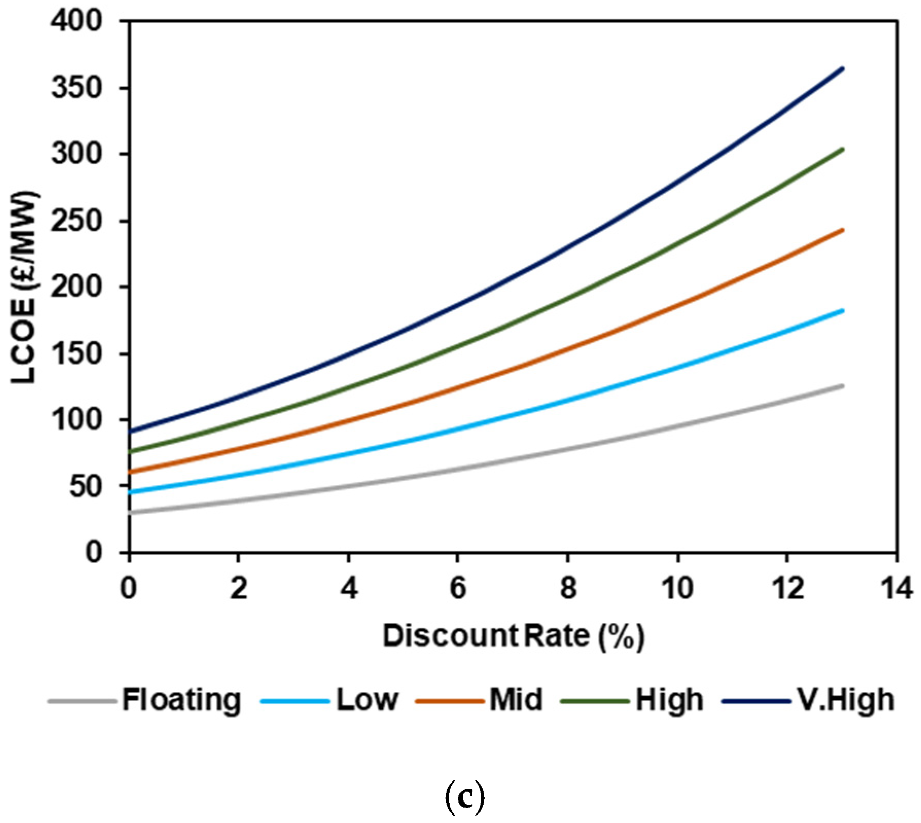
The LCOE demographic against discount rate when the connection and system charge is disregarded is shown in
Figure 7. In comparison to previous LCOE
Figure 6 in case study C, the discount rate has a modest impact decline on the reduction of LCOE values.
The identified cases in which the discount rate becomes applicable to generate at a neutral or profit LCOE is shown in
Table 20 and
Table 21.
4. Discussion
From the data produced in Case Study A, it is recommended that an offshore windfarm size should reach between 600–1000 MW of generational capacity. With emphasis placed on reaching the upper amount. At this point LCOE depreciation is minimal, even across all financial scenarios. Thus, providing an optimal scenario at which LCOE fluctuations are negligible.
From
Table 11 and
Table 12 in Case Study B, it is evident the greater the net capacity factor, the lower the correlated LCOE value. Current LCOE predictions using 48% net capacity factors reflect that a low sensitivity range is realistic. It is obligatory to recommend offshore turbines with the most efficient net factors are implemented where possible. High net capacity factors are imperative towards LCOE values for subsidy free models as shown in
Figure 5. Caution is advised however, as degradation is not accounted for.
Table 13 illustrates the possible LCOE drop per percentage variation. This can significantly affect subsidy free models in the long term.
From the data procured in Case Study C, cost predictions/reductions for financial parameters are substantial for delivering a suitable discount rate. Under the low scenario, a discount rate reduction of almost 60% or less is required from a standard hurdle rate of 8.9% for a subsidy model to become viable. Furthermore, the range at which the net zero bid is suitable is very narrow. It is recommended the fixed discount rate be variable to each theoretical windfarm to more accurately reflect site-specific financial conditions.
With reference to Case Study D, removing the Connection and Use of System Charges has a significant effect on the LCOE valuations. Almost 50% of the OPEX is covered by these charges. This has increased the expected discount rate by approximately two percent across all scenarios as seen above in
Table 20 and
Table 21. Thus, making the LCOE less susceptible to the assumed financial parameters. A discount rate of around 5% is applicable to a realistic expectation of a 25% drop in financial costs.
As a result of all the case studies conducted, key focal points have been identified that are significant for the development of subsidy free offshore windfarms to become a reality in future, including:
Increase CfD contract operational length to thirty years.
Enable offshore wind access to capacitive and ancillary services and markets.
Introduction of larger and more powerful turbines to be implemented to alleviate CAPEX expenditure
Significant cost reductions of greater than 25%, are to be expected for the future online developments post 2025.
Reduction in the expected discount rate below 8%.
Energy wholesale market prices are expected to increase at a higher rate than Europe.
Cost of carbon floor price is to increase. Only close to shore fixed turbines are economically viable for a net zero CfD.
5. Conclusions
Application of the LCOE metric is always regarded as an assumption. Yet, the use of LCOE is widespread, with numerous iterations occurring. This investigation has found a range of scenarios at which zero subsidy bids are applicable under the CfD policy.
From Case Study A, it is recommended a proposed windfarm have operational capacity ranging between 600–1000 MW as shown in
Figure 4b. Thus, significantly reducing any LCOE evaluation. Any further increase in generational capacity will produce diminishing returns.
When selecting a turbine for a proposed windfarm, it is recommended from Case Study B that turbines with a minimum rated capacity factor of 40% be selected. Turbine degradation at this range will only produce a marginal LCOE depreciation as shown in
Table 1 on a yearly basis.
In Case Study C, it is concluded that there is a direct correlation between discount rate and the CAPEX cost as shown in
Figure 5. The LCOE figure is more significant the greater the discount rate. In context, the only identifiable regions at which a reasonable level of discount rate occurs is at very low-cost expectations.
From the investigation of subsidy free bids for offshore windfarms, it is recommended that, where economically viable, a net zero CfD balance of system scheme be implemented by the UK government. A net zero CfD will provide an upsurge in expansion for offshore wind over current CfD agreements. The consequent reduction in auction price bid price would free up additional funding for other windfarms under the sectoral marine plan that are not applicable to a subsidy free model. Moreover, ultimately reducing consumer costs and carbon emissions.
However, a net zero CfD is limited. A significant reduction in cost is necessary, high net turbine capacity factors are required. Additionally, policies such as revenue stabilization and access to alternative revenue streams are required in correlation with expected cost reductions to help lower the appreciable discount rate. Nevertheless, the generator/owner will still be provided with a guaranteed source of revenue that should assist in mitigating some of the added risk.
Further work to be carried out that can reinforce the zero-subsidy model application, include:
Brexit analysis on cost services and government policy changes.
Integrating the Monte–Carlo method to provide the likelihood of each subsidy model occurring within a defined set of parameters.
Find detailed financial parameters to support more accurate LCOE evaluation.
Detailed analysis of policy integration required.
Operator/owner survey of possible scenario outcomes for future developments.
The authors express caution when taking values produced in this paper, hence, the analysis of zero bid proposal and LCOE assumptions are speculative and are based upon the authors’ analyses.
Author Contributions
Conceptualization, C.S. and A.S.A.; methodology, C.S. and A.S.A.; software, C.S.; validation, F.M.-S. and A.S.A.; formal analysis, C.S.; investigation, C.S.; resources, C.S. and A.S.A.; data curation, C.S. and F.M.-S.; writing—original draft preparation, C.S.; writing—review and editing, C.S., F.M.-S., M.A., J.A.A.-R., A.S.A., M.F.M.S., M.K.R., M.N.M. and M.Z.; visualization, C.S. and F.M.-S.; supervision, A.S.A. and M.K.R.; project administration, F.M.-S. and A.S.A.; funding acquisition, F.M.-S., A.S.A., J.A.A.-R., M.N.M. and M.Z. All authors have read and agreed to the published version of the manuscript.
Funding
F.M.-S. acknowledged the contribution from Edinburgh Napier University through Starter Research and Innovation Grants (Reference No REG2021/22). M.N.M. acknowledged the support from Ministry of Higher Education Malaysia under Fundamental Research Grant Scheme (R.K130000.7856.5F406). M.Z. appreciated the support from Universiti Tun Hussein Onn Malaysia under TIER 1 (Vot H930). The Article Processing Charges (APC) are funded by the National Research and Development Agency (ANID) through the projects Fondecyt regular 1200055 and Fondef ID19I10165.
Institutional Review Board Statement
Not applicable.
Informed Consent Statement
Not applicable.
Data Availability Statement
Not applicable.
Conflicts of Interest
The authors declare no conflict of interest. The funders had no role in the design of the study; in the collection, analyses, or interpretation of data; in the writing of the manuscript, or in the decision to publish the results.
References
- Scottish Government. Scottish Energy Strategy: The Future of Energy in Scotland; The Scottish Government: Edinburgh, UK, 2017.
- Marine Scotland Science. Scoping ‘Areas of Search’ Study for offshore wind energy in Scottish Waters, 2018; The Scottish Government: Edinburgh, UK, 2018.
- GWEC. Global Wind Energy Report: Annual Market Update 2017; GWEC: Brussels, Belgium, 2018. [Google Scholar]
- Welch, J.B.; Venkateswaran, A. The dual sustainability of wind energy. Renew. Sustain. Energy Rev. 2009, 13, 1121–1126. [Google Scholar] [CrossRef]
- Bang, G.; Lahn, B. From oil as welfare to oil as risk? Norwegian petroleum resource governance and climate policy. Clim. Policy 2020, 20, 997–1009. [Google Scholar] [CrossRef]
- Ortega-Izquierdo, M.; del Río, P. An analysis of the socioeconomic and environmental benefits of wind energy deployment in Europe. Renew. Energy 2020, 160, 1067–1080. [Google Scholar] [CrossRef]
- Gielen, D.; Boshell, F.; Saygin, D.; Bazilian, M.D.; Wagner, N.; Gorini, R. The role of renewable energy in the global energy transformation. Energy Strategy Rev. 2019, 24, 38–50. [Google Scholar] [CrossRef]
- Enevoldsen, P.; Permien, F.H.; Bakhtaoui, I.; von Krauland, A.K.; Jacobson, M.Z.; Xydis, G.; Sovacool, B.K.; Valentine, S.V.; Luecht, D.; Oxley, G. How much wind power potential does Europe have? Examining European wind power potential with an enhanced socio-technical atlas. Energy Policy 2019, 132, 1092–1100. [Google Scholar] [CrossRef]
- Sawant, M.; Thakare, S.; Rao, A.P.; Feijóo-Lorenzo, A.E.; Bokde, N.D. A review on state-of-the-art reviews in wind turbine-and wind-farm-related topics. Energies 2021, 14, 2041. [Google Scholar] [CrossRef]
- Spyridonidou, S.; Vagiona, D.G. Systematic review of site-selection processes in onshore and offshore wind energy research. Energies 2020, 13, 5906. [Google Scholar] [CrossRef]
- Herbert-Acero, J.F.; Probst, O.; Réthoré, P.E.; Larsen, G.C.; Castillo-Villar, K.K. A review of methodological approaches for the design and optimization of wind farms. Energies 2014, 7, 6930–7016. [Google Scholar] [CrossRef]
- Probst, O.; Cárdenas, D. State of the art and trends in wind resource assessment. Energies 2010, 3, 1087–1141. [Google Scholar] [CrossRef] [Green Version]
- Mott MacDonald. UK Electricity Generation Costs Update; Mott MacDonald: Brighton, UK, 2010. [Google Scholar]
- DECC. Contracts for Difference: Consultation on Changes to the CFD; DECC: London, UK, 2016.
- Stehly, T.; Heimiller, D.; Scott, G. 2016 Cost of Wind Energy Review; National Renewable Energy Laboratory (NREL): Alexandria, VA, USA, 2017.
- Cartelle Barros, J.J.; Lara Coira, M.; de la Cruz López, M.P.; del Caño Gochi, A. Probabilistic life-cycle cost analysis for renewable and non-renewable power plants. Energy 2016, 112, 774–787. [Google Scholar] [CrossRef]
- Moné, C.; Hand, M.; Bolinger, M.; Rand, J.; Heimiller, D.; Ho, J. 2015 Cost of Wind Energy Review; National Renewable Energy Laboratory (NREL): Alexandria, VA, USA, 2017.
- Met. Office. Where Are the Windiest Parts of the UK? Available online: https://www.metoffice.gov.uk/weather/learn-about/weather/types-of-weather/wind/windiest-place-in-uk (accessed on 15 March 2022).
- Aurora Energy Research Ltd. The New Economics of Offshore Wind; Aurora Energy Research Ltd.: Oxford, UK, 2018. [Google Scholar]
- Staffell, I.; Green, R. How does wind farm performance decline with age? Renew. Energy 2014, 66, 775–786. [Google Scholar] [CrossRef] [Green Version]
- Van Bussel, G.J.W.; Zaaijer, M.B. DOWEC concepts study, reliability, availability and maintenance aspects. In Proceedings of the 2001 European Wind Energy Conference and Exhibition, Copenhagen, Denmark, 2–6 July 2001; Volume 113, pp. 557–560. [Google Scholar]
- Manzhos, S. On the choice of the discount rate and the role of financial variables and physical parameters in estimating the levelized cost of energy. Int. J. Financ. Stud. 2013, 1, 54–61. [Google Scholar] [CrossRef] [Green Version]
- Aldersey-Williams, J.; Rubert, T. Levelised cost of energy—A theoretical justification and critical assessment. Energy Policy 2019, 124, 169–179. [Google Scholar] [CrossRef]
- Ove Arup & Partners Ltd. Review of Renewable Electricity Generation Cost and Technical Assumptions: Study Report; Ove Arup & Partners Ltd.: London, UK, 2016. [Google Scholar]
- IRENA. Renewable Power Generation Costs in 2012: An Overview; IRENA: Abu Dhabi, United Arab Emirates, 2013. [Google Scholar]
- Moné, C.; Smith, A.; Maples, B.; Hand, M. 2013 Cost of Wind Energy Review; National Renewable Energy Laboratory (NREL): Alexandria, VA, USA, 2015.
- Wind Europe. Wind Energy in Europe in 2018: Trends and Statistics; Wind Europe: Brussels, Belgium, 2019. [Google Scholar]
- Böttcher, J. Rechtliche Rahmenbedingungen von EE-Projekten. Band 2, 1st ed.; BWV Berliner Wissenschafts-Verlag: Berlin, Germany, 2018; ISBN 978-3-8305-2982-8. [Google Scholar]
- IEA. Netherlands Offshore Wind Energy Act (Wet Wind op Zee); International Energy Agency: Paris, France, 2016. [Google Scholar]
Figure 1.
Scotland’s mean annual wind speed [
18].
Figure 1.
Scotland’s mean annual wind speed [
18].
Figure 2.
Wind Development Sites [
2].
Figure 2.
Wind Development Sites [
2].
Figure 3.
Flowchart description of calculator design.
Figure 3.
Flowchart description of calculator design.
Figure 4.
(a) 25 Year Case Scenarios; (b) Scenario distribution; (c) Enhanced distribution; and (d) Generational capacity.
Figure 4.
(a) 25 Year Case Scenarios; (b) Scenario distribution; (c) Enhanced distribution; and (d) Generational capacity.
Figure 5.
Net Capacity Factor vs. LCOE.
Figure 5.
Net Capacity Factor vs. LCOE.
Figure 6.
25 Year analysis for (a) BEIS LCOE; (b) Fixed LCOE, and (c) Floating LCOE.
Figure 6.
25 Year analysis for (a) BEIS LCOE; (b) Fixed LCOE, and (c) Floating LCOE.
Figure 7.
(a) 25-year scenario vs. discount rate; (b) 25-year range, and (c) Year sensitivity (LCOE difference of 15–25 year).
Figure 7.
(a) 25-year scenario vs. discount rate; (b) 25-year range, and (c) Year sensitivity (LCOE difference of 15–25 year).
Table 1.
BEIS’s LCOE Parameters.
Table 1.
BEIS’s LCOE Parameters.
| CAPEX | OPEX | Expected Generation |
|---|
Pre-developed costs Construction costs
Infrastructure | Fixed * OPEX
Variable * OPEX
Insurance
Connection costs
Carbon transport and storage costs
Decommissioning fund costs
Heat revenues
Fuel prices
Carbon costs expected | Capacity of plant
Expected availability
Expected efficiency
Expected load factor (all assumed baseload) |
Table 2.
BEIS Pure LCOE [
17].
Table 2.
BEIS Pure LCOE [
17].
| | Wind Plant Characteristics Associated with
Average Wind Speed |
|---|
| Average Annual Wind Speed at 80 m Hub Height (m/s) | ≤5.5 | 7.40 | 8.0 | 8.4 | ≥10.0 |
| Specific Power (W/m2) | 200 | 237 | 245 | 255 | 325 |
| Machine Rating (MW) | 2 | 2 | 2 | 2 | 2 |
| Rotor Diameter (m) | 113 | 104 | 102.0 | 100 | 89 |
| Hub Height (m) | 80 | 80 | 80 | 80 | 80 |
| CAPEX (£/kW) | 1.303 | 1.242 | 1.232 | 1.219 | 1.156 |
| OPEX (£/kW/year) | 38.3 | 38.3 | 38.3 | 38.3 | 38.3 |
| Capacity Factor * | 27% | 39% | 43% | 45% | 49% |
| FCR (real) [Real WACC ‡ = 5.7%] | 9.6% | 9.6% | 9.6% | 9.6% | 9.6% |
| LCOE (£/MWh) | 69.9 | 45.8 | 41.3 | 39.8 | 35.3 |
Table 3.
Parameter calculations according to government scenario.
Table 3.
Parameter calculations according to government scenario.
| Windfarm Parameter | Value |
|---|
| Nameplate General Capacity (MW) | 844 |
| Net Capacity Factor (%) | 48 |
| Discount Rate (%) | 8.9 |
| Pre-development period (£/kW) | 120 |
| Construction (£/kW) | 2100 |
| Infrastructure (£’000 s) | 323,000 |
| Insurance (£/MW/year) | 45,400 |
| Connection and Use of System | 47,000 |
| Charges (£/MW/year) | 3100 |
| Operational Years (years) | 25 |
| LCOE (£/MWh) | 103.32 |
Table 4.
Government LCOE Valuations.
Table 4.
Government LCOE Valuations.
| | Nuclear PWR-FOAK | COAL-ASC with Oxy Comb, CCS-FOAK | CCGT with Post CCS-FOAK | Coal-IGCC with CCS-FOAK | CCGT H Class | OCGT 600 MW
(500 h) | Offshore R3 |
|---|
| High CAPEX | 123 | 158 | 123 | 171 | 83 | 198 | 113 |
| Central | 95 | 136 | 110 | 148 | 82 | 189 | 100 |
| Low CAPEX | 85 | 125 | 102 | 137 | 80 | 182 | 88 |
| High CAPEX, high fuel | 124 | 169 | 132 | 183 | 90 | 209 | |
| Low CAPEX, low fuel | 84 | 120 | 85 | 132 | 66 | 160 | |
Table 5.
Parameter Calculation according to Williams and Rubert [
23].
Table 5.
Parameter Calculation according to Williams and Rubert [
23].
| Input Parameter | CCGT | Unmodified Wind Farm | Scaled Wind Farm |
|---|
| Capacity (MW) | 1200 | 844 | 844 |
| Availability/Capacity Factor (%) | 93 | 48 | 48 |
| Prebuild Costs (£/kW) | 10 | 120 | 74 |
| Construction (£/kW) | 500 | 2300 | 1409 |
| Infrastructure (£’000 s) | 15,100 | 323,000 | 197,870 |
| Fixed O and M (£/MW/year) | 12,200 | 47,300 | 28,976 |
| Variable O and M (£/MWh/year) | 3 | 3 | 2 |
| Fuel Cost Conversion Factor (%) (Converts fuel cost (p/therm) to annual variable cost (£/MWh)) | 110 | Zero Fuel Cost | Zero Fuel Costs |
| Insurance (£/MW/year) | 21,000 | 3300 | 2022 |
| Connection Charges (£/MW/year) | 3300 | 48,900 | 29,956 |
| Discount Rate (%) | 7.8 | 8.9 | 8.9 |
| Operating Life (years) | 25 | 25 | 25 |
| LCOE (£/MWh) | 47.00 | 103.88 | 58.50 |
Table 6.
Financial Scenarios.
Table 6.
Financial Scenarios.
| Scenario | Multiplication Factor |
|---|
| Very Low | 0.50 |
| Low | 0.75 |
| Mid | 1.00 |
| High | 1.25 |
| Very High | 1.50 |
Table 7.
Fixed and Floating Parameter Valuations [
17].
Table 7.
Fixed and Floating Parameter Valuations [
17].
| Parameter | Fixed | Floating |
|---|
| Turbine (£/kW) | 1200.00 | 1200.00 |
| Development (£/kW) | 51.06 | 54.30 |
| Engineering and Management (£/kW) | 58.36 | 119.46 |
| Substructure and Foundation (£/kW) | 503.34 | 1965.61 |
| Site Access, Staging and Port (£/kW) | 18.24 | 32.58 |
| Electrical Infrastructure (£/kW) | 328.27 | 570.14 |
| Assembly and Installation (£/kW) | 693.01 | 602.71 |
| Plant Commissioning (£/kW) | 29.18 | 43.44 |
| Insurance (£/kW) | 36.47 | 54.30 |
| Decommissioning (£/kW) | 178.72 | 65.16 |
| Contingency (£/kW) | 317.33 | 347.51 |
| Finance (£/kW) | 233.43 | 380.09 |
| OPEX (£/kW) | 50 | 38.4 |
| Nameplate Capacity (MW) | 800 | 800 |
| Net Capacity Factor (%) | 48 | 48 |
| Operational Years (years) | 25 | 25 |
| Discount Rate (%) | 8.9 | 8.9 |
Table 8.
Fixed and Floating Parameter Valuations [
17].
Table 8.
Fixed and Floating Parameter Valuations [
17].
| | Fixed—Bottom Substructure (£/kW/Year) | Fixed—Bottom Substructure (£/kWh) | Floating Substructure (£/kW/Year) | Floating Substructure (£/kWh) |
|---|
| Operation | 23.3 | 6.39 | 23.3 | 6.4 |
| Maintenance | 95.4 | 26.1 | 46.6 | 12.8 |
| OPEX | 118.7 | 32.5 | 69.9 | 19.2 |
Table 9.
LCOE Increase per Year.
Table 9.
LCOE Increase per Year.
| Scenario/Capacity (MW) | 10 | 100 | 1000 | 10,000 |
|---|
| V Low | 11.86 | 1.87 | 0.87 | 0.77 |
| Low | 17.79 | 2.81 | 1.31 | 1.16 |
| Mid | 23.72 | 3.74 | 1.74 | 1.54 |
| High | 29.65 | 4.68 | 2.18 | 1.93 |
| V High | 35.58 | 5.61 | 2.61 | 2.31 |
Table 10.
Control Parameters.
Table 10.
Control Parameters.
| Parameter | Windfarm |
|---|
| Nameplate Generational Capacity (MW) | 800 |
| Net Capacity Factor (%) | 0–60 |
| Discount Rate (%) | 8.9 |
Table 11.
Net Capacity (25 Years).
Table 11.
Net Capacity (25 Years).
| 25 Years | V. Low |
|---|
| Capacity Factor (%) | BEIS | Fixed | Floating |
|---|
| 46 | 55.598 | 61.688 | 89.320 |
| 48 | 53.282 | 59.117 | 85.599 |
| 50 | 51.151 | 56.753 | 82.175 |
| 52 | 49.183 | 54.570 | 79.014 |
| 54 | 47.362 | 52.549 | 76.088 |
| 56 | 45.670 | 50.672 | 73.370 |
| 58 | 44.095 | 48.925 | 70.840 |
| 60 | 42.626 | 47.294 | 68.479 |
Table 12.
Net Capacity (20 Years).
Table 12.
Net Capacity (20 Years).
| 20 Years | V. Low |
|---|
| Capacity Factor (%) | BEIS | Capacity Factor (%) | BEIS |
|---|
| 46 | 58.971 | 65.965 | 95.838 |
| 48 | 56.514 | 53.216 | 91.845 |
| 50 | 54.253 | 60.687 | 88.171 |
| 52 | 52.167 | 58.353 | 84.780 |
| 54 | 50.234 | 56.192 | 81.640 |
| 56 | 48.440 | 54.185 | 78.724 |
| 58 | 46.770 | 52.317 | 76.010 |
| 60 | 45.211 | 50.573 | 73.476 |
Table 13.
LCOE Sensitivity.
Table 13.
LCOE Sensitivity.
| Capacity Factor Range (%) | LCOE Sensitivity (£/%) |
|---|
| 0–10 | 51.15 |
| 10–20 | 12.79 |
| 20–30 | 4.26 |
| 30–40 | 2.13 |
| 40–50 | 1.28 |
| 50–60 | 0.85 |
Table 14.
BEIS Discount Rate Pure Case.
Table 14.
BEIS Discount Rate Pure Case.
| Years | Very Low | Low | Mid | High | Very High |
|---|
| 25 | ≤7.97 | ≤3.39 | ≤0.1 | N/A | N/A |
| 20 | ≤7.16 | ≤2.16 | N/A | N/A | N/A |
| 15 | ≤5.56 | ≤0 | N/A | N/A | N/A |
Table 15.
Fixed Discount Rate Pure Case.
Table 15.
Fixed Discount Rate Pure Case.
| Years | Very Low | Low | Mid | High | Very High |
|---|
| 25 | ≤6.72 | ≤2.84 | ≤0.26 | N/A | N/A |
| 20 | ≤5.75 | ≤1.48 | N/A | N/A | N/A |
| 15 | ≤3.86 | N/A | N/A | N/A | N/A |
Table 16.
Floating Discount Rate Pure Case.
Table 16.
Floating Discount Rate Pure Case.
| Years | Very Low | Low | Mid | High | Very High |
|---|
| 25 | ≤3.63 | ≤0.38 | N/A | N/A | N/A |
| 20 | ≤2.38 | N/A | N/A | N/A | N/A |
| 15 | ≤0.07 | N/A | N/A | N/A | N/A |
Table 17.
BEIS Range of Balance Model.
Table 17.
BEIS Range of Balance Model.
| Years | Very Low | Low | Mid |
|---|
| 25 | 8.21–7.97 | 3.62–3.39 | N/A |
| 20 | 7.42–7.16 | 2.42–2.16 | N/A |
| 15 | 5.84–5.56 | N/A | N/A |
Table 18.
Fixed Range of Balance Model.
Table 18.
Fixed Range of Balance Model.
| Years | Very Low | Low | Mid |
|---|
| 25 | 6.73–6.93 | 2.85–3.03 | 0.27–0.44 |
| 20 | 5.76–5.98 | 1.49–1.69 | N/A |
| 15 | 3.87–4.12 | N/A | N/A |
Table 19.
BEIS Range of Balance Model.
Table 19.
BEIS Range of Balance Model.
| Years | Very Low | Low | Mid |
|---|
| 25 | 3.64–3.8 | 0.38–0.54 | N/A |
| 20 | 2.39–2.57 | N/A | N/A |
| 15 | 0.08–0.29 | N/A | N/A |
Table 20.
BEIS Pure LCOE.
Table 20.
BEIS Pure LCOE.
| Years | Very Low | Low | Mid | High | Very High |
|---|
| 25 | 9.25 | 5.2 | 2.51 | N/A | N/A |
| 20 | 8.54 | 4.15 | 1.19 | N/A | N/A |
| 15 | 7.09 | 2.2 | N/A | N/A | N/A |
Table 21.
LCOE Zero CfD Range.
Table 21.
LCOE Zero CfD Range.
| Years | Very Low | Low | Mid | High | Very High |
|---|
| 25 | 9.46–9.25 | 5.4–5.2 | 2.7–2.51 | N/A | N/A |
| 20 | 8.78–8.54 | 4.36–4.15 | 1.4–1.19 | N/A | N/A |
| 15 | 7.53–7.09 | 2.42–2.2 | N/A | N/A | N/A |
| Publisher’s Note: MDPI stays neutral with regard to jurisdictional claims in published maps and institutional affiliations. |
© 2022 by the authors. Licensee MDPI, Basel, Switzerland. This article is an open access article distributed under the terms and conditions of the Creative Commons Attribution (CC BY) license (https://creativecommons.org/licenses/by/4.0/).


 ,
, 


