Figure 1.
Computation grid of Epller387: (a) Computational domain; (b) Near-wall grids distribution.
Figure 1.
Computation grid of Epller387: (a) Computational domain; (b) Near-wall grids distribution.
Figure 2.
CFD and experimental results for Eppler 387 at Re = 1.0 × 10⁵: (a) Lift coefficient vs. angle of attack; (b) Drag coefficient vs. angle of attack; (c) Laminar separation location vs. angle of attack.
Figure 2.
CFD and experimental results for Eppler 387 at Re = 1.0 × 10⁵: (a) Lift coefficient vs. angle of attack; (b) Drag coefficient vs. angle of attack; (c) Laminar separation location vs. angle of attack.
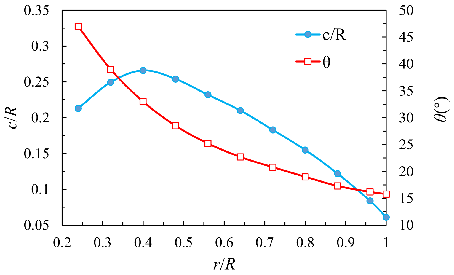
Figure 3.
Chord and pitch distributions of the test propeller.
Figure 3.
Chord and pitch distributions of the test propeller.
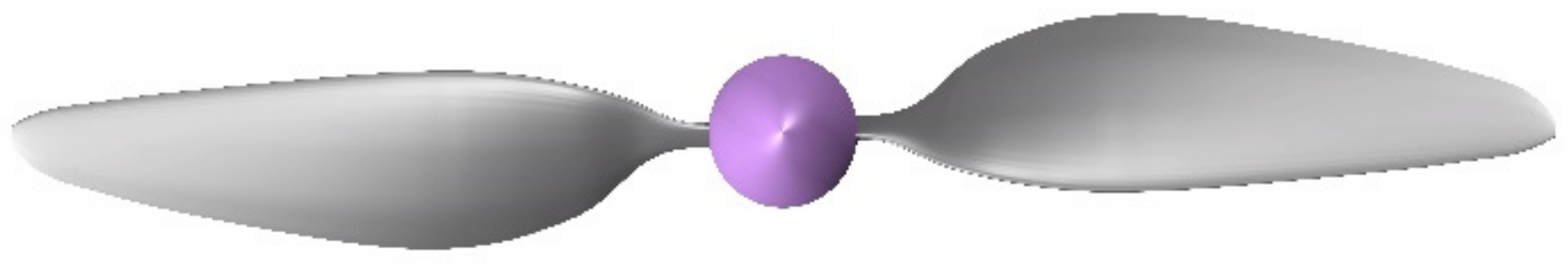
Figure 4.
Three-dimensional shape of the test propeller.
Figure 4.
Three-dimensional shape of the test propeller.
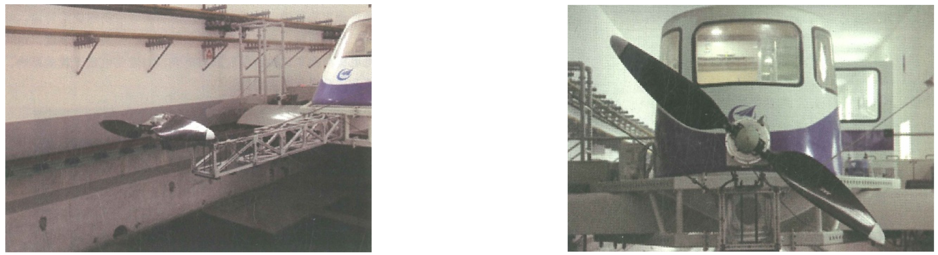
Figure 5.
Ground experiment of the test propeller.
Figure 5.
Ground experiment of the test propeller.
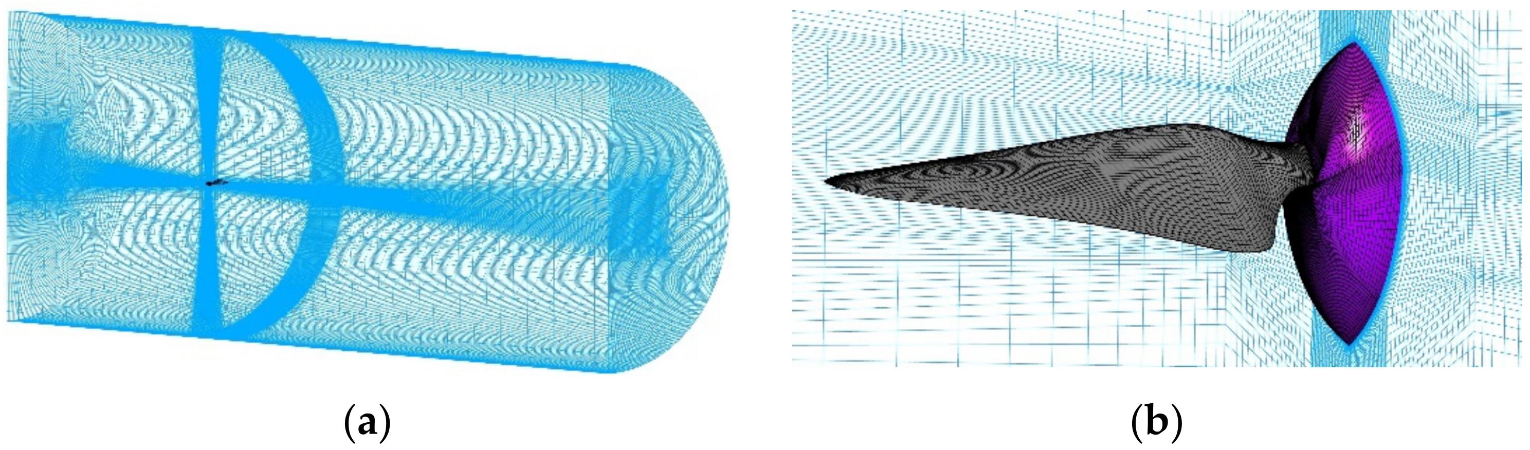
Figure 6.
Computational mesh of the test propeller: (a) Computational domain; (b) Near-wall grids distribution.
Figure 6.
Computational mesh of the test propeller: (a) Computational domain; (b) Near-wall grids distribution.
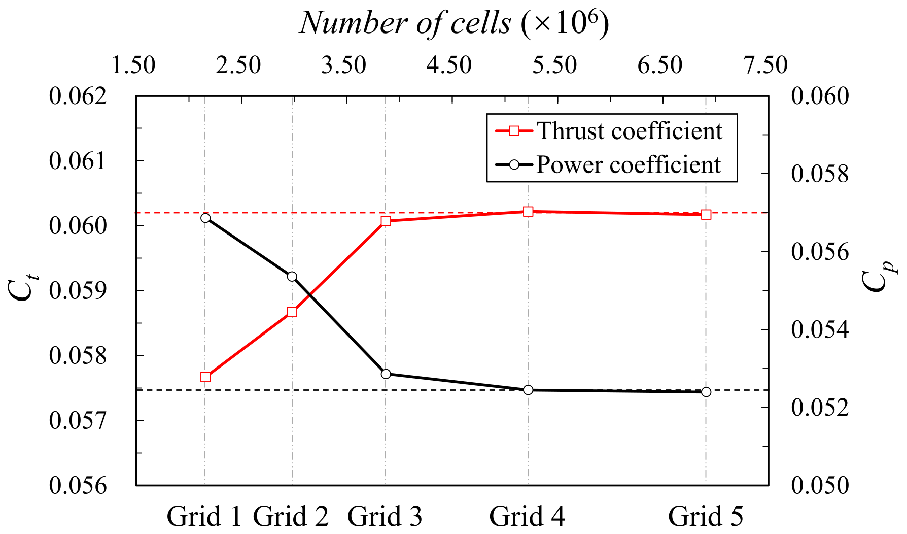
Figure 7.
Comparison of calculation results of five grids.
Figure 7.
Comparison of calculation results of five grids.
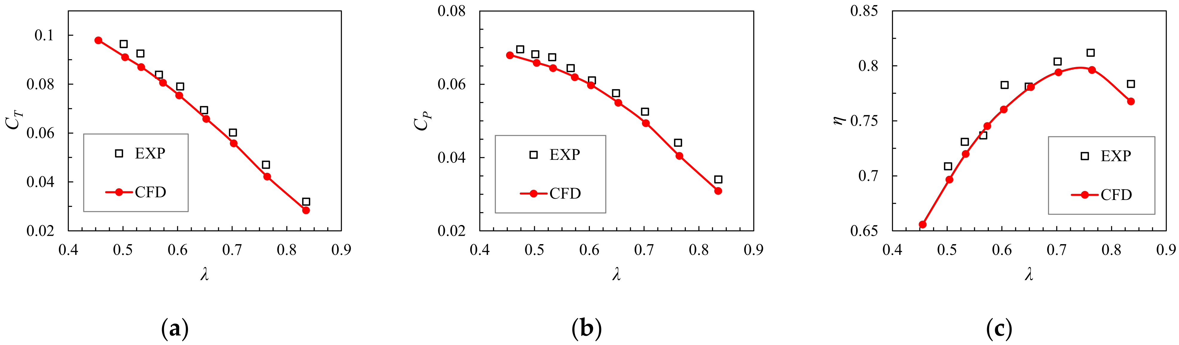
Figure 8.
Experimental data and CFD results at an altitude of 10 km: (a) Thrust coefficient vs. advance ratio; (b) Power coefficient vs. advance ratio; (c) Propeller efficiency vs. advance ratio.
Figure 8.
Experimental data and CFD results at an altitude of 10 km: (a) Thrust coefficient vs. advance ratio; (b) Power coefficient vs. advance ratio; (c) Propeller efficiency vs. advance ratio.
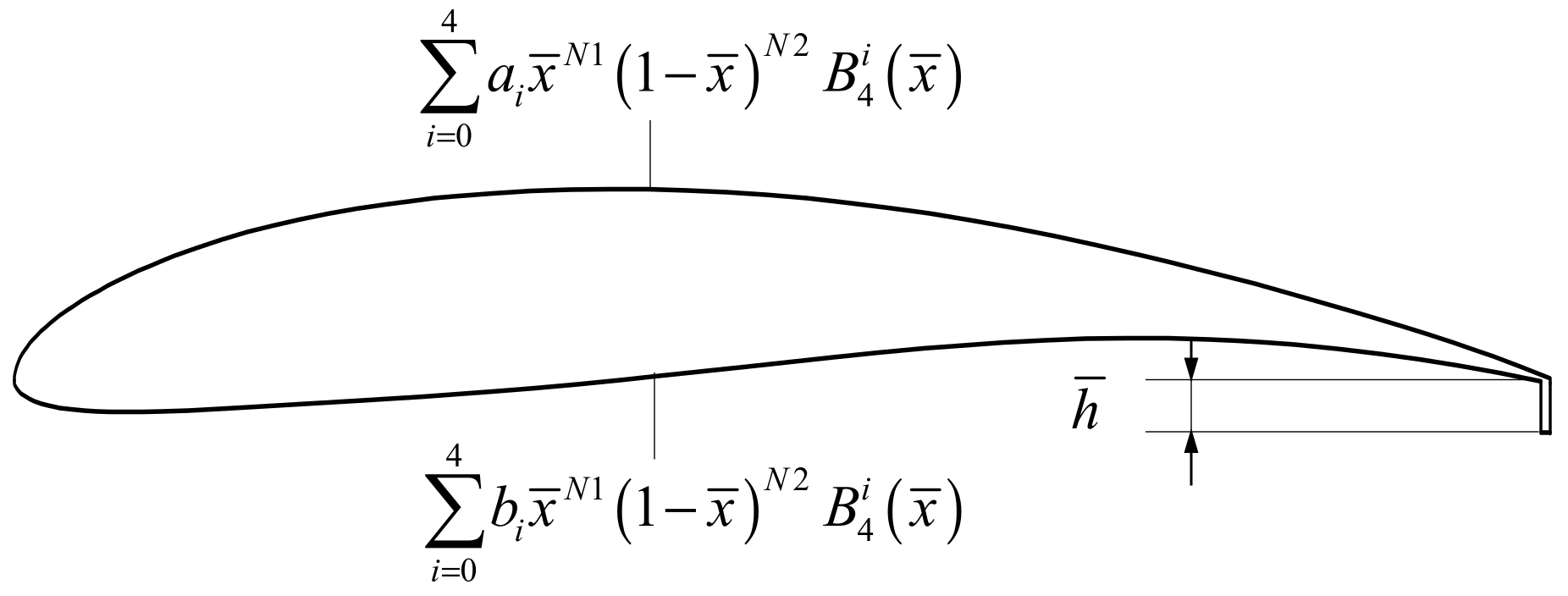
Figure 9.
Parametric method for a Gurney flap airfoil.
Figure 9.
Parametric method for a Gurney flap airfoil.
Figure 10.
Force diagram for a blade element.
Figure 10.
Force diagram for a blade element.
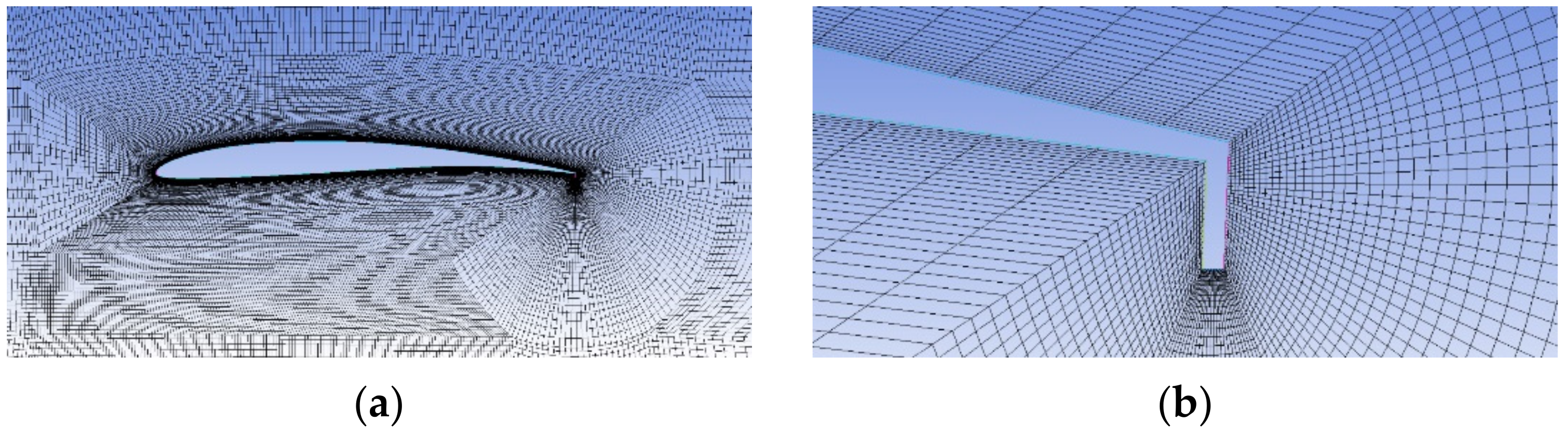
Figure 11.
Computation grid of the cross-sectional airfoil with a Gurney flap: (a) Grid around the airfoil; (b) Grid near the Gurney flap.
Figure 11.
Computation grid of the cross-sectional airfoil with a Gurney flap: (a) Grid around the airfoil; (b) Grid near the Gurney flap.
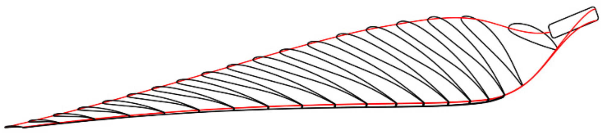
Figure 12.
Parametric method for the propeller with a Gurney flap.
Figure 12.
Parametric method for the propeller with a Gurney flap.
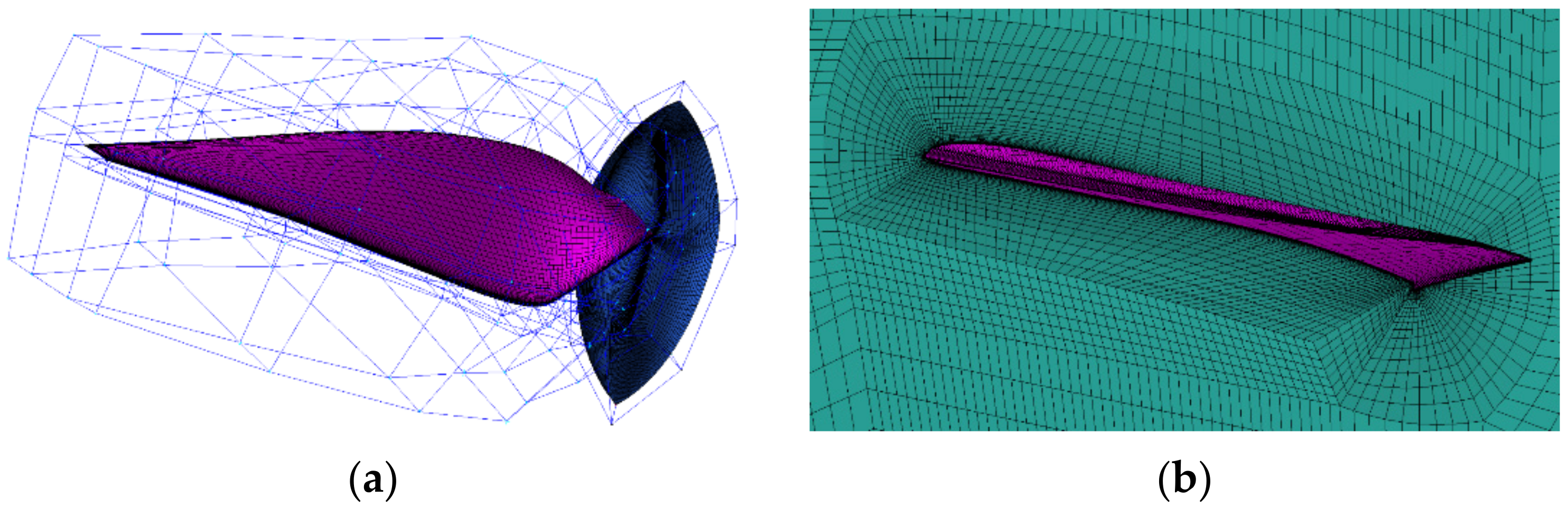
Figure 13.
Computation grid of the propeller with a Gurney flap: (a) Adjustable blocks around the propeller; (b) Grid around cross-sectional airfoil with a Gurney flap.
Figure 13.
Computation grid of the propeller with a Gurney flap: (a) Adjustable blocks around the propeller; (b) Grid around cross-sectional airfoil with a Gurney flap.
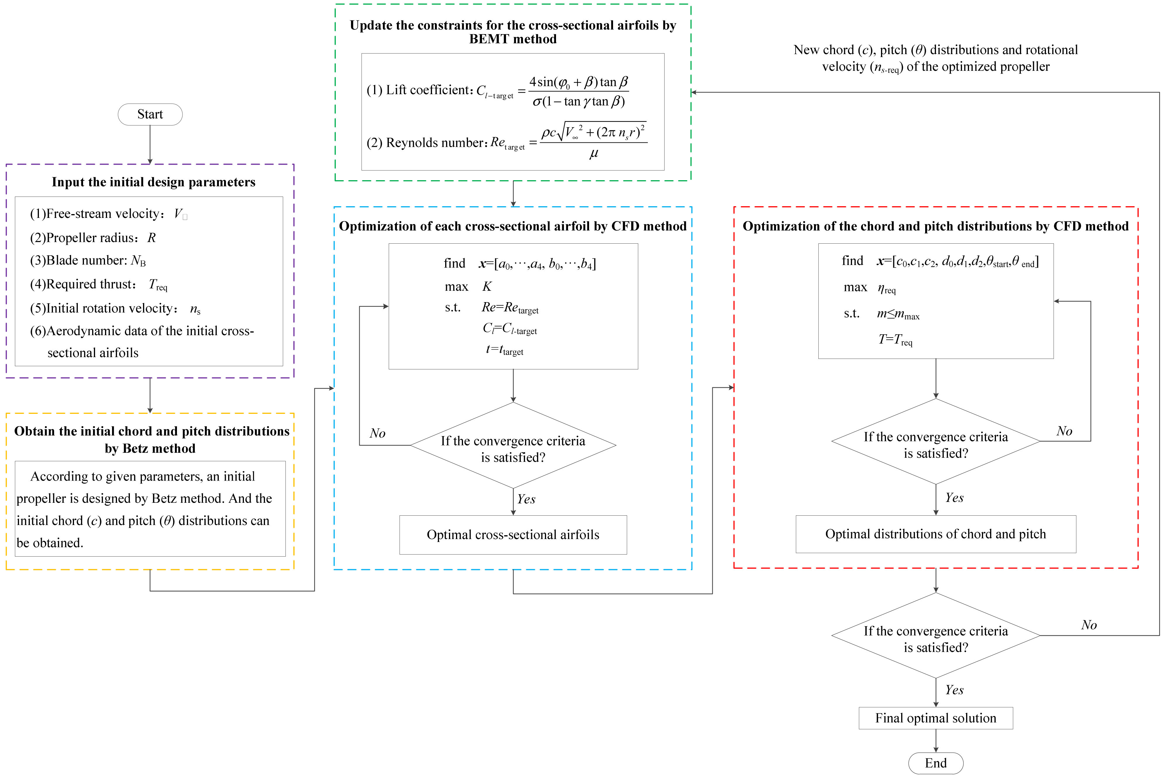
Figure 14.
Flowchart of iterative optimization strategy for low Reynolds number propeller.
Figure 14.
Flowchart of iterative optimization strategy for low Reynolds number propeller.
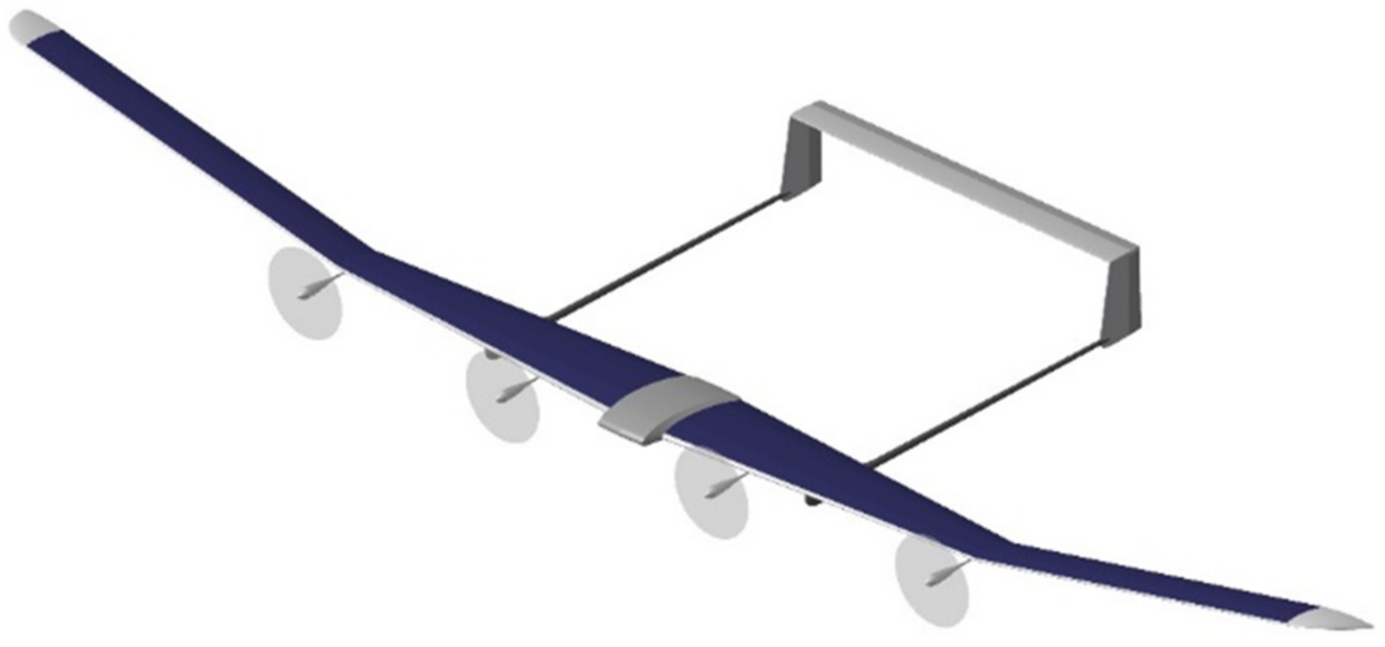
Figure 15.
The ultra-high-altitude unmanned aerial vehicle for case study.
Figure 15.
The ultra-high-altitude unmanned aerial vehicle for case study.
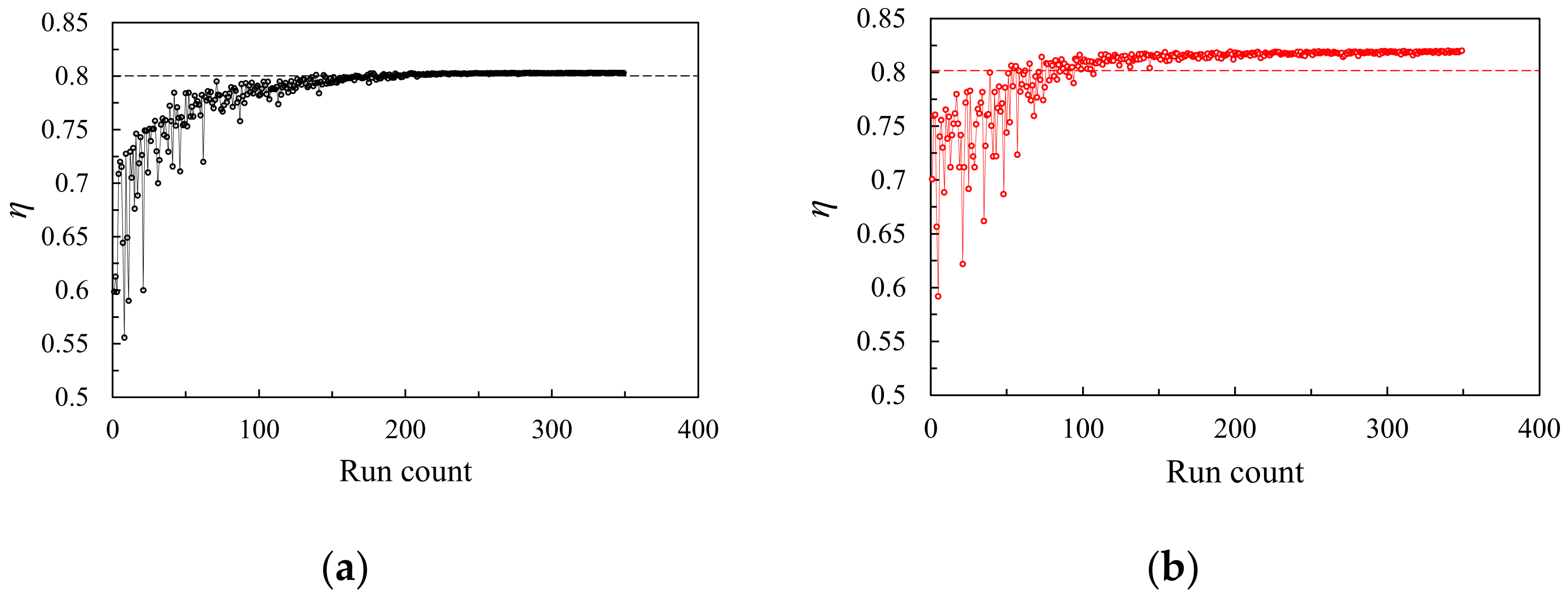
Figure 16.
Convergence history of two optimized propellers in the optimization of chord and pitch distribution: (a) Prop A; (b) Prop B.
Figure 16.
Convergence history of two optimized propellers in the optimization of chord and pitch distribution: (a) Prop A; (b) Prop B.
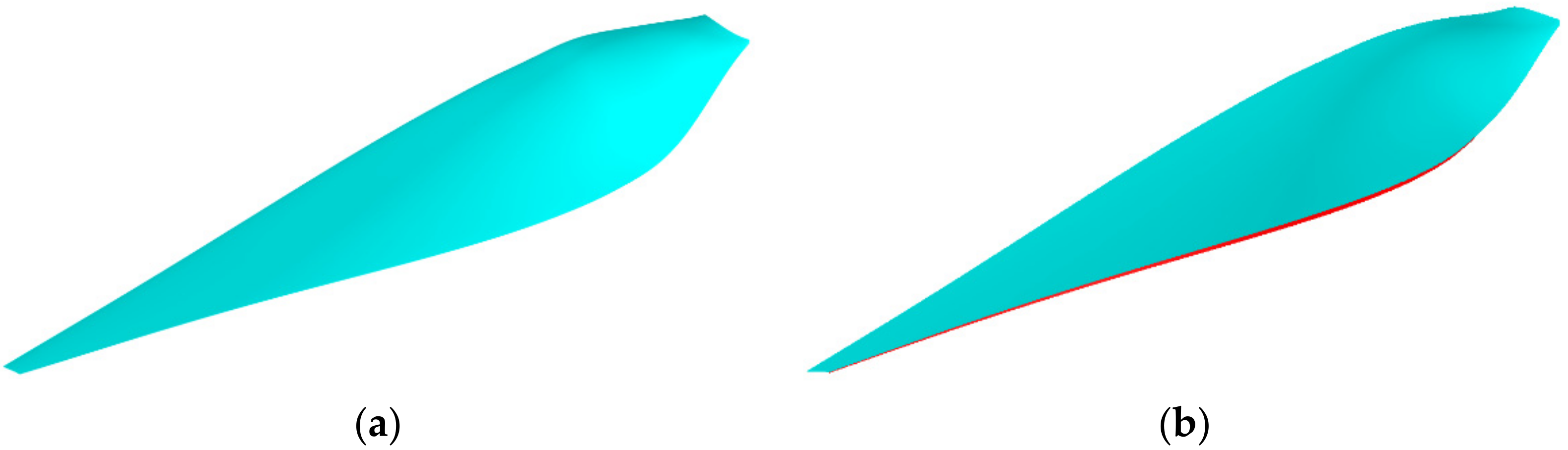
Figure 17.
The geometries of the optimized propellers: (a) Prop A; (b) Prop B.
Figure 17.
The geometries of the optimized propellers: (a) Prop A; (b) Prop B.
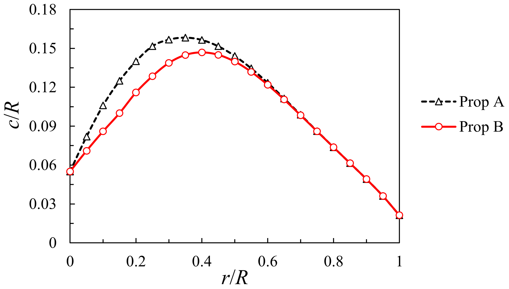
Figure 18.
Blade chord distribution of the two optimized propellers.
Figure 18.
Blade chord distribution of the two optimized propellers.
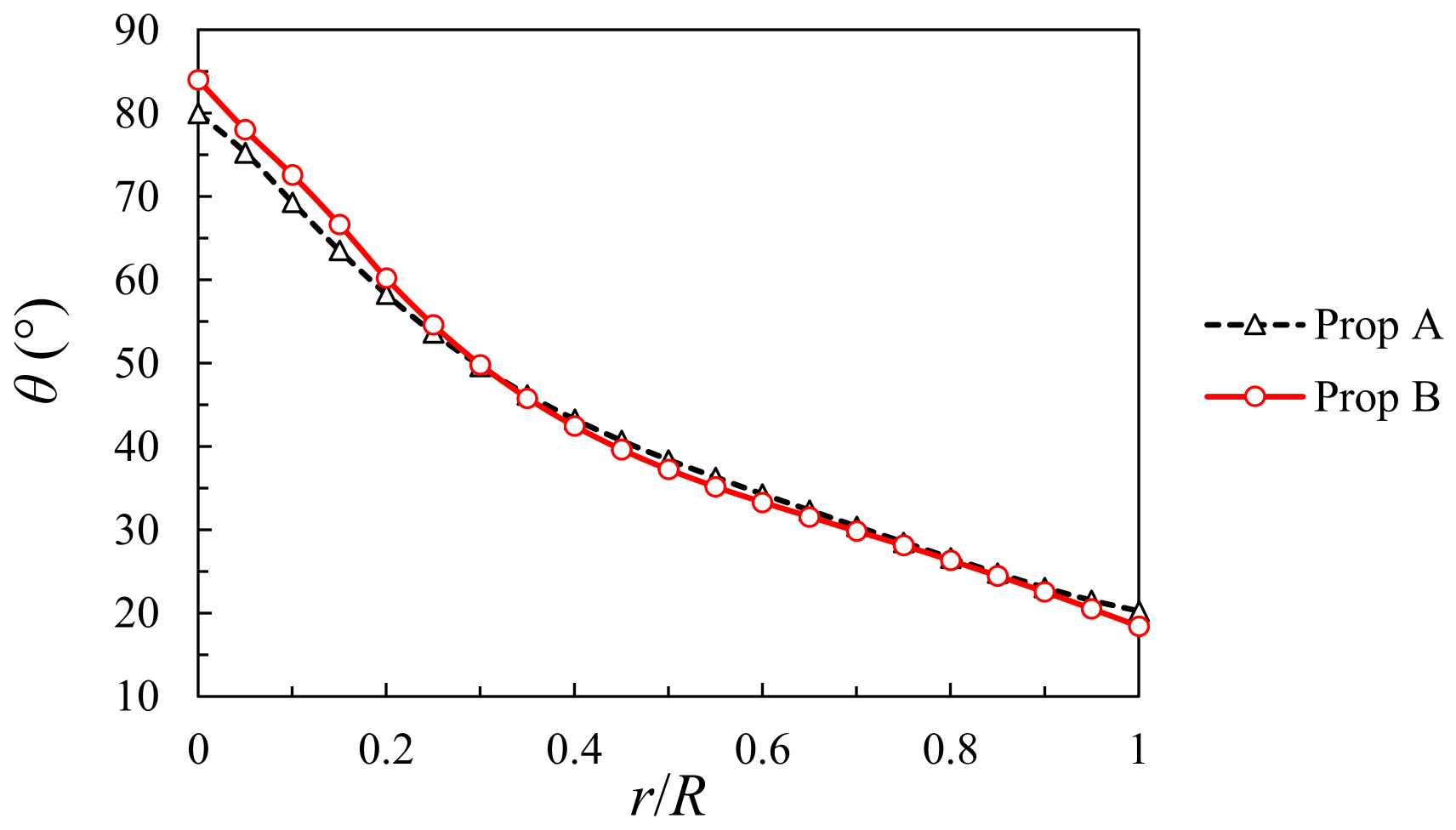
Figure 19.
Blade pitch distribution of the two optimized propellers.
Figure 19.
Blade pitch distribution of the two optimized propellers.
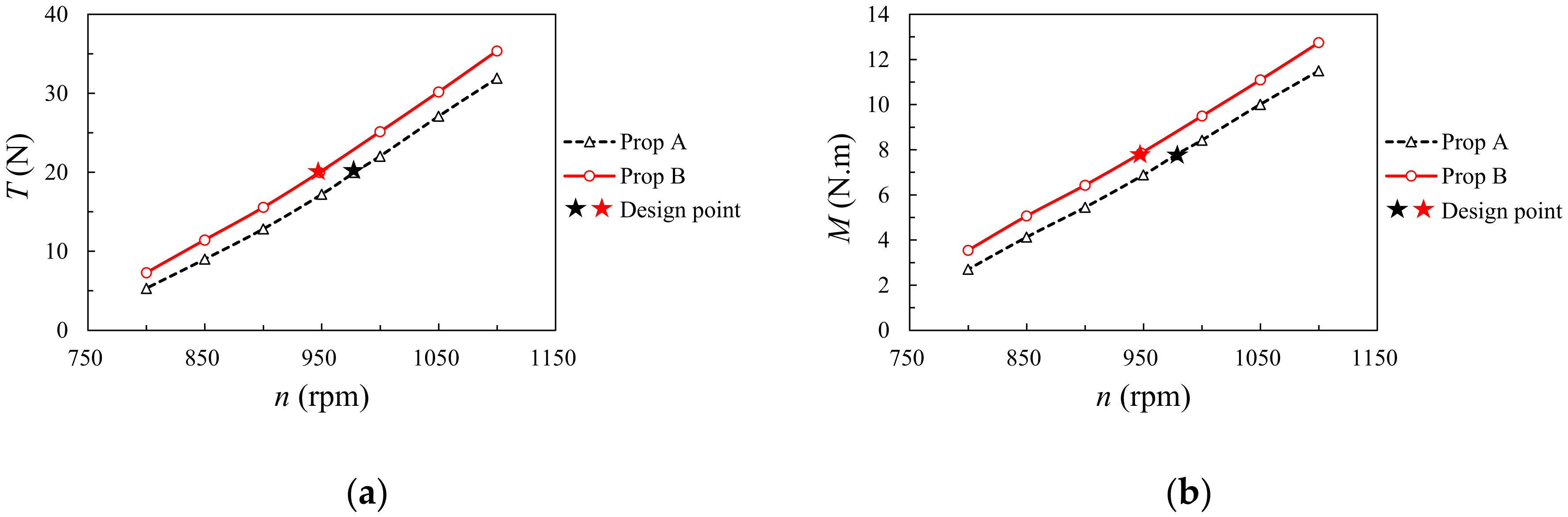
Figure 20.
Aerodynamic performances of Prop A and Prop B near the design point: (a) Thrust vs. rotational velocity; (b) Torque vs. rotational velocity; (c) Efficiency vs. advance ratio; (d) Efficiency vs. thrust.
Figure 20.
Aerodynamic performances of Prop A and Prop B near the design point: (a) Thrust vs. rotational velocity; (b) Torque vs. rotational velocity; (c) Efficiency vs. advance ratio; (d) Efficiency vs. thrust.
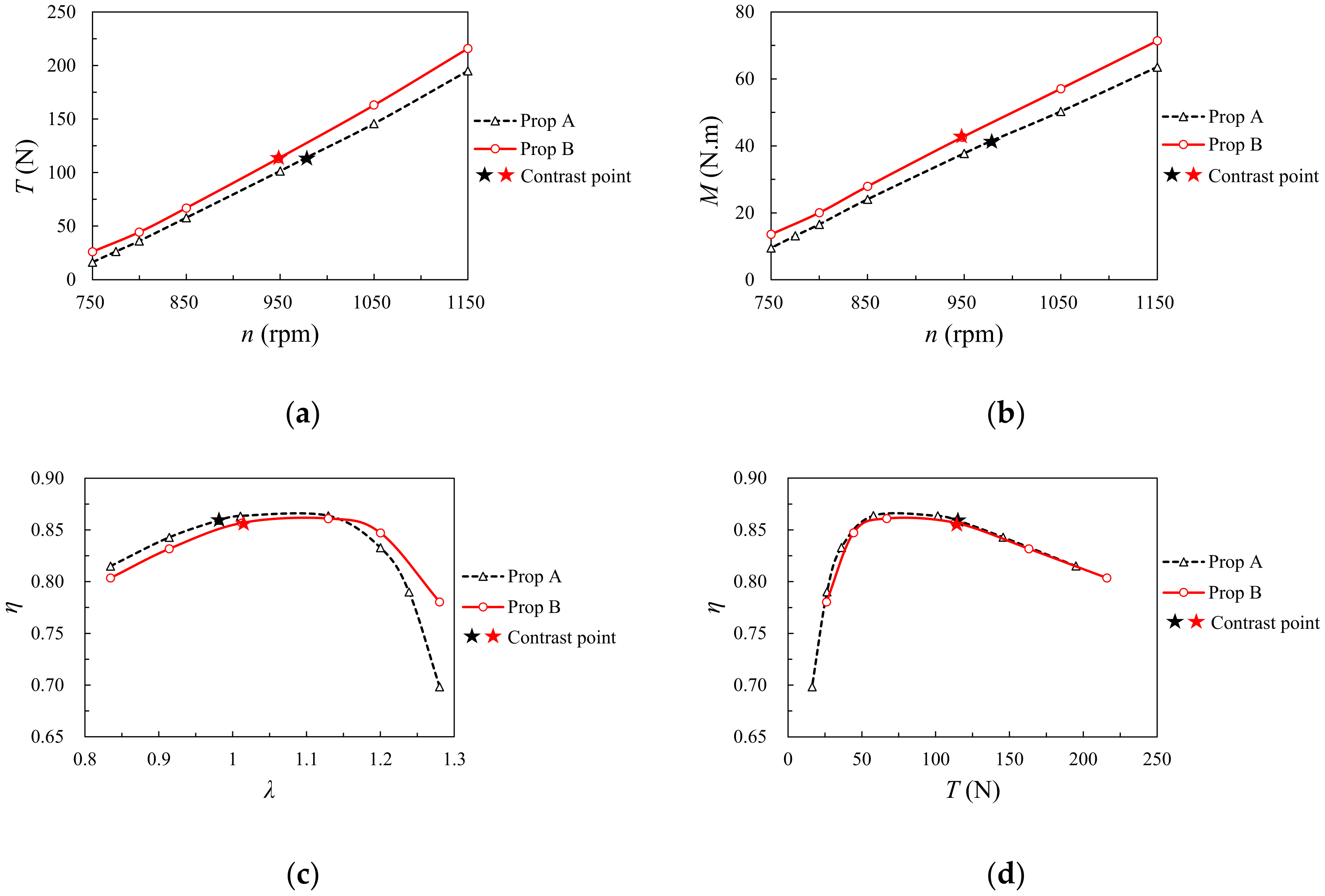
Figure 21.
Aerodynamic performances of two optimized propellers under an average Reynolds number of about 1.8 × 10⁵: (a) Thrust vs. rotational velocity; (b) Torque vs. rotational velocity; (c) Efficiency vs. advance ratio; (d) Efficiency vs. thrust.
Figure 21.
Aerodynamic performances of two optimized propellers under an average Reynolds number of about 1.8 × 10⁵: (a) Thrust vs. rotational velocity; (b) Torque vs. rotational velocity; (c) Efficiency vs. advance ratio; (d) Efficiency vs. thrust.
Figure 22.
Aerodynamic performances of Prop A and Prop B at their design advance ratios.
Figure 22.
Aerodynamic performances of Prop A and Prop B at their design advance ratios.
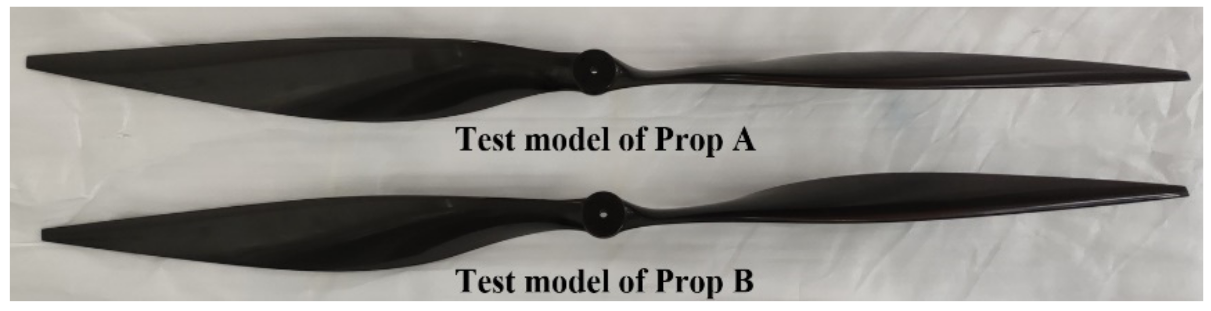
Figure 24.
The test models.
Figure 24.
The test models.
Figure 25.
The detail of the Gurney flap on the test model.
Figure 25.
The detail of the Gurney flap on the test model.
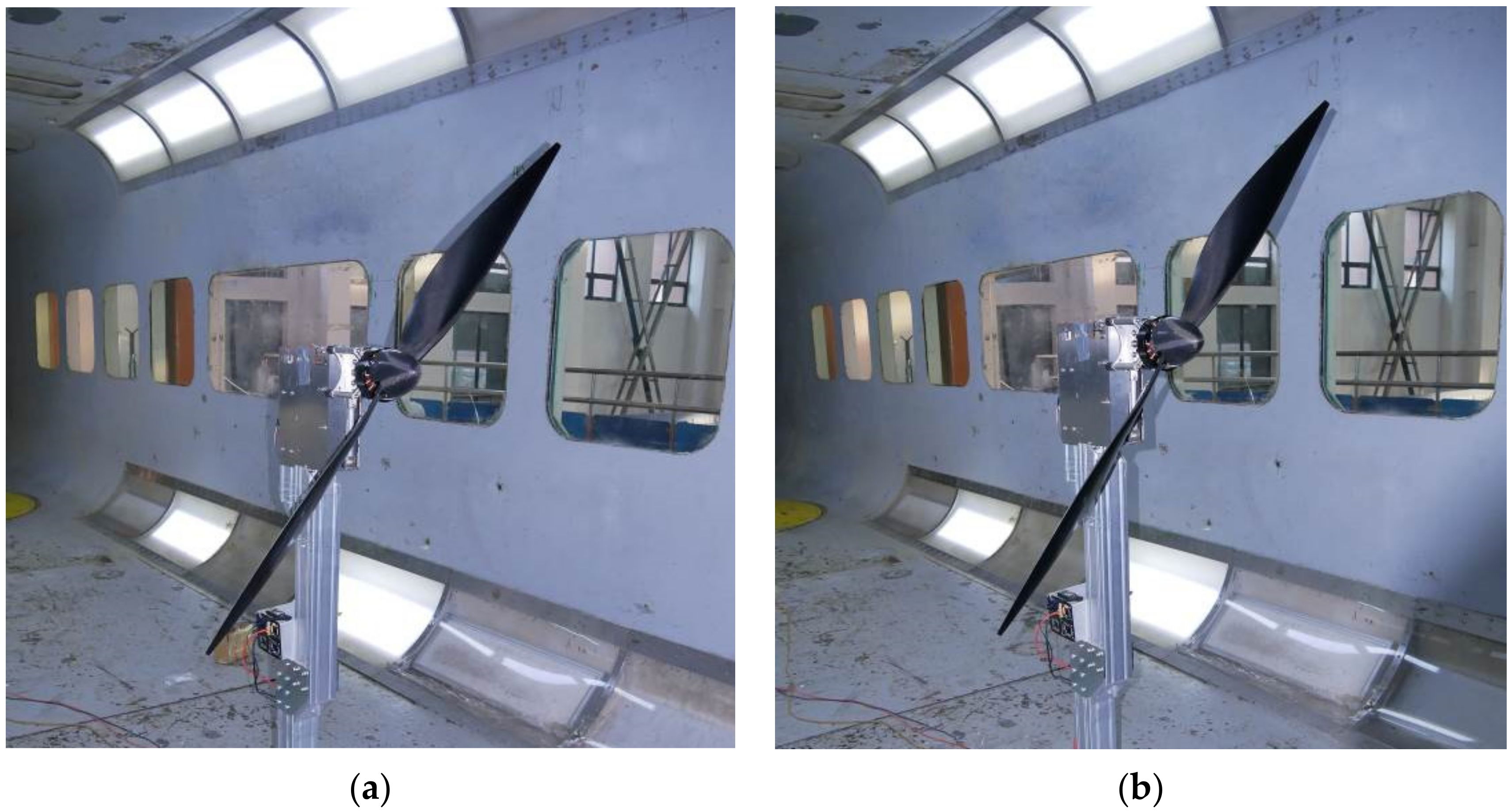
Figure 26.
Test propellers installed in the wind tunnel: (a) The test propeller without a Gurney flap (Prop A); (b) The test propeller with a Gurney flap (Prop B).
Figure 26.
Test propellers installed in the wind tunnel: (a) The test propeller without a Gurney flap (Prop A); (b) The test propeller with a Gurney flap (Prop B).
Figure 27.
Results of the repeated test: (a) Thrust coefficient vs. advance ratio; (b) Power coefficient vs. advance ratio.
Figure 27.
Results of the repeated test: (a) Thrust coefficient vs. advance ratio; (b) Power coefficient vs. advance ratio.
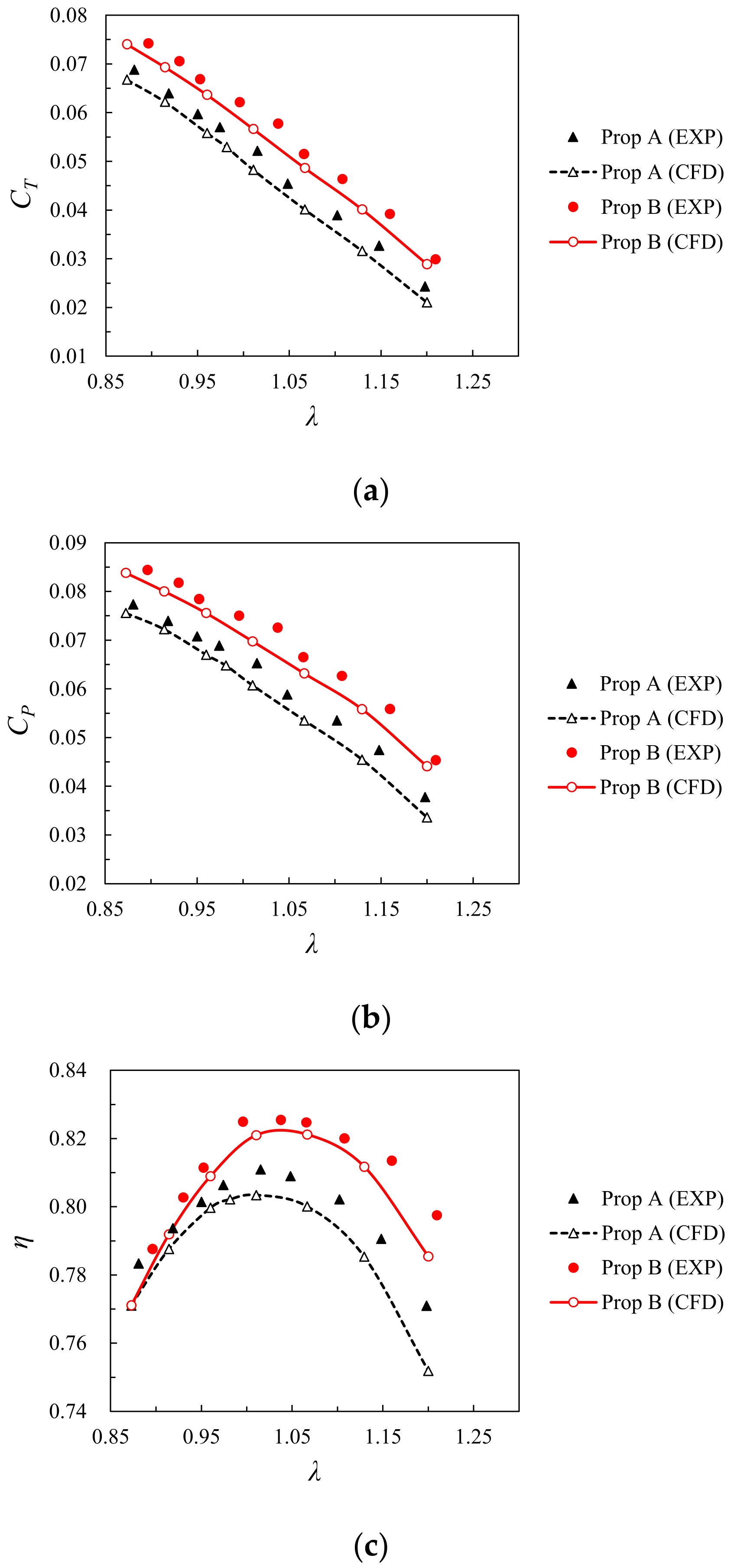
Figure 28.
Comparison of the test and CFD results under Re ≈ 4 × 10⁴: (a) Thrust coefficient vs. advance ratio; (b) Power coefficient vs. advance ratio; (c) Propeller efficiency vs. advance ratio.
Figure 28.
Comparison of the test and CFD results under Re ≈ 4 × 10⁴: (a) Thrust coefficient vs. advance ratio; (b) Power coefficient vs. advance ratio; (c) Propeller efficiency vs. advance ratio.
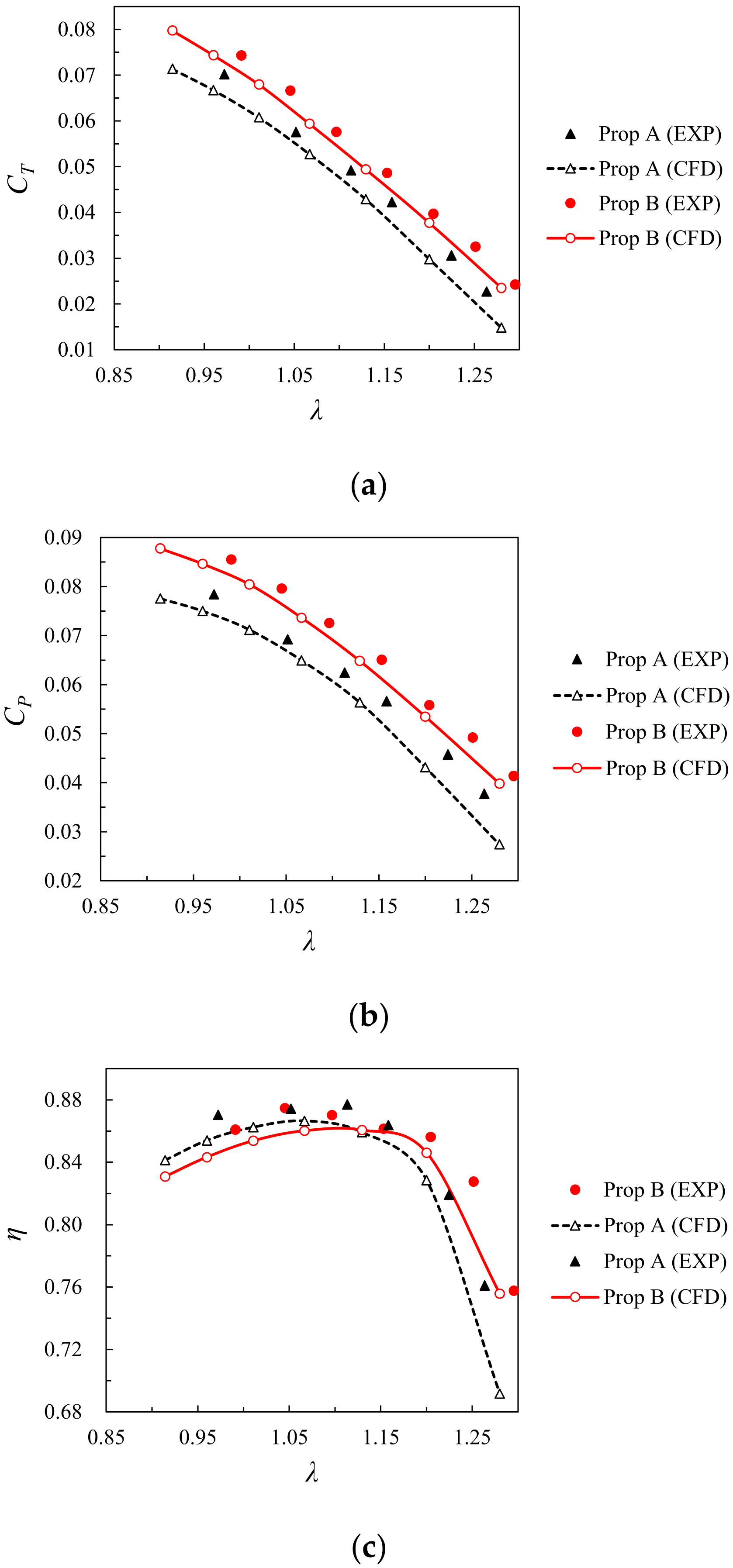
Figure 29.
Comparison of the test and CFD results under Re ≈ 1.6 × 10⁵: (a) Thrust coefficient vs. advance ratio; (b) Power coefficient vs. advance ratio; (c) Propeller efficiency vs. advance ratio.
Figure 29.
Comparison of the test and CFD results under Re ≈ 1.6 × 10⁵: (a) Thrust coefficient vs. advance ratio; (b) Power coefficient vs. advance ratio; (c) Propeller efficiency vs. advance ratio.
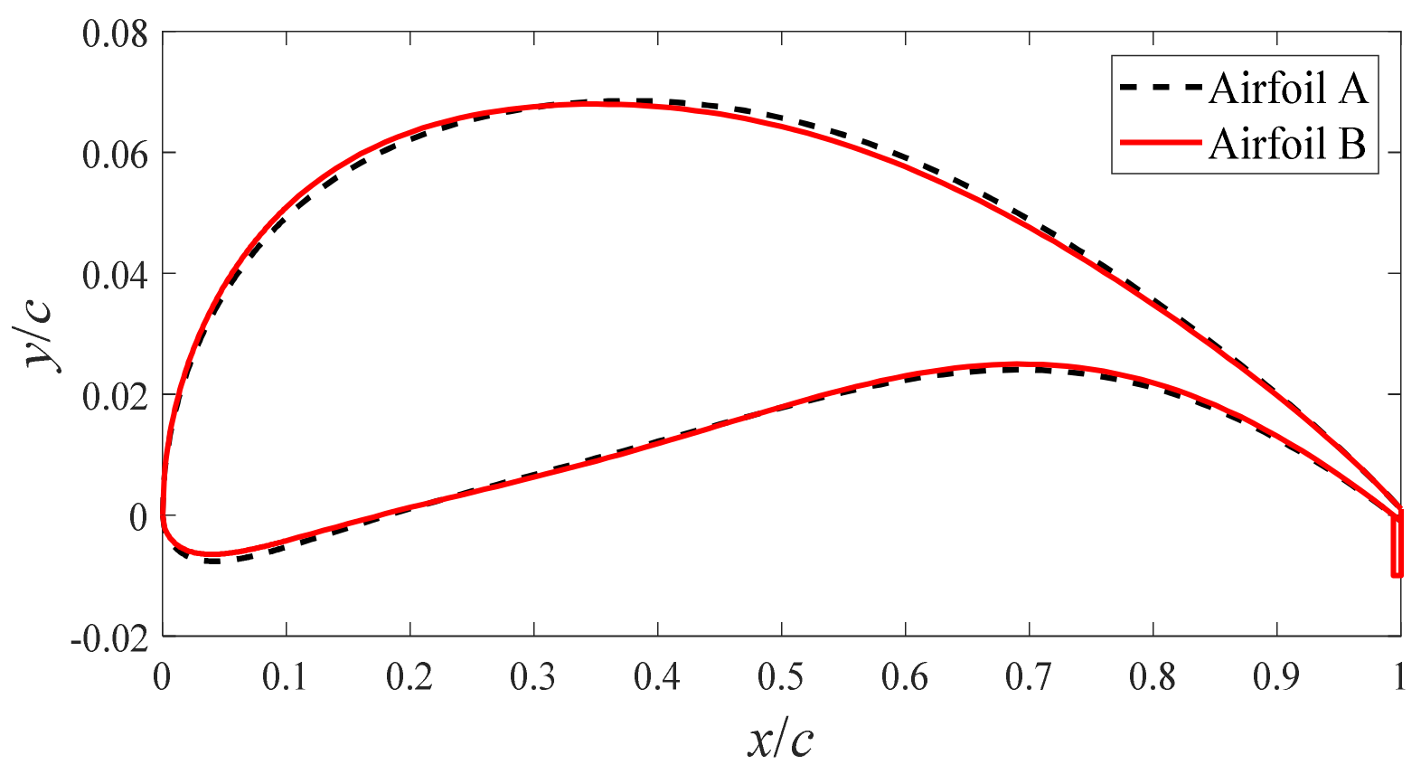
Figure 30.
Geometries of the cross-sectional airfoils on Prop A and Prop B at 0.75 R.
Figure 30.
Geometries of the cross-sectional airfoils on Prop A and Prop B at 0.75 R.
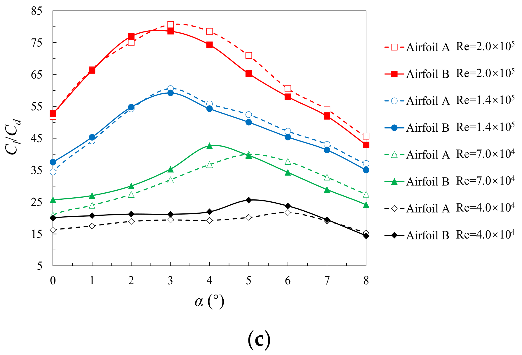
Figure 31.
Aerodynamic performance of Airfoil A, and Airfoil B at different Reynolds numbers: (a) Lift coefficient vs. angle of attack; (b) Drag coefficient vs. angle of attack; (c) Lift-to-drag ratio vs. angle of attack.
Figure 31.
Aerodynamic performance of Airfoil A, and Airfoil B at different Reynolds numbers: (a) Lift coefficient vs. angle of attack; (b) Drag coefficient vs. angle of attack; (c) Lift-to-drag ratio vs. angle of attack.
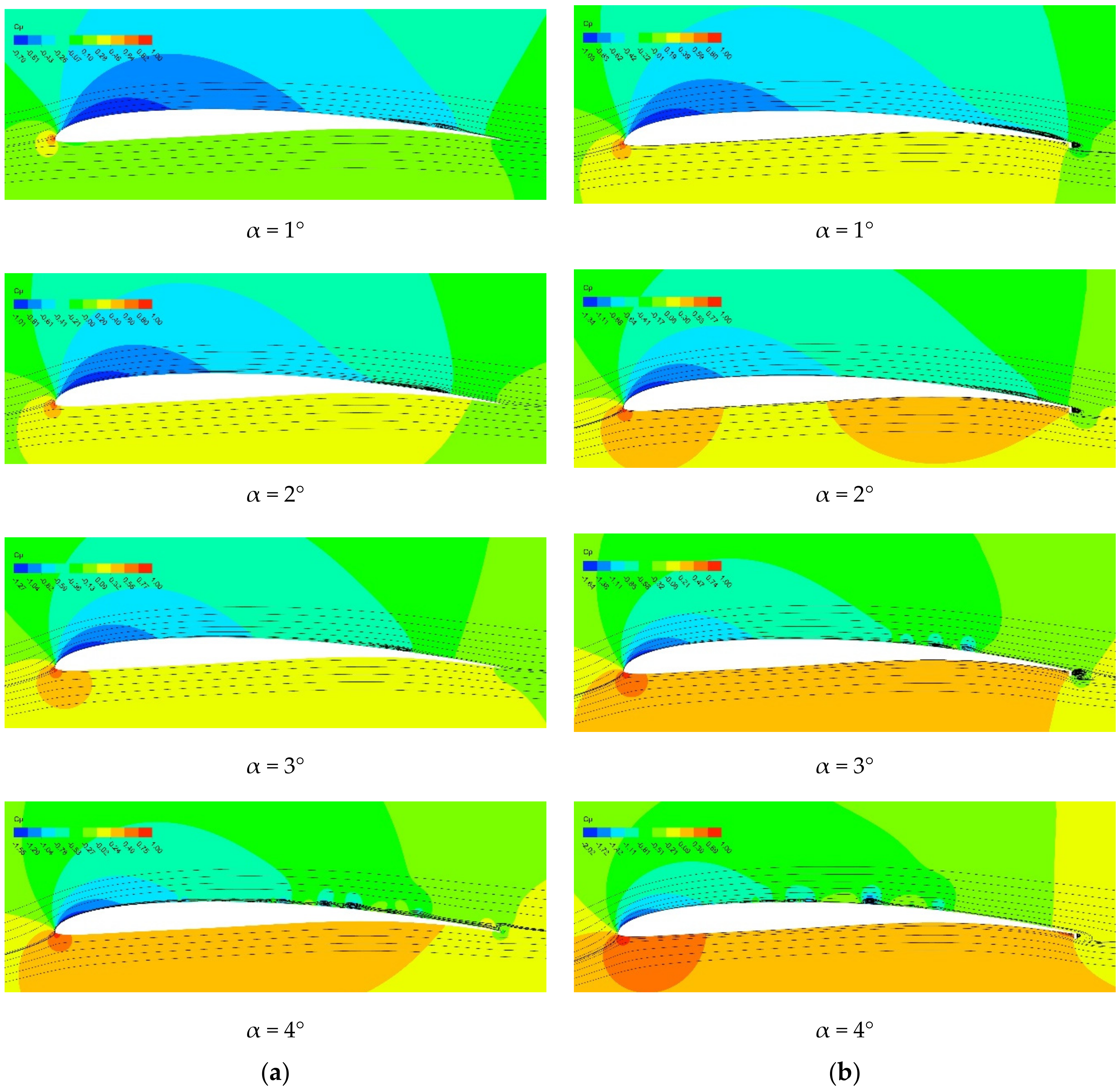
Figure 32.
Pressure coefficient and streamline distributions at Re = 4.0 × 10⁴: (a) Airfoil A; (b) Airfoil B.
Figure 32.
Pressure coefficient and streamline distributions at Re = 4.0 × 10⁴: (a) Airfoil A; (b) Airfoil B.
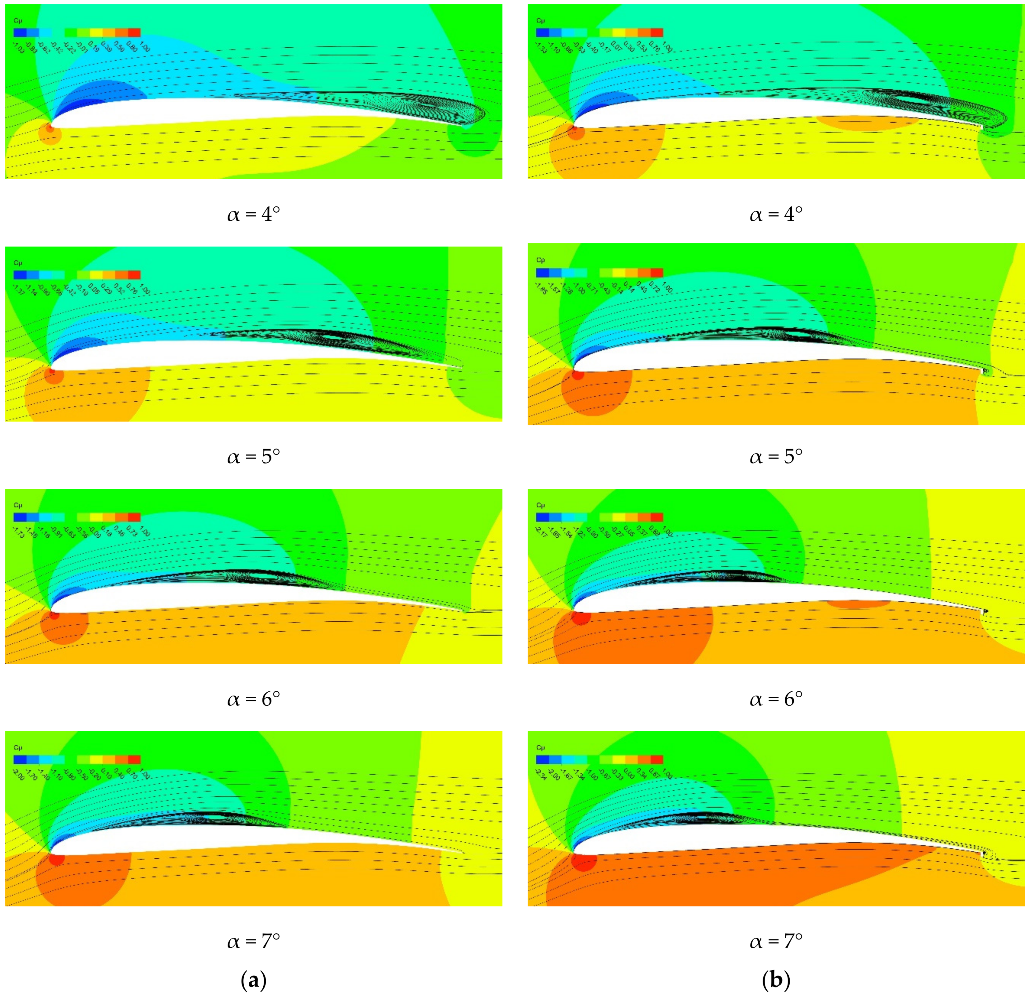
Figure 33.
Pressure coefficient and streamline distributions at Re = 2.0 × 10⁵: (a) Airfoil A; (b) Airfoil B.
Figure 33.
Pressure coefficient and streamline distributions at Re = 2.0 × 10⁵: (a) Airfoil A; (b) Airfoil B.
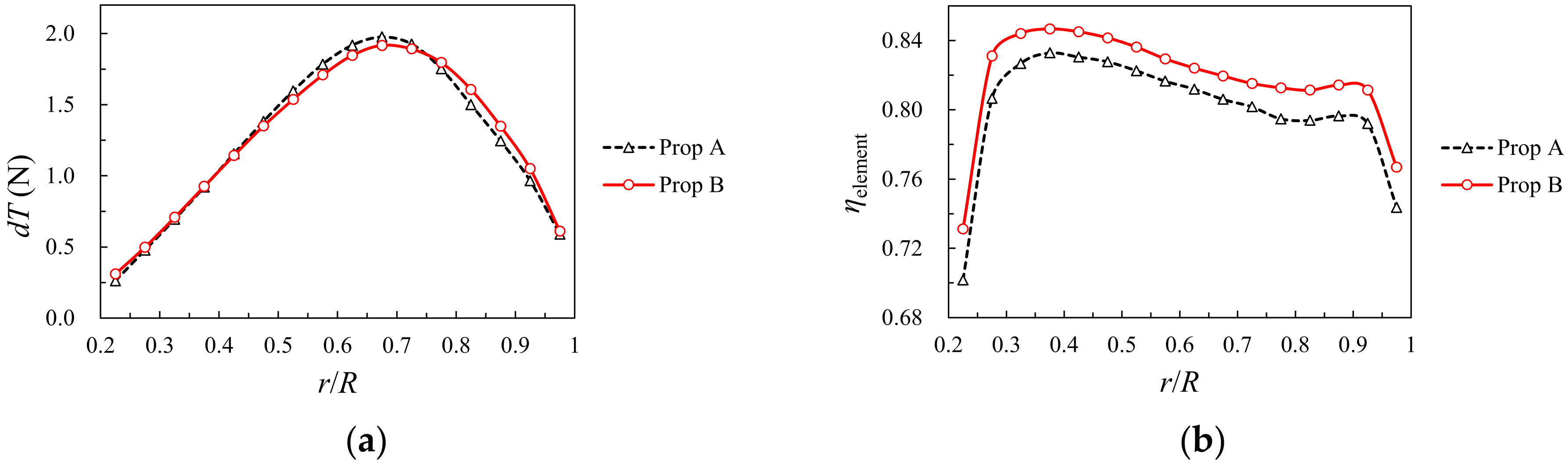
Figure 34.
Aerodynamic characteristics along the blade of two propellers at State 1: (a) Distributions of blade element thrust; (b) Distributions of blade element efficiency.
Figure 34.
Aerodynamic characteristics along the blade of two propellers at State 1: (a) Distributions of blade element thrust; (b) Distributions of blade element efficiency.
Figure 35.
Aerodynamic characteristics along the blade of two propellers at State 2: (a) Distributions of blade element thrust; (b) Distributions of blade element efficiency.
Figure 35.
Aerodynamic characteristics along the blade of two propellers at State 2: (a) Distributions of blade element thrust; (b) Distributions of blade element efficiency.
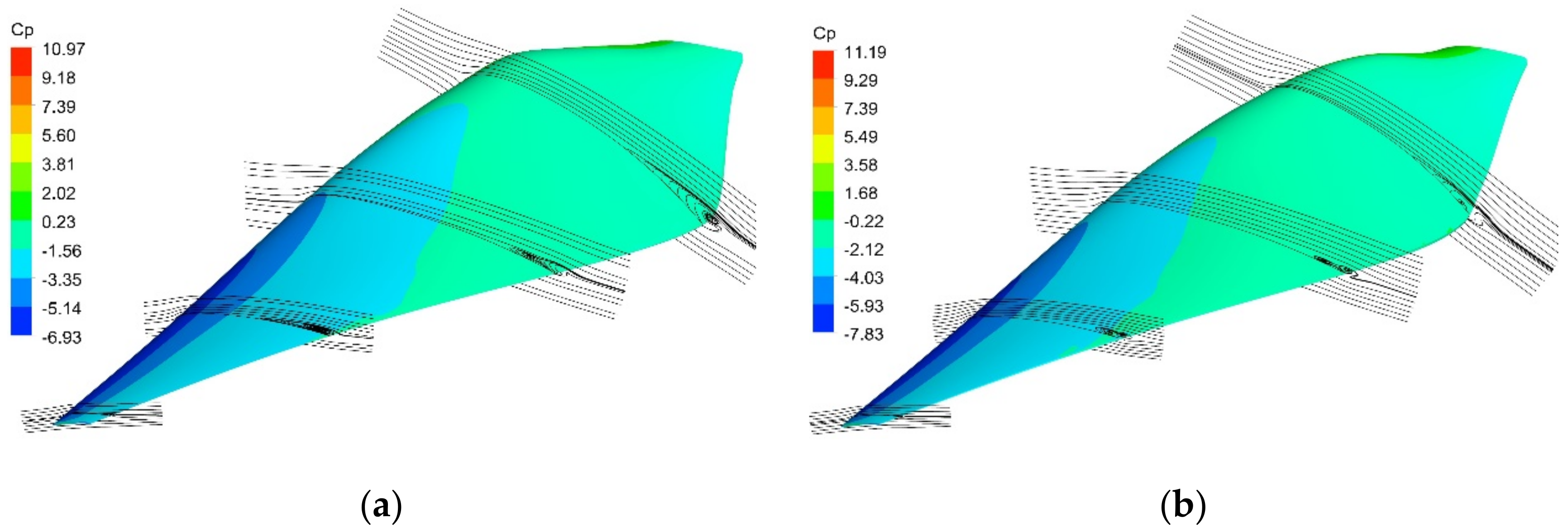
Figure 36.
Pressure coefficient distribution and streamlines on different cross-sections of two propellers at State 1: (a) Prop A; (b) Prop B.
Figure 36.
Pressure coefficient distribution and streamlines on different cross-sections of two propellers at State 1: (a) Prop A; (b) Prop B.
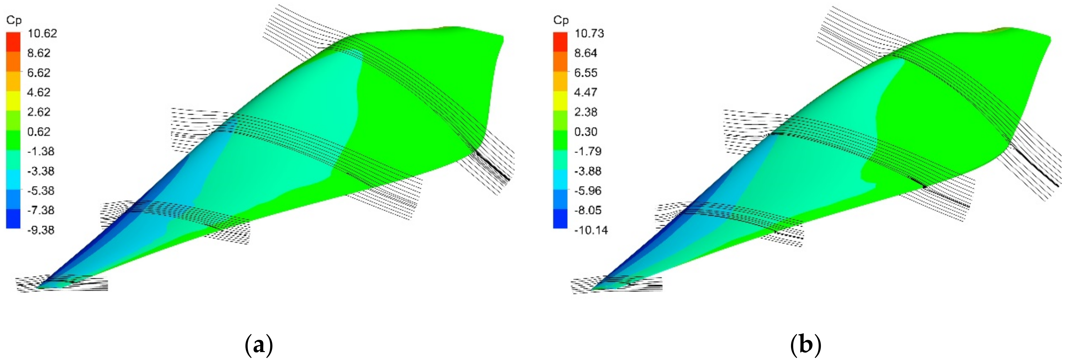
Figure 37.
Pressure coefficient distribution and streamlines on different cross-sections of two propellers at State 2: (a) Prop A; (b) Prop B.
Figure 37.
Pressure coefficient distribution and streamlines on different cross-sections of two propellers at State 2: (a) Prop A; (b) Prop B.
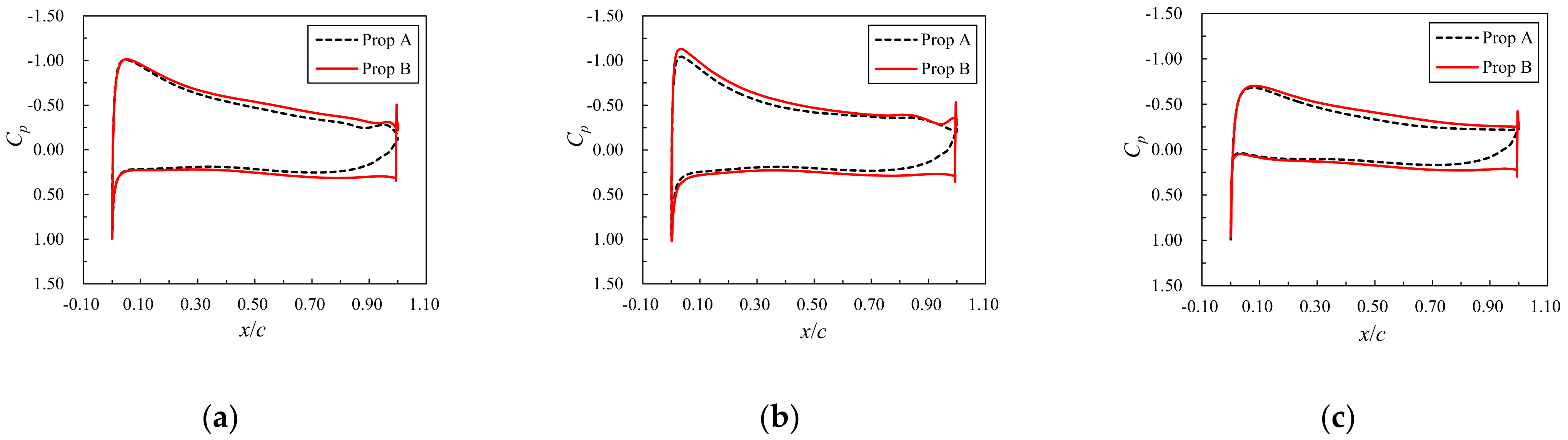
Figure 38.
Pressure coefficient distribution on different cross-sectional airfoils at State 1: (a) r/R = 0.5; (b) r/R = 0.75; (c) r/R = 0.95.
Figure 38.
Pressure coefficient distribution on different cross-sectional airfoils at State 1: (a) r/R = 0.5; (b) r/R = 0.75; (c) r/R = 0.95.
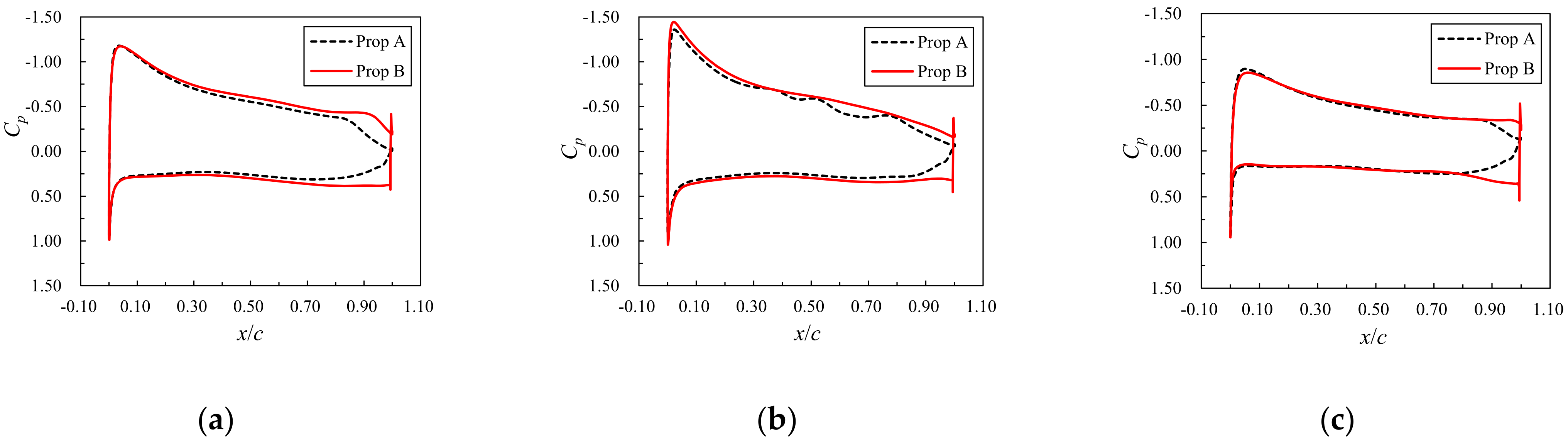
Figure 39.
Pressure coefficient distribution on different cross-sectional airfoils at State 2: (a) r/R = 0.5; (b) r/R = 0.75; (c) r/R = 0.95.
Figure 39.
Pressure coefficient distribution on different cross-sectional airfoils at State 2: (a) r/R = 0.5; (b) r/R = 0.75; (c) r/R = 0.95.
Table 1.
Test conditions and parameters of the test model.
Table 1.
Test conditions and parameters of the test model.
| Span (m) | c (m) | Ma | P (kPa) | Re |
|---|
| 0.9144 | 0.1524 | 0.05 | 34.475 | 1.0 × 10⁵ |
Table 2.
Relation between the test states and flight states of the test propeller.
Table 2.
Relation between the test states and flight states of the test propeller.
| Altitude (km) | λ | Reaverage | Flight States | Test States |
|---|
| Vꝏ (m/s) | n (rpm) | Vꝏ (m/s) | n (rpm) |
|---|
| 10 | 0.78 | 1.55 × 10⁵ | 14.1 | 542 | 5.84 | 225 |
| 0.68 | 1.73 × 10⁵ | 622 | 258 |
| 0.58 | 1.98 × 10⁵ | 729 | 302 |
Table 3.
Test conditions and parameters of the test model.
Table 3.
Test conditions and parameters of the test model.
| Grid | Number of Spanwise Nodes | Number of Chordal Nodes | Number of Cells |
|---|
| Grid 1 | 60 | 15 | 2.16 × 10⁶ |
| Grid 2 | 80 | 30 | 2.98 × 10⁶ |
| Grid 3 | 100 | 45 | 3.87 × 10⁶ |
| Grid 4 | 120 | 60 | 5.22 × 10⁶ |
| Grid 5 | 140 | 75 | 6.91 × 10⁶ |
Table 4.
Parameters of propeller and the design state.
Table 4.
Parameters of propeller and the design state.
| NB | D (m) | Vꝏ (m/s) | Ρ (kg/m3) | μ (Ns/m2) | Treq (N) |
|---|
| 2 | 2 | 32 | 0.0889 | 1.422 × 10⁻⁵ | 20 |
Table 5.
Comparison between two optimized propellers at the design point.
Table 5.
Comparison between two optimized propellers at the design point.
| Propeller | Treq(N) | n (rpm) | λ | η | Reaverage |
|---|
| Prop A | 20 | 978 | 0.9816 | 80.2% | 4.2 × 10⁴ |
| Prop B | 20 | 948 | 1.0105 | 82.0% | 4.0 × 10⁴ |
Table 6.
Comparison between two optimized propellers at the design point.
Table 6.
Comparison between two optimized propellers at the design point.
| Vꝏ (m/s) | n (rpm) | λ | Reaverage |
|---|
| Prop A | Prop B |
|---|
| 4.2 | 150 | 1.20 | 3.7 × 10⁴ | 3.5 × 10⁴ |
| 178 | 1.01 | 4.2 × 10⁴ | 4.0 × 10⁴ |
| 206 | 0.87 | 4.6 × 10⁴ | 4.4 × 10⁴ |
| 16.0 | 577 | 1.20 | 1.4 × 10⁵ | 1.4 × 10⁵ |
| 685 | 1.01 | 1.6 × 10⁵ | 1.5 × 10⁵ |
| 700 | 0.98 | 1.8 × 10⁵ | 1.7 × 10⁵ |
Table 7.
Performances of two optimized propellers at the states with different Reynolds numbers.
Table 7.
Performances of two optimized propellers at the states with different Reynolds numbers.
| Propeller | Vꝏ (m/s) | State 1 | State 2 |
|---|
| Reaverage | n (rpm) | T (N) | η | Reaverage | n (rpm) | T (N) | η |
|---|
| Prop A | 32 | 4.2 × 10⁴ | 978 | 20 | 80.2% | 1.9 × 10⁵ | 978 | 115 | 86.3% |
| Prop B | 32 | 4.0 × 10⁴ | 948 | 20 | 82.0% | 1.8 × 10⁵ | 948 | 117 | 85.9% |


