Multicriteria Route Planning for In-Operation Mass Transit under Urban Data

Abstract

Multicriteria route planning is a crucial transportation planning issue under the field of GIS-based multicriteria decision analysis (GIS-MCDA) with broad applications. A searching algorithm is proposed to solve the multicriteria route planning problem with spatial urban information and constraints such an existing transit network in operation, certain vertices to be visited in the path, total number of vertices been visited, and length or range for the path. Evaluation of two in-operation mass-transit systems from Chicago and Tainan show that our method can retrieve solutions in a Pareto-optimal sense over comparative methods between profit under queried constraints (the expected passenger flow to be maximized, referring to the social welfare for the public) and cost for construction as well as maintenance (the cost of route to be minimized, referring to the sustainability for the government) with reasonable runtime over comparative methods.

1. Introduction

Constrained planning is ubiquitous in urban design [1]. Many automatic planning or artificial intelligence tasks involving assigning values to variables that are subject to a set of constraints could be formulated as a constraint-satisfaction problem (CSP) [2]. Among CSPs, multicriteria constrained route planning turns out to be one of the most significant research topics with broad applications, especially in the field of transportation [3,4,5,6,7,8], in which the algorithms often have specific or defined heuristic functions.

This research focuses on nonmonotonic multicriteria route planning in urban space, by deploying additional transportation routes for in-operation public transit systems. Employing new services for an in-operation mobility system such as bus or light rail is difficult and time-consuming for governments or public transportation authorities. To be more explicit, factors including, but not limited to, the potential passenger flow (PF), social welfare, road network structure, and fuel consumption need to be considered for this newly deployed service. Furthermore, how to address the transfer as well as competitive relationship between this new service and other existing routes is complex and difficult to quantify. Indeed, even though there are various well-developed traffic planning software (e.g., VISUM, EMME), it is still difficult for authorities to either provide quantitative analysis or present near-optimal plans in a timely manner due to specific requests.

Designing an intelligent route planning algorithm that effectively combines multicriteria factors is also quite challenging. During the route construction process, when an algorithm selects the areas for forming a new route, it will encounter a severe problem: the potential PF of a new route is not monotonic. That is, by viewing the process and the structure of this newly growing route as a spanning tree, instead of increasing the potential profit, adding a new area for this route to cruise might decrease its overall PF as a result of the relationship with in-operation routes and the complex urban functionalities. For instance, a new route with adequate intersections towards the in-operation service can bring passengers to transfer across routes. This not only results in a higher PF, but also enhances the social welfare. On the contrary, when a new route has indistinct boundary against other in-operation services’ areas, its PF could conversely decrease. That is, those who need this service in certain areas with less accessibility cannot benefit from this new deployment, and passengers simply take the original route instead of this new service; both of which thereafter makes this deployment a waste of resources. In this work, considering the complex correlations between locations and stations (e.g., transferring between routes) and heterogeneous urban functions (e.g., the security/scenery of surroundings), an effective route-planning method is proposed to deal with the nonmonotonic multicriteria scenario.

Towards the targeted nonmonotonic multicriteria constrained route planning problem, this paper first harvests heterogeneous input features from Open Street Map (OSM) as well as open data platforms from governments, and then adopts a PF inference [9] for the proposed Multisource Bidirectional Gaussian-Prioritized Spanning Tree (BiasSpan). Precisely, the input constraints from authorities/users include a range on the map, a set of must-visit stations to deploy, maximum length of route, and a number of additional stations to be deployed, and BiasSpan accordingly suggests a route with maximized PF along with a near-optimally minimized cost. The system flow is illustrated in Figure 1.

Evaluation results on two in-operation mass-transit systems from Chicago and Tainan demonstrate that BiasSpan can retrieve solutions in a Pareto-optimal sense over comparative methods between profit under queried constraints (the expected passenger flow to be maximized, referring to the social welfare for the public) and cost for construction as well as maintenance (the cost of route to be minimized, referring to the sustainability for the government), and runs in one logarithmic time less than comparative algorithms.

In conclusion, the contribution for this paper is three-fold:

• We formulate the nonmonotonic multicriteria constrained route planning problem that arranges new routes in an existing mass-transit system, which includes the nonmonotonic characteristic originated from the heterogeneous urban feature and heuristics developed from the neural-network-based inference module;
• We propose BiasSpan for the targeted constraint planning problem considering optimization criteria: (1) Maximizing PF of route (refers to social welfare and revenue of fixed fares), (2) Minimizing length of route (refers to the cost for sustainability concerns);
• Evaluation using two existing public transportation systems with different urban characteristics and structures shows the adaptability of the proposed method, which performs well in comparison with peer methods from the literature.

2. Related Work

In urban space, people tend to either travel by car or use public transport to move around and travel to their destinations [10]. Accordingly, most research focusing on route planning for mobility systems in urban space target the road network structure and public transit network structure. To be more precise, research on transportation route planning is not an uncharted area; where, in most cases, the original network is modeled as a directed graph for algorithms to retrieve a best route among vertices [11].

General Approach for Routing in Transportation Network. As one of the most fundamental solutions towards the shortest path planning, Dijkstra’s algorithm plays an important role in routing for transportation network. Accordingly, multiple techniques are proposed to enable Dijkstra’s algorithm to run in almost linear time or to use little memory [12,13]. Furthermore, to facilitate practical applications in real-world scenarios consisting of millions of nodes with instant outputs required [14], methods that are able to speed up the searching process in a unimodal transportation network have flourished over the past decades. For instance, bidirectional search (graph search), goal direction [15,16,17], transportation hierarchy, separator-based methods [18], and reinforcement learning [19,20] have been suggested [21,22,23,24]. Among the abovementioned approaches, the A* algorithm [25] is able to locate the path with the least costs if the heuristic function is admissible; that is, A* can retrieve the optimal solution given a monotonic cost function in the problem space. However, with the nonmonotonicity in urban space, the efficacies for approaches with similar characteristics or prerequisites as A* turn out to be limited [26].

Nonetheless, by ensuring that the forward and backward potential functions are both consistent, general A* could be made bidirectional. Similarly, by modifying the stopping criteria for the spanning of A*, some propose to terminate the searching process after the algorithm finds the first node belonged to both closed sets [27,28]. On the other hand, A* with Landmarks and Triangle inequality, or ALT, focuses on the triangle inequality and aims to obtain better bounds for A* [15]. Furthermore, by enabling much larger number of landmarks to be incorporated, the planning process can be made faster based on precomputation; however, this method requires exploring a previously explored node again during A* and faces the nonmonotonic as a result of a looser triangle inequality [29].

On the other hand, by reprojecting vertices into artificial coordinates with limited geoinformation, some propose to employ the Gauss–Seidel method to position the vertex in the weighted barycenter of its neighbors; next, gradient descend is adopted to disperse the barycentric layout into a grid-based graph. As it turns out, the nearest path for given queried locations can be derived from the graph [30]. Utilizing the concept of a geometric container, some propose to prune the searching at an early stage according to edges used by shortest paths towards certain vertices. Precisely, nodes that can be reached on a shortest path through certain edges are first labelled, and different geometric objects (e.g., bounding box, angular sector) are then adopted to contain and bind up those nodes that are to be reached so as to be used for a further pruning process [17].

Similar to some of the concepts of reprojection and pruning, some propose to adopt a separator to divide and modify the searching space. Such separator-based methods can be classified into different categories according to the features that are adopted as the separator (e.g., vertex, path, and arc) for the original searching space. First, for the vertex separator, a subset of vertices whose removal could decompose the original graph into cells is labelled, and shortcut edges are then added to this subset such that the distances between any pair of vertices are preserved. By replacing the precomputed shortest paths with single edges, the subset with shortcuts can be used to accelerate parts of the query [31,32]. Next, for the path separator, the concept is to view a path as intermediary so as to compute distance between vertices. Explicitly, similar to the procedure of vertex separator, a subset of vertices whose removal could decompose the original graph into cells is first labelled. A rooted spanning tree is then defined by viewing the original graph as an undirected one, and three paths from the root triangle could be identified through planarity testing. Consequently, these three paths not only correspond to at most six directed paths in the original graph, but also separate the original graph into cells where each cell has a size no greater than half the original size [33,34]. Despite variations in the setting of separators, some research focuses on the multimodal routing computation and adopts a multimodal separators-based algorithm by applying the time-dependent state automaton to achieve less runtime with tolerable inaccuracy [35].

Meanwhile, when dealing with multimodal route planning in urban space [36,37], some emphasize the transportation network hierarchy with the intention of easing the time consumption. Its concept is to bypass the meticulous road network according to its hierarchy to accelerate. Precisely, the hierarchy is based on input-defined road categories, and only vertices of subnetwork are scanned given queried target far from source. However, there is also no guarantee that it will find the exact shortest paths [38,39]. On the other hand, some focus on the contraction hierarchy; that is, the original network structure, is converged into a small arterial network by exploiting its inherent hierarchy. The proposed method suggests to heuristically order the vertices by importance from the least to the highest, and vertices are then repeatedly contracted and replaced by shortcuts in the original graph. Hence, a bidirectional search could be adopted to only visit arcs leading to vertices holding higher importance, where two frontiers of bidirectional search are supposed to meet at the highest-ranked vertex instead of the first vertex scanned by both sides [40]. Some adopt the concept of hop labelling, in which distances between pairs of vertices are precomputed as virtual shortcuts. Then, the shortest path of each pair of vertices is represented as two hops consisting of a path and a vertex that correspond to the origin or destination for the pair. By encoding the vertices that a certain vertex could go to and come from, one can identify a shortest path connecting a certain pair of vertices through the vertex kept in both subsets. As a consequence, by maximizing the coverage of hops on shortest path, the time consumption could be reduced [41,42].

Inference-then-Planning Framework for Constrained Route Planning. A number of studies focus on an inference-then-planning framework, in which multicriteria route planning is conducted with heuristics or cost function, based on the estimated results of an inference model [43]. For instance, some deal with the constrained taxi-cruising problem based on predicting pick-up and drop-off locations with the profit and trust optimized [44], distributed competitive searching for parking slots that optimizes the drivers’ searching experience with various preference towards time consumption and the resource utilization for social welfare based on limited accessibility to data for the parking slots’ availability inference [45]. They use traffic penalty charges and the results of predicting parking infringements to plan a multidepot route that maximizes profit and minimizes time [46], or multicriteria route planning focusing on either waste collection [47] or emergency vehicles [48,49] with relevant information estimation.

To be more precise, with the rise of mobility systems in the urban space, several studies focus on the constrained taxi cruising problem. This research problem consists of an inference section that predicts the appearance and intention of customers and a planning section that handles the taxi fleet either under a centralized or distributed authority. Several methods, such as reinforcement learning [50], matrix factorization [51], random-based strategy [52], or neural-network-based [53], are proposed for the constrained route planning. Despite the emphasis on profit and cost, some researchers propose a multicriteria routing problem that optimizes the profit from taxi fleet and the trust from customers [44]. In this case, convolutional long short-term memory network (convLSTM) and spatial–temporal dynamic network (STDN) are adopted for inferring the real-time pick-up location as well as the destinations (drop-off locations) of customers, and a greedy-based heuristic algorithm named J* is proposed for the cruising route for the taxi fleet. The method successfully puts the constraints of booking information from future customers into consideration by suggesting proper customers to pick up. Although the targeted research problem is different from this paper, the concept of utilizing inferred results in heuristic function is adopted and modified in our algorithm.

Similarly, some research also focuses on stationary resource searching but with their application in parking slots [54]. For the parking slot cruising problem, methods such as the greedy-based strategy [55], gravitational approach for incomplete information [56], and stable-matching-based technique for a centralized scenario [57] have been proposed. Among them, some target the distributed competitive searching for a parking slot that optimizes the drivers’ searching experience with various preference towards time consumption and the resource utilization for social welfare based on limited accessibility to data [45]. Here, a spatiotemporal availability inference model is first adopted to infer the occupied probability of each parking slot under a certain time slot, and an algorithm named Conntrans is proposed to solve the multiple-criteria competitive searching. The concept is that multiple factors, including but not limited to estimated availability, cost for reaching their destination, competition with others, and the impact of abnormal events are jointly considered. Although it targets a different research problem, the technique of integrating uncertainties of a nonmonotonic nature in urban space for algorithm design is adopted and modified for creating our proposed method.

On the other hand, ref. [46] investigates multidepot route planning for violation fine collection that maximizes profit based on the estimated patterns of infringing cars while minimizing the working hours of the officers. A probability estimation model is adopted to infer both probability and period of violation for each parking area, and ant colony optimization (ACO) is applied to generate the tour for officers. However, this work focused on the collaboration among multiple agents, and the adaptability of the proposed method is severely limited due to the need for pre-clustering, which makes it difficult to adopt for solving mass-transit planning. On the other hand, others have proposed to solve the multicriteria route planning by focusing on waste collection [47]. This technique aims to minimize both the visited waste bins and the traveling distance. A knowledge-based decision-making algorithm is developed to select the waste bins to be serviced, and Dijkstra’s algorithm is modified to identify the optimum route among selected bins. As a greedy-based approach, it seems to achieve near-optimal performance in solving the bin-collection problem; however, nonmonotonic characteristic in urban space is not considered, and geographical features as well as competitive relationship are not addressed.

Some target the emergency vehicles planning with real-time traffic conditions considered [48,49]. In these works, the objective is to minimize the traveling time while maximizing the reliability of the recommended route in the road network. A kernel clustering algorithm based on the shuffled frog leaping algorithm (SFLA) is designed to predict the travel time based on the real-time and historical data of travel speed. On the basis of the expected traveling time and the vehicle velocity distribution, the route could be suggested by using the K-path algorithm with SFLA. Although these approaches successfully deal with the dynamic route planning considering the real-time traffic, the way their criteria is defined (traveling time and reliability) is not antagonistic compared to our targeted problem. Moreover, they differ from our targeted research problem in objectives. Nonetheless, the abovementioned research provides several insights into the formulations and possible solutions for multicriteria constrained route planning based upon inferred results.

Multicriteria Path Planning. For multicriteria path planning, some research focuses on retrieving the Pareto-optimal set of trajectories that meets all objectives [58,59]. However, the whole process is time-consuming; moreover, how to efficiently and effectively retain the subset of optimal trajectories given multiple origins under a large problem space remains a difficult issue [29]. Accordingly, there are lots of previous works that have used artificial intelligence for producing Pareto-Front [60,61,62]. Moreover, the urban features, for instance, the transference or competitive relationship between the new arbitrary route and the in-operation service, and the complexity as well as nonmonotonicity for urban functionalities, all make the PF inference a non-superimposable issue. As it turns out, several state-of-the-art methods are not feasible for the targeted research problem. Accordingly, this paper adopts the concept of Gaussian mixture model (GMM) in background modelling [63], and further suggests a target-prioritized route-planning algorithm.

Meanwhile, since the multicriteria path planning can be viewed as a variation of the multicriteria optimization problem, the techniques from some of the solutions towards multicriteria optimization may be adopted in solving our targeted research problem. Precisely, due to the time complexity of such NP-Complete problem, one of the most direct solutions through iterating all permutations or combinations turns out to be unrealistic and risks running out of finite computational resources, either time or space. Thereafter, several techniques are proposed and even synergized with some baseline methods towards solving certain research problem. For instance, combining the greedy selection and randomization, greedy-randomized adaptive search procedure (GRASP) [64] turns out to be a semigreedy heuristic and could be used to solve NP-Complete problems such as the traveling salesman problem [65,66] or vehicle routing [67,68]. Meanwhile, multiobjectives genetic algorithm (MOGA) [69] synergizes random search with the concepts in a genetic algorithm and can be applied for various multicriteria planning and scheduling problems [70,71,72].

Specifically, an evolutionary algorithm [73] focuses on applying the principles of evolution in nature to solve the problem. The procedure of the evolutionary algorithm can be divided into five stages: randomness, mutation, selection, crossover, and competition. To begin with, certain number of solutions is randomly sampled as the parents, based on which their children are generated. Then the child from each family with the best performance towards the fitness function is selected, with part of these best children chosen to be the parents in the next generation. A threshold is set to restrict the total number of solutions entering the next generation. Moreover, several modifications can be made in different stages of the procedure to enhance either the phenotype or genotype of the generated solutions so as to deal with certain requirements in the targeted issue [74,75]. With a similar concept in the searching mechanism, a series of bit strings can be used to represent the chromosomes and to accord to solutions in the genetic algorithm [76].

The nondominated sorting genetic algorithm II (NSGA-II) [77] is one of the multiobjective evolutionary algorithms (MOEA) that is suggested to overcome the chasm in computational complexity, non-elitism strategy, and parameter-sharing limitation. To achieve a better Pareto frontier, different levels of nondominated fronts are defined, where solutions categorized into various levels have different corresponding probability to be chosen in the next generation. Moreover, the crowding distance is applied to differentiate the solutions located in the same level and to enhance the diversity of solutions chosen into the next generation. By selecting solutions with higher crowding distance, the exploration can prevent the chromosomes from falling into the local optimal. With different selection strategies applied, the characteristics of the population in the next generation could be controlled in order to achieve better performance towards various research problems such as the multicriteria path-planning for robots [78], unmanned aerial vehicles [79], or geofence settlements [80], and gate assignment problems [81], as well as evaluating the design of transit networks [82]. Similar to some of the concepts in NSGA-II, strength Pareto evolutionary algorithm II (SPEA-II) [83] ranks the solutions according to the Pareto advantage by utilizing the fitness assignment, density estimation, and an enhanced archive truncation method. Accordingly, both NSGA-II and SPEA-II are often adopted for testing as well as solving multicriteria optimization problem.

To conclude, although research focusing on various issues in multicriteria optimization differs from our targeted research problem and cannot be directly adopted due to the complexity in computational resources and the nonmonotonic nature of the data, several concepts in the proposed methods could still be adopted and modified. For instance, our proposed multisource prioritized selection strategy can be viewed as a variation of the concept from partial optimization in level-based nondominated front.

The rest of this paper is organized as follows. First, Section 3 presents preliminary definitions with the adopted inference module. Section 4 then explores various strategies in route construction. Furthermore, Section 5 shows the evaluations for BiasSpan and compares it to other methods. Finally, Section 6 states the conclusion and outlines future works.

3. Preliminary

Definition 1.

Grid. We divide the city into disjoint grids (0.1 km × 0.1 km) [84] and store all features that are correlated with PF (e.g., population in this grid, whether existing routes appeared on this grid, etc.) into the corresponding grid.

Definition 2.

Grid-like graph. A grid-like graph is composed of disjoint grids, and based on the road network information from OpenStreetMap (OSM), it records the connectivity between each grid, similar to road networks in the real world. For each grid and its surrounding eight grids, if there are roads in the OSM that connect each other (the grid itself and adjacent grids), this information will be stored.

Definition 3.

Passenger Flow (PF). The passenger flow in the route here indicates the total number of passengers who travelled at any point along the route. That is, PF is counted once someone pays by smart card when either getting onto or getting off the mass-transit at a station of a route.

Definition 4.

Route-affecting region (RAR). The demand for mass transit depends on the urban functionalities and geographical environment of nearby areas instead of simply the origin and destination of the service [9,85]. Consequently, the RAR considers features related to PF on the basis of the route. Explicitly, the algorithm draws a circle from each point of the targeted route so as to form the RAR, with the radius of each circle set to 400 m according the walking tolerance for pedestrians introduced in Design Manual for Urban Sidewalks [86]. Finally, the features can be harvested from the grids within RAR for PF inference. The PF inference module used with our proposed algorithm is applicable to feature extraction based on either Origin-Destination (OD) Matrix [87,88] or RAR.

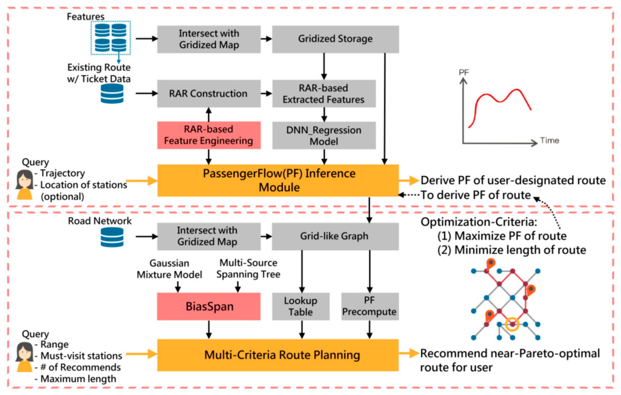
3.1. PF Inference Module

Given trajectories and stations of a certain arbitrary route, the goal of this module is to infer the PF (which refers to one of the criteria in our targeted route planning problem) for an arbitrary route given by the routing process in Section 4.

To be more precise, with the grid-based storage for heterogeneous urban data [85], the feature set for each existing route, including points of interest (POIs), entropy of POIs representing the diversity of urban functionalities [89], quantified relationships with existing mass-transit network, route network structure, and population structure, are extracted and integrated as training data. Accordingly, the corresponding ticket data is solicited and set as the training target, which refers to the PF under a certain timestamp. We employ DNN for regression as the inference model with various features treated as the inputs, and the PF values regarded as predictive labels [9]. Meanwhile, a pretrained model is adopted to infer the PF value of a given arbitrary route, which is generated by a route-planning algorithm, once this arbitrary route is deployed in the existing in-operation system.

3.2. Variable Desrcription

The description for variables defined in the problem formulation is listed in

Table 1. Description for variables defined in the problem formulation.

Variable	Description	Variable	Description
A	A range for planning.	F( )	The cost matrix associated with the edge.
G	A weighted, directed grid-like graph.	PF( )	The PF (profit) matrix associated with the route.
E	A set of edges (trajectories).	S	The set of stations.
EA	The set of edges located in area A.	SM	The set of must-visit stations.
eij	The edge-connecting node i and node j.	SMi	The must-visit station numbered i.
V	A set of nodes (grids).	SR	The set of recommended stations.
VA	The set of nodes located in area A.	SRi	The recommended station numbered i.
vi	The node i.	R	The number of recommended stations.
V’	A set of nodes (grids) as station candidates.	L	The maximum length for the route.
R	A route composed of stations and edges.

. It is worth mentioning that, the terms “edge” and “trajectory”, as well as “node (vertex)” and “grid” are interchangeable though depending on the scenario (e.g., real-world in-operation transit network, constructed grid-like graph) in some cases.

4. Multicriteria Route Planning for Mass Transit

4.1. Problem Formulation

We adopt and modify the grid-like graph as a weighted directed graph G = (V,E), in which V is the set of n nodes (grids) and E refers to the set of edges (trajectories). We set F = (f_ij) as the cost matrix associated with E, F corresponds to length (fuel consumption, or construction cost), and a route R in consist of V and E in the targeted problem. Another matrix associated with the selected trajectories E′ and stations V′ is route R′ = ({E′},{V′}) with PF(R), which refers to the expected PF of a temporary route R′ derived from the PF inference module. The PF is neither superimposable nor monotonic between routes; specifically, both PF and relative input features for the inference model are not monotonic. That is, a reinference is mandatory to retrieve an accurate PF of a route.

Precisely, our targeted problem is defined as follows. Given constraints consisting of (1) range for planning A (2) a set of must-visit stations S_M = {S_M0, …, S_Mi} (3) number of recommended stations r (4) maximum length L, our goal is to recommend a trajectory in a designated area along with a set of stations S = S_M + S_R so as to retain the Pareto-optimal between (1) profit (the PF value to be maximized, referring to the social welfare for the public) and (2) cost (the cost for construction and maintenance of the route to be minimized. The cost is positively correlated to the length of the route, referring to the sustainability for the government), in which S_M refers to the set of must-visit stations that shall be settled as the stations and included in the final route, S_R is the recommended stations {S_R0, …, S_Rr} that shall be derived by the given algorithm and included in the final route. Meanwhile, the Pareto-optimal here indicates that one method is able to retain the solutions under certain constraints (i.e., area size, or number of stations) if no other method has better performance in both objectives (‘profit’ and ‘cost’). For instance, given certain constraint (scenario), if two methods have the better performance in either of the two objectives against each other, and no other method has better performance (or could be called as the “improved satisfaction”) over these two methods in both objectives, then these two methods are both defined to reach the Pareto-optimal under this given scenario.

Precisely, the targeted problem can be formulated in the following equations:

$$\left\{\begin{array}{c}\mathrm{Maximize} \mathrm{PF}\left(\left\{{\displaystyle \sum }_{e_{ij}\in R}{e}_{ij}\right\},\left\{{\displaystyle \sum }_{v_i\in R}{v}_i\right\}\right).\\ \mathrm{Minimize} {\displaystyle \sum }_{e_{ij}\in R}\mathrm{F}\left(e_{ij}\right) \end{array}\right.$$

(1)

s.t.

$${{\displaystyle \sum }}_{e_{ij}\in R}\mathrm{F}\left(e_{ij}\right)\le L$$

(2)

$$E^{\prime }\subset E_A, V^{\prime }\subset V_A, R\subset A with R=\left(\left\{E’\right\},\left\{V’\right\}\right)$$

(3)

$$S\subset V\prime$$

(4)

$$S=S_M+S_R$$

(5)

$$S_{M_i}\subset V^{\prime } \forall S_M$$

(6)

$$S_{R_i}\subset V^{\prime } \forall S_R$$

(7)

$$S_{R_i}\not\subset S_{M_i} \forall S_R,S_M$$

(8)

$$S_{R_i}\subset V_A \forall S_R$$

(9)

$$S_{R_i}\not\subset \varnothing \forall S_R$$

(10)

$$\left|S_R\right|=r$$

(11)

$$V_A=V\cap A$$

(12)

$$E_A=E\cap A$$

(13)

in which R refers to the final route and consists of successive stations along with trajectories. Furthermore, Equation (1) refers to the optimization objectives, including the profit under queried constraints (the expected passenger flow to be maximized, referring to the social welfare for the public) and cost for construction as well as maintenance (the cost of route to be minimized, referring to the sustainability for the government). Furthermore, Equation (2) indicates that the length of the route shall not exceed the requested maximum length. While Equation (3) ensures the legal formulation of the final route been included in the queried planning area. Accordingly, Equations (4) and (5) defines the relationship between the vertices V′ in the final route and deployed stations S, as well as the deployed stations S and must-visit stations S_M with recommended stations S_R. Next, Equation (6) requires that all the must-visit stations shall be connected in the final route R’ (the trajectories E′ and the stations V′ in R′). Similarly, Equation (7) asks all the additional requested stations to be connected in the final route. Meanwhile, Equations (8)–(11) require the queried number of additional stations to be reached for further planning; furthermore, these additional stations shall be deployed in the delimited area without overlapping the vertices occupied by the must-visit stations. Accordingly, Equations (12) and (13) limit all the vertices and edges selected to be considered for route planning to be located in the requested area for planning.

4.2. The Strategy in BiasSpan

Due to the large number of possible combinations of trajectories and stations for constituting a route, the optimal solution turns out to be difficult to obtain, especially for large urban space. Precisely, according to our experiments, the exhaustion-based method is not feasible due to the long runtime. Furthermore, the targeted problem ends up being NP-Complete in attribution to the nonmonotonicity of input features and the uncertainty as a result of a heuristic function derived from PF. That is, due to the complexity in computational resource and nonmonotonic nature of the data, adequate modifications are needed for most heuristic algorithms to be eligible for solving the targeted problem [90]. Consequently, the Multi-source Bidirectional Gaussian-Prioritized Spanning Tree (BiasSpan) is proposed so as to obtain a decent solution in a reasonable time frame. The concepts of BiasSpan, which are inspired by the concept of parallel computing in bidirectional search as well as the goal-prioritization in best-first search, are composed of four parts, including grid-like graph construction, PF precomputation with lookup table construction, multisource bidirectional spanning, and the Gaussian mixture model for modelling spatial influence.

4.2.1. Grid-like Graph Construction

The BiasSpan algorithm relies on the grid-like graph for generating possible routes. The benefits are two-fold. First, the number of nodes can be significantly reduced since only some of the grids contain road segments. Using Chicago and Tainan as examples, based on the two cities’ road networks, the number of nodes in the two cities can be reduced from 390,509 and 237,866 to 91,320 and 94,282, respectively. To be more specific, since routes are confined to existing roads only, grids that contain no existing road network (299,189 and 143,584 grids for the two cities, respectively, contain features but do not correspond to existing roads) will not be considered for further trajectory construction. It is worth mentioning that the features stored in “no road” grids can still be fetched by indexing, since they still contribute to the PF inference of some routes. Second, when extracting features in RAR for a given route, the computational load and the time needed can be reduced by grid indexing.

4.2.2. PF Precomputation with Lookup Table Construction

The second strategy in BiasSpan lies in the precomputation that decreases the time consumption when accessing duplicate information. Precisely, the PF value for each grid in the map area is inferred and stored. Meanwhile, the edge weights (length) do not need to be stored as the distance between each adjacent grid is either 0.1 km or 0.1√2 km.

4.2.3. Multisource Bidirectional Spanning

Acting as a traditional yet efficient approach for limiting the searching space of path planning algorithm, BiasSpan employs multiple queues to be grown from each source (station) for bidirectional spanning. Accordingly, two queues are merged once their frontiers meet each other at certain grid, and the merged queue will then serve as the trajectory that connects their two corresponding sources. It is worth mentioning that a constraint where one source can only connect to a certain number of sources is activated in order to prevent the algorithm from constructing a radial route.

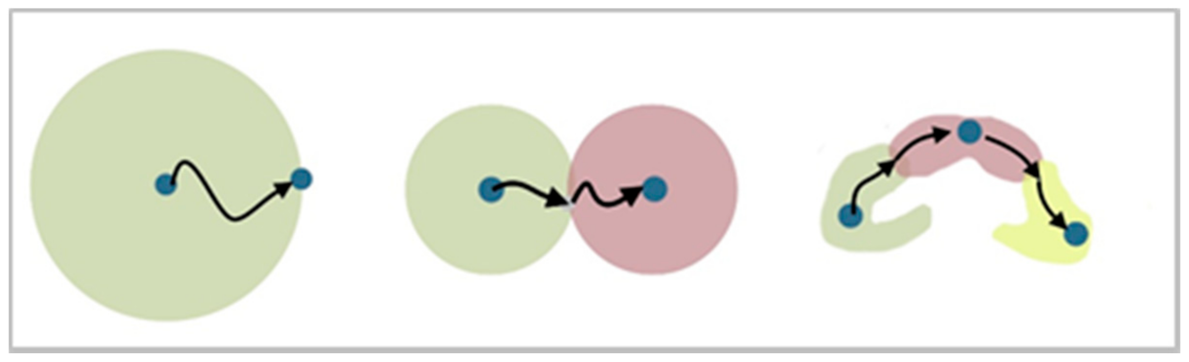
4.2.4. Gaussian Mixture Model for Modelling Spatial Influence

The Gaussian mixture model (GMM) is adopted for two main reasons, the countermeasure against herding effect in station deployment and the spatial influence of each station in the route-planning process. Precisely, for the first statement in the station deploying stage, if one only settles the recommended stations at locations with high potential PF, it could easily end up with a region where several stations are allocated. Therefore, the concept for applying GMM is that it enables the recomputation of PF considering the negative effects from regions (grids) where stations are already recommended. Additionally, such iterative process makes the stations suggested by BiasSpan not only based on high inferred PF of the grid itself, but also kept a distance from each other. Similarly, for the second statement in the route-planning stage, the spatial appeal for PF from each station, including must-visit ones and recommended ones, can be modelled by the two-dimensional GMM. In this way, not only the nonmonotonicity in each grid under urban space could be smoothed and thereafter the inaccuracy due to the uncertainty could be eased, but the goal-prioritization characteristic could also enhance the searching efficiency.

4.3. The Algorithm

Algorithm 1 to 3 depicts the pseudocode of each stage in the proposed BiasSpan: grid-preprocessing, station-recommending, and trajectory-routing. Where pf(g) refers to the inferred PF of grid g, G(g′,g) indicates the GMM function between grid g and g′, with gd(g′,g) showing the spatial distributed PF from grid g.

To be more precise, for the first part referring to Algorithm 1, the PF is retrieved for each must-visit station based on the pretrained DNN-based inference model mentioned in Section 3.1. Then the spatial appeal, or the spatial influence, of each station is evaluated for all the other grids based on the GMM. Meanwhile, the variance setting of Gaussian distribution refers to the grid size. Next, for Algorithm 2, the grid with maximal PF is iteratively selected as the recommended station based on the distributed PFs of GMM that neutralize the herding effect. Finally, for the third part (as described in Algorithm 3), the BiasSpan first limits the breadth of searching space based on GMM as described in Section 4.2.4; on the other hand, it decreases the depth of search in the spanning tree by the multisource bidirectional technique. BiasSpan ends up being a target-prioritized breadth-first spanning tree with multiple sources growing simultaneously.

Algorithm 1: Grid-Preprocessing for BiasSpan

input: grids and must_visit_grids (stations) in map area     Proposed PF inference model pf( )     output: Table gd( ) and tgd( )

foreach grid in area do     /*assign grid PF based on proposed inference model*/     let pf(grid) be the PF of grid     if grid is in must_visit_grids then     /*assign weights to nodes based on Gaussian-Distributed PF*/     foreach g in area do     let G(g, grid) be Gaussian function in 2 dimension     gd(g, grid) ← G(g, grid) × pf(grid)     tgd(g) ← tgd(g) + gd(g, grid)

Algorithm 2: Station-Recommending for BiasSpan

input: grids and must_visit_grids (stations) in map area Gaussian-Distributed PF gd( ) and accumulated GD-PF tgd( ) Proposed PF inference model pf( ) Given number_of_recommendedation output: Set recommended_grids

foreach j from 0 to number_of_recommendation do max(j) ← 0 choice ← null /*search maximum grid PF with accumulated GD-PF feedback*/ foreach g in area do if g is not in (must_visit_grids + recommended_grids) then if pf(g) − tgd(g) > max(j) then max(j) ← pf(g) − tgd(g) choice ← g add choice to recommended_grids /*assign weights to nodes based on Gaussian-Distributed PF*/ foreach g in area do let G(g, choice) be Gaussian function in 2 dimension gd(g, choice) ← G(g, choice) × pf(choice) tgd(g) ← tgd(g) + gd(g, choice)

Algorithm 3: Trajectory-Routing for BiasSpan

input: grids and must_visit_grids (stations) in map area road network (grid-like graph) Gaussian-Distributed PF gd( ) and accumulated GD-PF tgd( ) Set of recommended_grids output: route with starter as stations

starter ← must_visit_grids + recommended_grids /*initial the root, set and counter for each selected station*/ foreach grid in area do sid(grid) ← −1 if grid is in starter then root[starter_id] ← grid set[starter_id, 0].add(root[starter_id]) sid(grid) ← starter_id count(starter_id) ← 0 /*renew accumulated GD-PF based on negative feedback*/ foreach g in area do tgd[starter_id,0](g) ← tgd(g) − 2 × gd(g, grid) route ← null /*iterates until route is formed, restriction relaxes if fail*/ foreach i from 0 to infinite do /*each starter marches only one step in each iteration*/ foreach s in starter do /*there are multiple spanning trees for each starter*/ foreach st in set[s, i] do /*one starter meets at most 2 other starters*/ if count(s) ≥ 2 then break nst ← st/*deep copy*/ pt(nst, s) ← 0 max(st) ← 0 choice ← null /*search best direction among reachable & legal grids*/ foreach g in nearby_grid do if reachable in road network and sid(g) = s then renew relative parameters if current path is better if reachable in road network and sid(g) ≠ s then if tgd[s, i](g) > max(st) then max(st) ← tgd[s, i](g) choice ← g if choice ≠ null then nst.visit(choice) /*add to route if meets segment from other starter*/ if sid(g) ≠ −1 and count(sid(g)) < 2 then route.addseg(nst, obj(g)) count(s) ← count(s) + 1 count(sid(g)) ← count(sid(g)) + 1 if success to form a route with all starters then break /*accumulated GD-PF on negative feedback*/ foreach g in area do tgd[s,i](g)←tgd[s,i](g) − 2 × gd(g,root[sid(g)]) if count(sid(g)) = 2/*same for count(s) = 2*/then foreach st in starter do foreach g in area do tgd[st,i](g)←tgd[st,i](g) − 2 × gd(g,root[sid(g)]) else set[s, i + 1].add(nst) sid(g) ← s obj(g) ← nst pt(st, s) ← pt(st, s) + 1 /*each spanning tree tries at most 2 directions*/ if pt(st, s) > 1 then set[s, i].delete(st) set[s, i + 1].add(set[s, i]) tgd[s, i + 1] ← tgd[s, i] if success to form a route with all starters then break return route and starter

4.4. Summary of the Properties of BiasSpan

• BiasSpan employs GMM to deal with nonmonotonic gain function;
• The size of problem space for the algorithm is reduced based on the grid-like graph;
• BiasSpan prunes the searching space with a bidirectional goal-prioritized technique;
• The herding effect (crowding-out effect) in station recommendation is neutralized by the adopted GMM with negative feedback.

Apparently, there is no optimal solution to this multicriteria problem due to the trade-off between PF and length. Nonetheless, solutions are still expected to be provided by our proposed BiasSpan in a Pareto-optimal sense. Additionally, it is worth noting that although the implementation and the evaluation of the proposed BiasSpan are based on the constrained route planning for buses, where a new bus route is constrained by an existing road network and its revenue comes from fixed fares, this algorithm is still applicable for other types of mass transit. For instance, when applied to railroads, which are usually located underground but need to avoid existing pipes, a grid-like graph that avoids existing pipes and considers multiple layers could be constructed. Therefore, an unwanted collision could be prevented. Meanwhile, features needed to be considered, e.g., transference between existing routes, can still be stored in a grid-like graph for further inference.

4.5. Time Complexity

The targeted multicriteria nonmonotonic constrained route planning problem can be first simplified as a multiple-choice branching problem to explore its time complexity. The multiple-choice branching problem is defined to search for a subset A’∈A in a directed graph G = (V,A) with a partition of A into disjoint sets A₁, A₂, …, A_m. Meanwhile, the sum of weights in subset A′ is larger than a given positive integer K, so that A′ contains no cycles and at most one arc from each partition. Next, the “multiple choice branching” problem can be reduced into a 3-SAT problem, ends up being NP-Complete [91,92]. Furthermore, given that G is a strongly connected graph, it still remains NP-Complete since such a maximum weight branching problem can be viewed as a two-matroid intersection problem [93].

For the trajectory-routing part in BiasSpan, the time complexity turns out to be O(EV) given that the worst-case scenario is to traverse each grid in all directions. Where E is the number of maximum directions from one spanning tree (this variable is set to 2 in Algorithm 3, which equals to branching factor in the worst-case scenario), and V corresponds to the number of grids labelled in the searching area. For other routing algorithms introduced in previous sections, despite most of them turning out to be inapplicable towards solving this research problem or retrieving optimal solutions, the time complexity for brute-force searching is O(E^V), Dijkstra’s algorithm and Prim’s algorithm for O(EVlogV) or O(EV + VlogV), A* algorithm for O(E^V), and bidirectional search for O(SEV/S). Where S is the total number of stations, and E indicates the branching factor. It is worth noting that since V is far larger than S as well as E in most cases, BiasSpan is expected to find approximate solutions in a reasonable time among all the listed algorithms.

The schematic search space of different algorithms including the Dijkstra’s algorithm [94], bidirectional search, and BiasSpan is illustrated and compared in Figure 2. Based on the target-prioritized technique based on GMM, BiasSpan is expected to visit fewer candidates compared to bidirectional search.

5. Evaluation

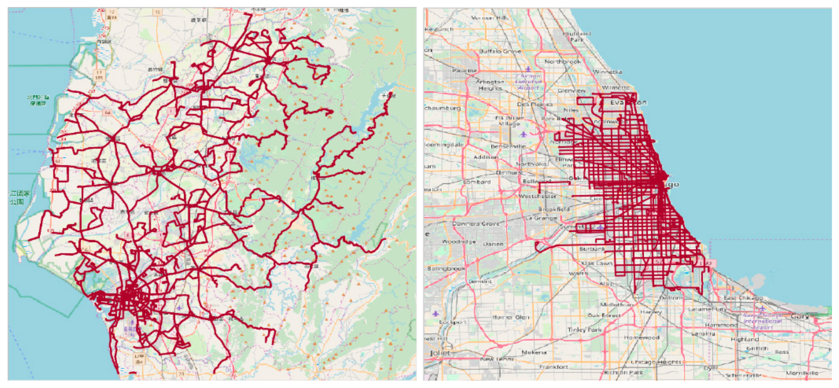
5.1. Dataset and Preprocessing

Two contrasting types (radial and square structure) of in-operation mass-transit networks retrieved from Tainan City Government and Chicago Transit Authority (CTA) are selected as the datasets for evaluation. As we introduced in previous sections, the proposed method is applicable for solving a multicriteria constrained planning problem towards various types of mass-transit systems. For evaluation, the bus-ticket data for Tainan lists the ticket ID, route ID, timestamps, and the starting and ending stations; on the other hand, the transit-ticket data for Chicago records the route ID, timestamps, and the number of passengers. Meanwhile, with 14,336,226 and 231,196,847 ticket records, respectively, for the mass-transit in these two cities, they both hold at least 100 routes and thousands of stations in service. Accordingly, the in-operation mass-transit networks for these two cities under the same scale are shown in Figure 3.

Next, as introduced in Section 3.1, heterogeneous urban information is harvested for constituting the input feature set in the PF inference module. To extract the necessary information, the POI is extracted from the GoogleMap, the road network structure with transportation hierarchy is loaded from the OpenStreetMap, and the population pyramid is fetched from respective agencies. Apart from the static features, the human mobility is represented by the bicycle and taxi record that lists both pick-up and drop-off locations. The size figure for the input instances of the two cities are listed in

Table 2. Size figures for our input instances.

Instance\Dataset		Tainan	Chicago
Bus data	Existing routes	104	139
	Existing stations	6575	11,592
	Ticket records	14,336,226	231,196,847
	Period	1 January 2017–31 December 2017	1 November 2017–30 October 2018
Gridization	Grids (0.1 km × 0.1 km)	505,296	330,335
Features	POI	8734	21,889
	Bike trips (for human mobility)	139,478	N/A
	Taxi trips (for human mobility)	N/A	68,461,612
	Road nodes	237,866	390,509
	Road edges	414,409	560,810
	Census blocks (for population)	14,730	46,293

.

Meanwhile, the urban spaces of Tainan and Chicago are divided into 505,296 and 330,335 disjoint grids (0.1 km × 0.1 km) based on EPSG: 3857, where only 94,282 and 91,320 grids (vertices) would be considered in route recommendation. The ranges in both EPSG: 3857 and 4326 projection for grid-like graph of two cities are listed in

Table 3. Boundaries for the grid and grid-like graph in Tainan and Chicago.

City	Tainan		Chicago
Projection	EPSG:3857	EPSG:4326	EPSG:3857	EPSG:4326
Upper bound	2,685,908.464	23.4448777	5,173,573.713	42.08402107
Lower bound	2,616,308.464	22.8700296	5,106,973.713	41.63844856
Right bound	13,433,041.310	120.6710632	9,742,334.669	87.51688136
Left bound	13,360,441.310	120.0188863	9,791,934.669	87.96244574

. The number of grids in both cities are reduced from 72.36% to 81.34% compared to the road network structure in real world.

5.2. Evaluation Setting

Six route-planning algorithms are selected as the comparative methods to search from one must-visit station for another iteratively:

• Dijkstra’s Algorithm (Dijkstra’s) [94]—Dijkstra’s algorithm is performed to search from one must-visit station towards other stations, either a must-visit one or recommended one. The destination then turns out to be the origin of a searching process in the next round for the Dijkstra’s algorithm to look for another stations. As an iterative process, it terminates until a route that connects all stations exactly once is formed.
• Breadth-First Search (BFS)—BFS is applied to take turns beginning the searching process from each of the must-visit stations. During the searching process, BFS will iteratively explore the adjacent candidate until there is no candidate that can be reached. Accordingly, the route planning is terminated until BFS successfully visits all the stations at least once, where a linear route is constructed.
• Iterative Deepening Depth-First Search (IDDFS) [95]—IDDFS acts as a depth-limited version of deep-first search (DFS). Towards the route planning problem, IDDFS is adopted to search for stations iteratively and employed with an increasing value in the setting of depth limit. Precisely, the searching process terminates once IDDFS can reach the stopping criteria where a route with all stations connected is formed under any setting of depth limit.
• Best-First Search (Best-First)—similar to the concept of BFS towards the routing process, Best-First explores the adjacent candidate with the highest PF iteratively. As a somewhat greedy algorithm focusing on the local optimal, the searching process terminates until a legal route is suggested.
• Distance-Based A* (Distance-A*)—the A* algorithm [25] is adopted with a heuristic emphasizing the distance between the candidate grid and the destination.
• Passenger-Flow-Based A* (PF-A*)—similar to Distance-A*, the A* algorithm here is adopted with a heuristic that predicts the PF between the candidate grid and the destination based on the pre-trained PF inference module introduced in Section 3.1.
• Brute-Force (BF)—acting as a baseline method, BF systematically enumerates all possible combinations in the problem space, and then the solution that retains the Pareto optimal among all enumerated candidate solutions is retrieved.

In accordance with our optimization objectives, which refer to reaching the Pareto-optimal between the PF and the cost of route, the PF and the cost will be reported along with an index of “PF per unit length” (or “unit PF”). It is worth mentioning that this “unit PF” index is one of the evaluating criteria in mass-transit planning according to our interview with civil servants in the Tainan City Bureau of Transportation; however, this is not one of the formulated optimization objectives concerning the multicriteria characteristic of the targeted research problem. The evaluation is based on 1000 randomly generated testing cases under various user-constrained settings. All methods are implemented in Java with a single core of an Intel [email protected] with 16 GB of RAM. To accommodate real-world scenarios, queries executed for over 20 min are identified as failures.

5.3. Evaluation of BiasSpan against Comparative Methods

The BiasSpan and comparative route-planning algorithms are performed under different user-constrained settings, including various area ranges and the number of must-visit stations. In this section, PF and length for each method is divided by the corresponding value of BiasSpan into a “PF ratio” or “length ratio;” and the unit PF for each method is divided by the value of BiasSpan into a unit PF ratio. The optimization criteria, the unit PF ratio, and runtime among all the methods are then compared.

The Pareto-efficient frontier and solutions under different area ranges are illustrated in Figure 4. The evaluation results for the optimization criteria including PF and length of route are illustrated in Figure 5, Figure 6, Figure 7 and Figure 8 for Chicago and Tainan datasets respectively. The PF ratio, length ratio, unit PF ratio, and runtime by varying area range (Figure 5, Figure 6, Figure 9 and Figure 10) and the number of must-visit stations (Figure 7, Figure 8, Figure 11 and Figure 12) are then compared. Detailed performance for Brute-Force are not depicted in Figure 5, Figure 6, Figure 7 and Figure 8 since it can only obtain solutions for very small ranges (<1 km²). The overall performance is evaluated in mean and standard deviation of solutions derived by different methods under various constrained settings for

Table 4. Performance for unit PF (to be maximized), PF (to be maximized), length (to be minimized), and runtime in mean and standard deviation of solutions derived from each method under different datasets and area ranges (small for <10 km²; middle for 10~100 km²; large for >100 km²).

Instance\Method			BiasSpan	Dijkstrta’s	BFS	IDDFS	Best-First	Distance-A*	PF-A*
City	Area	Indicator
Chicago	Overall	Unit PF	0.25 ± 0.31	0.16 ± 0.24	0.09 ± 0.17	0.09 ± 0.18	0.08 ± 0.15	0.15 ± 0.23	0.10 ± 0.18
		PF	2.12 ± 3.36	2.67 ± 5.19	3.48 ± 7.61	3.38 ± 7.30	2.32 ± 4.05	2.74 ± 5.43	2.34 ± 4.11
		Length	15.10 ± 12.72	39.21 ± 44.55	98.37 ± 113.16	132.64 ± 183.12	92.09 ± 107.54	40.59 ± 45.98	82.48 ± 104.16
		Runtime	10.78 ± 30.46	198.06 ± 387.53	93.92 ± 120.88	9792.84 ± 3.0 × 104	158.74 ± 269.83	94.17 ± 155.97	271.98 ± 558.73
	Small	Unit PF	0.56 ± 0.39	0.36 ± 0.33	0.24 ± 0.26	0.26 ± 0.28	0.22 ± 0.23	0.36 ± 0.32	0.26 ± 0.27
		PF	0.91 ± 0.35	0.91 ± 0.35	0.91 ± 0.35	0.91 ± 0.35	0.91 ± 0.35	0.91 ± 0.35	0.91 ± 0.35
		Length	2.33 ± 1.44	5.14 ± 5.19	8.53 ± 7.88	8.18 ± 7.96	9.23 ± 9.52	5.17 ± 5.15	7.26 ± 7.13
		Runtime	1.50 ± 0.26	10.60 ± 3.74	10.09 ± 3.51	11.75 ± 5.06	11.02 ± 4.50	10.43 ± 3.77	10.91 ± 4.47
	Middle	Unit PF	0.16 ± 0.19	0.09 ± 0.14	0.04 ± 0.08	0.04 ± 0.06	0.03 ± 0.06	0.08 ± 0.12	0.04 ± 0.08
		PF	1.94 ± 2.60	2.28 ± 3.78	2.77 ± 5.36	2.74 ± 5.33	2.08 ± 3.09	2.29 ± 3.72	2.15 ± 3.32
		Length	14.22 ± 6.72	36.38 ± 28.14	88.56 ± 69.11	106.35 ± 87.45	94.72 ± 66.09	37.44 ± 28.44	80.01 ± 54.41
		Runtime	5.55 ± 3.45	88.34 ± 71.11	66.71 ± 40.85	1390.57 ± 2.1 × 103	101.87 ± 63.18	55.44 ± 36.19	141.23 ± 109.75
	Large	Unit PF	0.14 ± 0.21	0.09 ± 0.15	0.05 ± 0.08	0.04 ± 0.08	0.04 ± 0.06	0.08 ± 0.12	0.04 ± 0.06
		PF	4.28 ± 5.76	6.18 ± 9.15	9.05 ± 13.45	8.57 ± 12.74	4.89 ± 6.99	6.54 ± 9.81	4.85 ± 6.92
		Length	34.78 ± 10.84	93.14 ± 60.75	247.59 ± 143.38	377.47 ± 270.44	194.69 ± 169.58	97.24 ± 62.46	190.19 ± 168.51
		Runtime	38.85 ± 62.68	777.19 ± 606.13	287.31 ± 154.63	4.8 × 104 ± 5.6 × 104	526.29 ± 449.92	321.99 ± 245.04	1012.30 ± 968.80
Tainan	Overall	Unit PF	0.08 ± 0.15	0.05 ± 0.10	0.04 ± 0.09	0.03 ± 0.08	0.03 ± 0.09	0.04 ± 0.10	0.04 ± 0.09
		PF	0.25 ± 0.04	0.26 ± 0.06	0.26 ± 0.07	0.27 ± 0.08	0.25 ± 0.04	0.26 ± 0.06	0.25 ± 0.04
		Length	18.40 ± 18.95	47.03 ± 51.53	85.68 ± 96.02	122.39 ± 160.31	100.40 ± 114.80	49.01 ± 53.38	91.84 ± 107.23
		Runtime	7.57 ± 11.57	103.87 ± 172.85	74.98 ± 91.16	3625.33 ± 8.3 × 103	151.76 ± 233.04	77.46 ± 123.33	106.24 ± 137.43
	Small	Unit PF	0.24 ± 0.19	0.14 ± 0.14	0.12 ± 0.15	0.11 ± 0.12	0.10 ± 0.14	0.13 ± 0.14	0.11 ± 0.14
		PF	0.22 ± 2.8 × 10−3	0.22 ± 6.1 × 10−4	0.22 ± 6.1 × 10−4	0.22 ± 6.1 × 10−4	0.22 ± 6.1 × 10−4	0.23 ± 7.7 × 10−3	0.22 ± 6.1 × 10−4
		Length	1.92 ± 1.54	4.56 ± 4.90	7.11 ± 7.50	7.13 ± 8.55	8.14 ± 7.53	4.52 ± 3.92	6.60 ± 5.53
		Runtime	0.94 ± 0.51	4.68 ± 2.19	4.79 ± 2.71	7.44 ± 3.54	5.43 ± 3.23	4.96 ± 2.70	5.68 ± 3.41
	Middle	Unit PF	0.02 ± 0.01	0.01 ± 0.01	5.2 × 10−3 ± 3.7 × 10−3	3.6 × 10−3 ± 2.6 × 10−3	3.9 × 10−3 ± 3.2 × 10−3	8.0 × 10−3 ± 4.8 × 10−3	4.4 × 10−3 ± 3.8 × 10−3
		PF	0.25 ± 0.04	0.26 ± 0.05	0.27 ± 0.06	0.28 ± 0.07	0.26 ± 0.04	0.26 ± 0.05	0.26 ± 0.04
		Length	17.70 ± 8.25	48.64 ± 37.37	87.04 ± 71.63	117.40 ± 74.56	110.66 ± 70.85	48.27 ± 33.19	98.83 ± 66.85
		Runtime	4.95 ± 3.23	72.36 ± 57.11	62.19 ± 41.38	1294.13 ± 1.9 × 103	115.71 ± 64.87	50.62 ± 34.34	87.36 ± 46.36
	Large	Unit PF	7.1 × 10−3 ± 3.3 × 10−3	3.6 × 10−3 ± 2.3 × 10−3	2.1 × 10−3 ± 1.5 × 10−3	2.0 × 10−3 ± 1.8 × 10−3	2.4 × 10−3 ± 2.1 × 10−3	3.2 × 10−3 ± 2.1 × 10−3	2.4 × 10−3 ± 2.1 × 10−3
		PF	0.27 ± 0.05	0.29 ± 0.08	0.32 ± 0.10	0.33 ± 0.10	0.28 ± 0.06	0.30 ± 0.08	0.28 ± 0.06
		Length	47.95 ± 22.34	113.02 ± 58.71	212.53 ± 101.88	329.43 ± 252.49	223.36 ± 172.93	125.35 ± 60.73	212.93 ± 157.40
		Runtime	26.48 ± 16.60	363.74 ± 269.45	230.32 ± 95.46	1.7×104 ± 1.3×104	503.83 ± 362.70	278.79 ± 176.58	330.48 ± 179.88

, and in hypervolume (HV) of Pareto set obtained by different methods under various constrained settings for

Table 5. Hypervolume (HV) obtained by each method under different datasets and area ranges.

Instance\Method		BiasSpan	Dijkstrta’s	BFS	IDDFS	Best-First	Distance-A*	PF-A*
City	Area
Chicago	Overall	0.107014	0.088183	0.045771	0.067346	0.057848	0.066998	0.076158
	Small	0.436986	0.549837	0.404202	0.675657	0.367308	0.541177	0.452289
	Middle	0.624969	0.408880	0.302886	0.383707	0.343325	0.289418	0.475395
	Large	0.926956	0.663704	0.835865	0.636061	0.614135	0.464512	0.613291
Tainan	Overall	0.646061	0.493045	0.442171	0.443477	0.573544	0.485285	0.575067
	Small	0.997011	0.996559	0.995518	0.995249	0.995512	0.867559	0.995548
	Middle	0.866878	0.753219	0.672815	0.733803	0.785875	0.875773	0.782592
	Large	0.972058	0.819815	0.967445	0.863522	0.985707	0.895531	0.985480

. Additionally,

Table 6. Probability for BiasSpan to retrieve a better solution (higher unit PF, higher PF, shorter length) in all test cases compared to other methods.

Instance\Comparative		Dijkstrta’s	BFS	IDDFS	Best-First	Distance-A*	PF-A*
Chicago	Unit PF	76.25%	98.91%	97.66%	99.69%	78.59%	98.75%
	PF	57.19%	59.22%	60.16%	61.41%	56.56%	63.91%
	Length	77.03%	99.38%	98.28%	99.84%	79.53%	98.91%
Tainan	Unit PF	89.11%	100.00%	99.01%	100.00%	94.06%	100.00%
	PF	39.60%	36.63%	37.62%	51.49%	40.59%	47.52%
	Length	89.33%	100.00%	99.21%	100.00%	94.12%	100.00%

shows the probability for BiasSpan to retrieve a better solution compared to other methods.

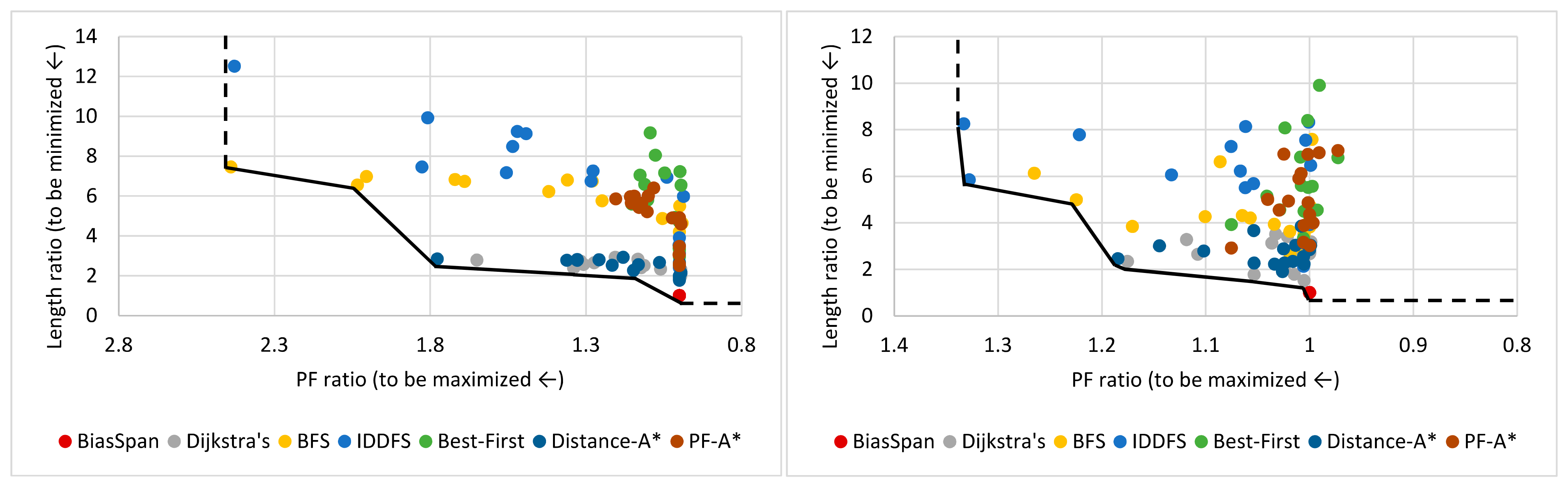
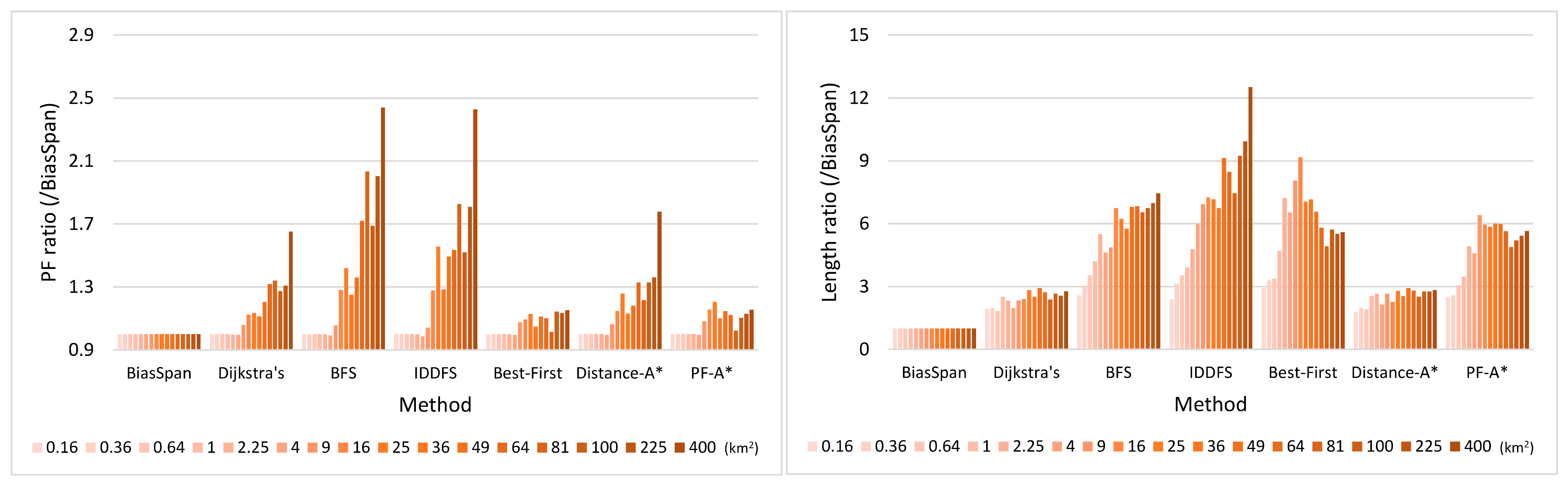
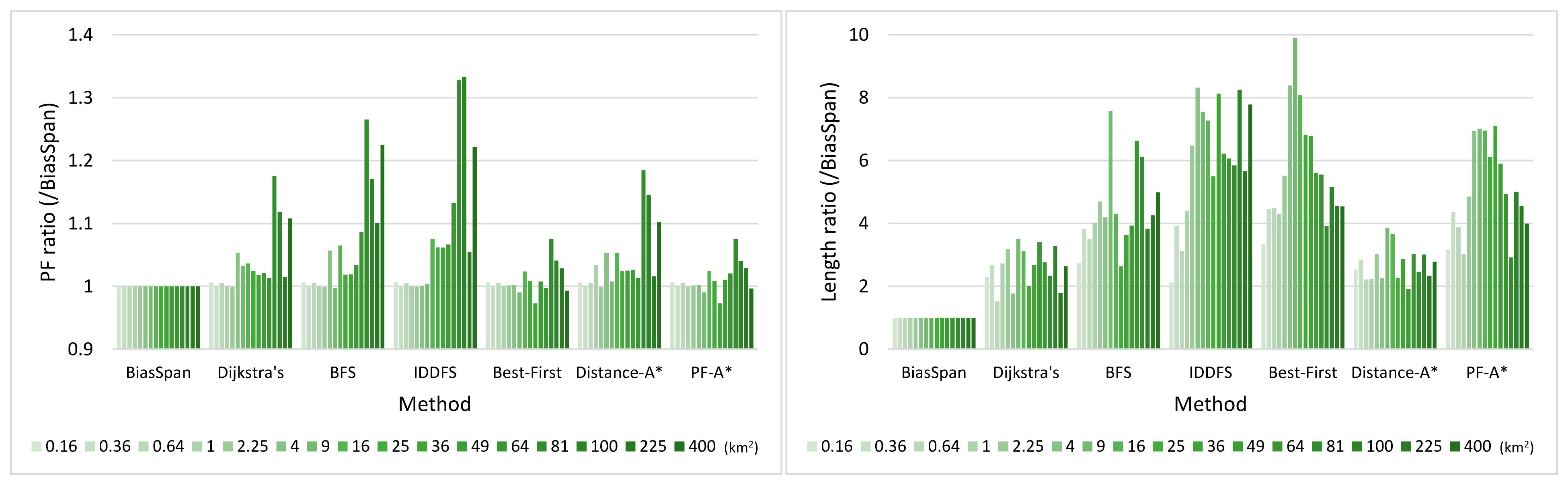
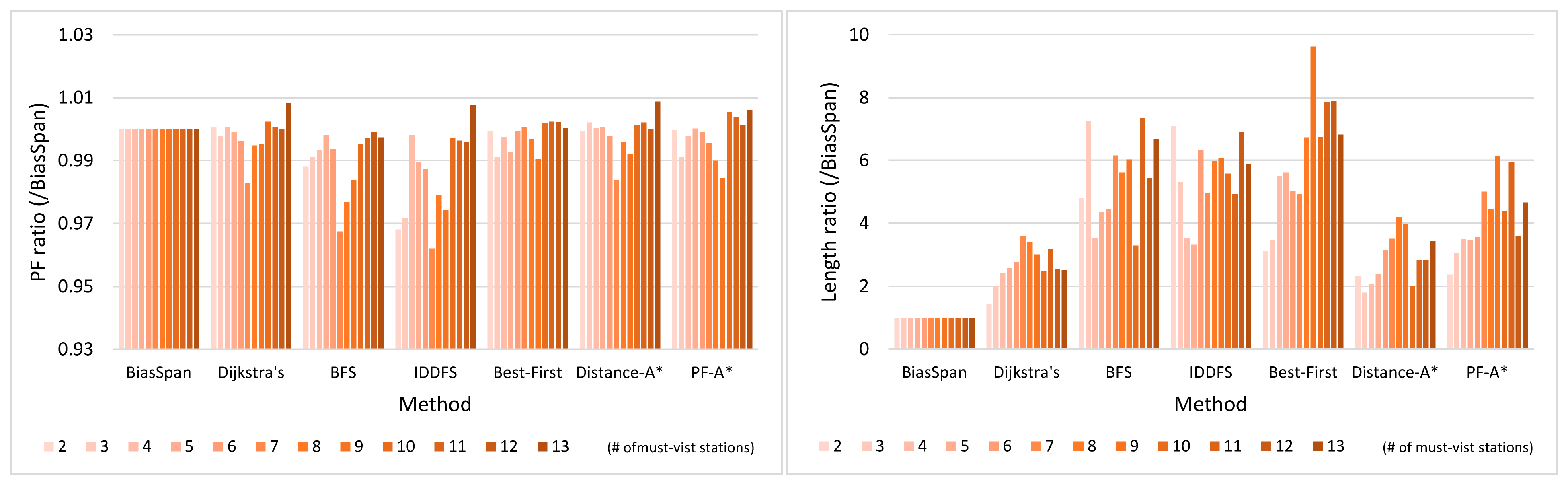
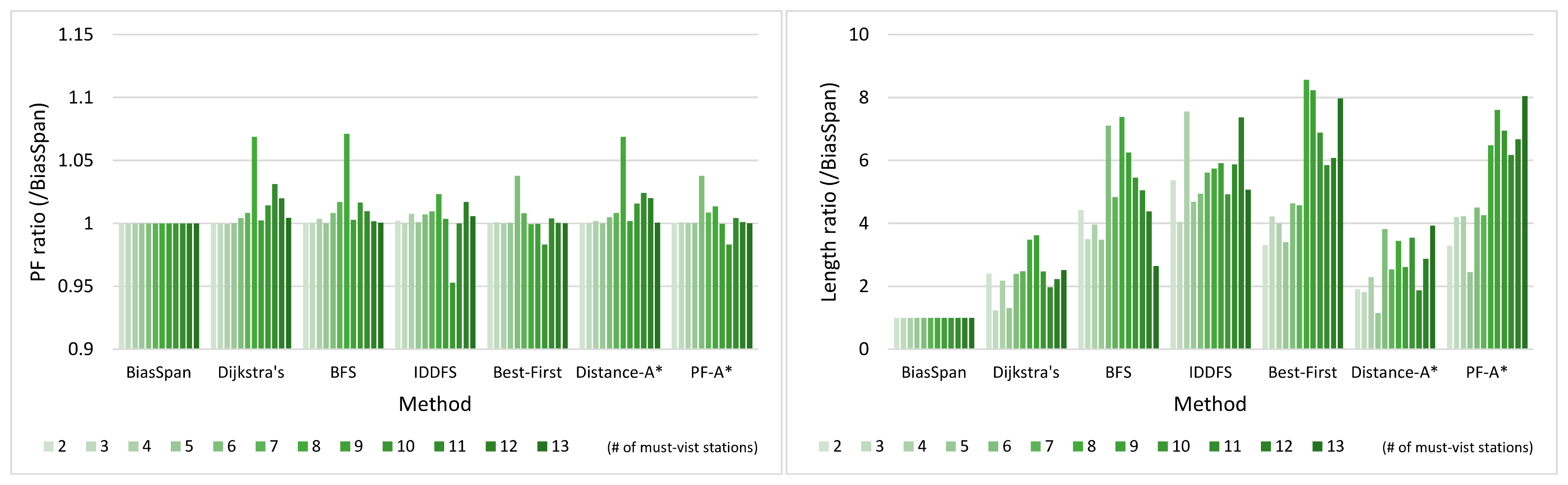
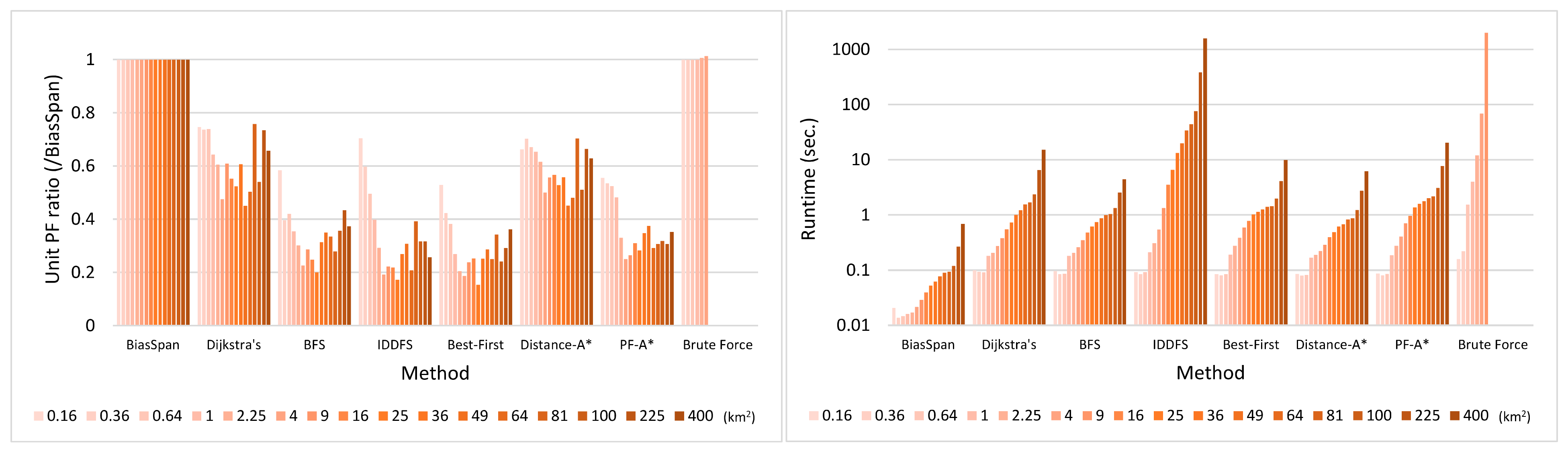
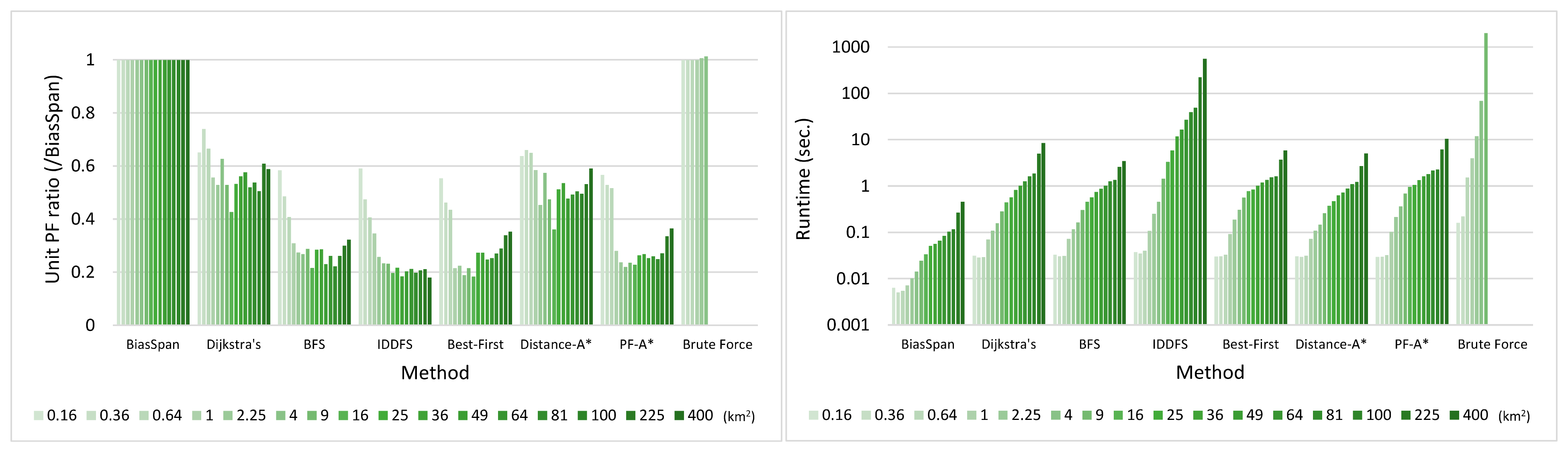
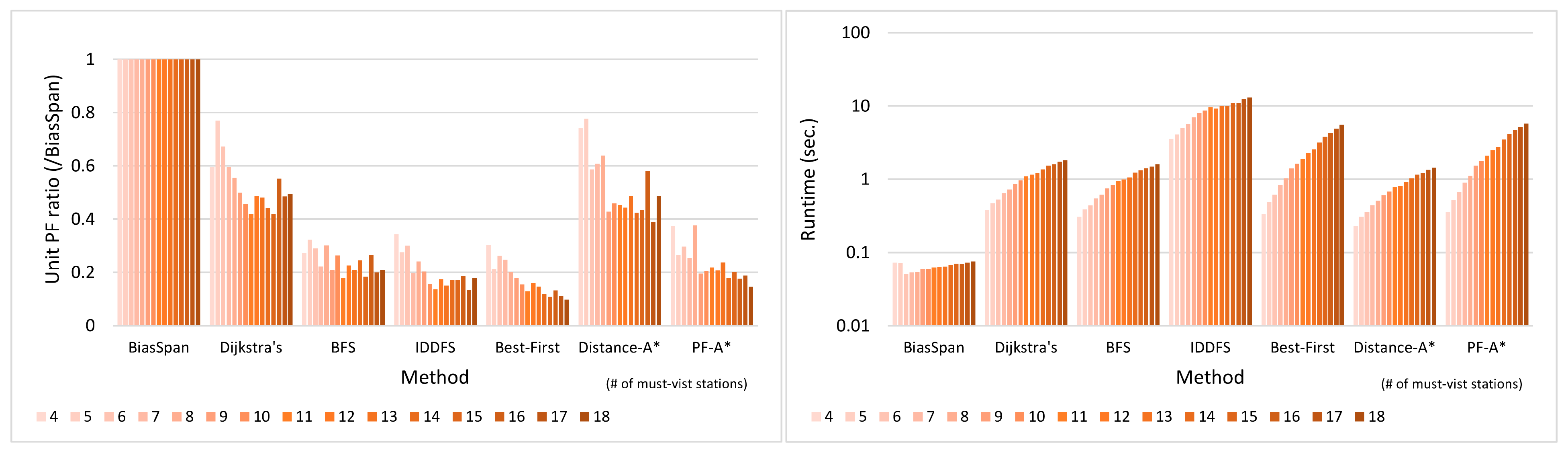
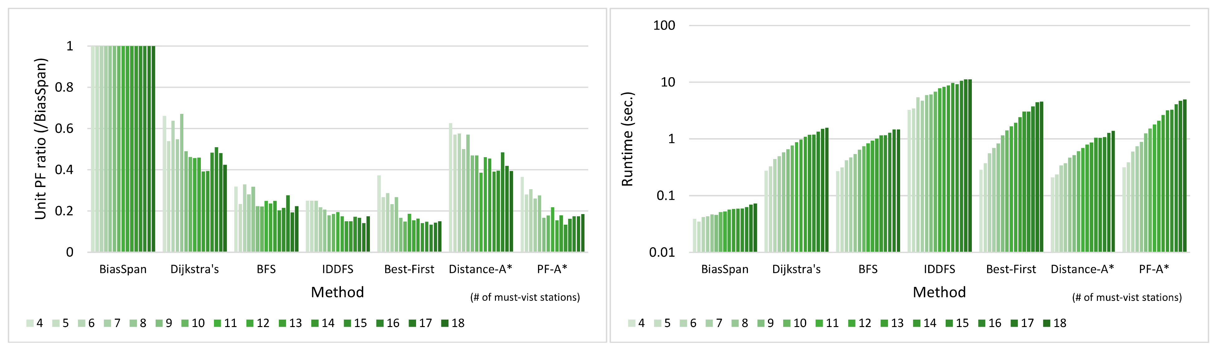
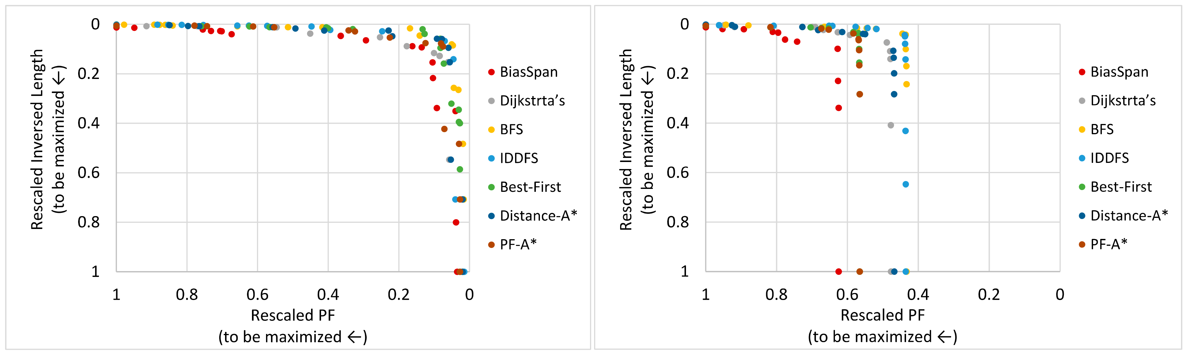
5.3.1. Pareto-Optimal between Profit and Cost

Overall experimental results indicate that BiasSpan maintains high PF per unit length and success rate in the middle-scale and large-scale region, where its length ratio referring to the cost of route outperforms that of other methods. First, we compare the length and corresponding PF of routes generated by different methods in Figure 5, Figure 6, Figure 7, Figure 8, Figure 9, Figure 10, Figure 11 and Figure 12. Although BiasSpan and other comparative methods gain similar performance for route length and especially the PF of route in small-scale region, the chasm takes place in a larger region, where the length for Distance-A* and Dijkstra’s is two to three times longer than the one for BiasSpan, and, at the same time, the value turns out to be around four to six for BFS, Best-First, and PF-A*. Finally, the length of the route generated by IDDFS is eight times longer than the one generated by BiasSpan. When a larger region is given, more than half of the queries of IDDFS cannot successfully generate a route in time.

As both Distance-A* and Dijkstra’s focus on retrieving a solution simply seeking the best performance in shortening the length of route, they turn out to ignore another objective in this multicriteria routing problem. Precisely, they indeed somewhat successfully suggest a trajectory that connects each pair of the stations with a lower cost compared to the other algorithms. Unfortunately, due to the nature of the iterative routing process where an adopted algorithm is conducted from station to station without proper serialization in the order of stations, these two methods, in the end, return a route with lower quality in the criterion of cost (length). For instance, given three or more stations during route construction, Distance-A* and Dijkstra’s algorithms may create a crooked or even zigzagging trajectory (e.g., hairpin shape or switchback) while trying to connect all these stations successively. In contrast, by adopting the multisource bidirectional spanning technique, BiasSpan is able to plan smooth, efficient routes with minimal turns and disruptions.

Meanwhile, since Best-First and PF-A* focus on the efficacy of PF, it seems that they both fail to address the length of the route and thereafter generate trajectories that connect and make several successive detours in small regions, especially in the areas with high potential PF. An intriguing result is that, despite their emphasis on the efficacy of PF, the evaluation shows that Best-First and PF-A* both end up with low overall PF performance compared to Distance-A* and Dijkstra’s. This may be attributed to the nonmonotonicity in heuristic as well as the heterogeneity in urban space. In short, the evaluation confirms that forming trajectories by simply integrating grids is definitely not a feasible approach.

5.3.2. Runtime

First of all, BiasSpan is able to responds to queries in the scale of 10⁻¹ to 10⁻² s in small- to middle-scale problem space. Meanwhile, the runtime of comparative methods are at least one logarithmic scale longer than the one of BiasSpan; among them, IDDFS holds the longest runtime apart from Brute-Force and is around two to three logarithmic scales longer than BiasSpan’s. This can be attributed to the nature of IDDFS, which is a DFS-based routing algorithm. In other words, compared BiasSpan or the other comparative methods, IDDFS could easily end up with exploring regions where no station exists. For other comparative methods, BFS, Best-First, and Distance-A* tend to consume less time compared to Dijkstra’s and PF-A* given the same problem space.

To be more explicit, experimental results on the runtime shown in Figure 9, Figure 10, Figure 11 and Figure 12 meet our estimate that, for BiasSpan, its time complexity is mainly related to the size of problem space. Meanwhile, BiasSpan holds a runtime that outperforms most of the comparative methods for at least one logarithmic scale and is close to Best-First Search and Distance-A*.

5.3.3. Trade-Off between Profit and Cost

Accordingly, BiasSpan sacrifices some PF to secure the length of route; to be more precise, this trade-off is valued considering the pessimism about the error as well as the uncertainty in PF. Since the PF itself is an inferred value with RMSE as described in previous evaluations, even if the route-planning algorithm retains a solution with an outstanding PF, the exact efficacy for the route (solution) been deployed in real-world scenario rather than in this ideal evaluation scenario is referable yet uncertain.

In contrast, the criterion of length of route turns out to be much more reliable since there is less error in the cost for construction, maintenance, and fuel consumption between real-world scenario and our evaluation. Nonetheless, the evaluation still demonstrates the adaptability of our proposed BiasSpan in overall performance and the ability to deal with the trade-off between PF and length of route.

Despite the discussion of reliability and error in objectives, the concept of the hypervolume (HV) is adopted to evaluate the performance of methods under the multicriteria scenario. As the calculation of HV asks for a reference point with its performance worse than the nadir point in the original Pareto set for all objectives [96], and to better exemplify the analysis, the nondominated solutions from all solutions retained by different methods are illustrated in Figure 13, where both objectives, PF and inversed length, are normalized and to be maximized. The (0, 0) is then selected as the reference point for calculating HV, which thereafter makes HV to be maximized. The HV obtained by each method is listed in Table 5, where BiasSpan secures the best HV for overall solutions in both datasets.

To be more precise, the HV obtained by BiasSpan compared to other methods shows an intriguing trend where BiasSpan has a better performance in middle-scale to large-scale problem spaces in the Chicago dataset, but only retains a better result in a small-scale problem space in the Tainan dataset. Furthermore, IDDFS seems to achieve the best performance in HV in small-scale problem space in Chicago; however, the advantages fall to the Distance-A* and PF-A* for the best solutions in middle-scale and large-scale Tainan dataset, respectively. This phenomenon may be attributed to the nature of road network in the two cities, where a square structure may enhance a balance exploration in both benefit and cost for the BiasSpan. Explicitly, the distribution of spatial influence in features can be more effectively delivered from the stations to other vertices in the graph through this certain formation of connectivity. Nonetheless, the evaluation results in HV proves that the BiasSpan is able to secure the Pareto optimal under the concerns in the nature of objective itself.

5.3.4. Statistical Analysis for BiasSpan

For the statistical analysis of BiasSpan against other comparative methods, the one-way analysis of variance (ANOVA), two-way ANOVA, Fisher’s least significant difference (LSD), and Wilcoxon signed-rank tests are adopted with a significance level of 0.05.

The results for two-way ANOVA test for different methods and constraints towards unit PF performance are listed in

Table 7. Two-way ANOVA test for different methods and constraints towards unit PF performance.

City	Source	DF	SS	MS	F-Value	p-Value
Chicago	Method	6	0.361537984	0.060256331	33.77470726	4.77 × 10−21
	Area	15	2.021735304	0.134782354	75.54782186	3.09 × 10−44
	Error	90	0.160566003	0.001784067
	Total	111	2.543839291
	Method	6	0.240735177	0.040122529	23.67341257	1.00 × 10−14
	Station	11	0.318606133	0.028964194	17.08968306	2.44 × 10−15
	Error	66	0.111859114	0.001694835
	Total	83	0.671200423
Tainan	Method	6	0.016672738	0.002778790	5.828486175	3.64 × 10−5
	Area	15	0.411747878	0.027449859	57.57582978	1.96 × 10−39
	Error	90	0.042908409	0.000476760
	Total	111	0.471329025
	Method	6	0.006929104	0.001154851	58.45235695	1.66 × 10−24
	Station	11	0.003567283	0.000324298	16.41425121	6.22 × 10−15
	Error	66	0.001303970	1.98 × 10−5
	Total	83	0.011800358

. Meanwhile, the p-values in two-way ANOVA test for different methods towards all objectives are depicted in

Table 8. p-Values in two-way ANOVA test for different methods towards all objectives.

City	Source	DF	Unit PF	PF	Length
Chicago	Method	6	4.77 × 10−21	3.27 × 10−5	2.10 × 10−10
	Area	15	3.09 × 10−44	1.11 × 10−35	1.10 × 10−17
	Method	6	1.00 × 10−14	1.48 × 10−7	2.46 × 10−17
	Station	11	2.44 × 10−15	7.34 × 10−80	5.45 × 10−13
Tainan	Method	6	3.64 × 10−5	1.56 × 10−6	1.43 × 10−12
	Area	15	1.96 × 10−39	6.48 × 10−43	2.13 × 10−23
	Method	6	1.66 × 10−24	0.07 × 10−2	3.50 × 10−16
	Station	11	6.22 × 10−15	1.11 × 10−34	3.34 × 10−10

. To be more specific, the two-way ANOVA is based on the fitness function of unit PF in Table 7, and all targeted criteria (PF, length, unit PF) for Table 8. As the p-values demonstrated, it seems that there is a significant difference between the solutions generated by various methods and under different constrained settings. This result first supports the complexity as well as heterogeneity of the problem space, where different formations of constrained settings indeed affect the constitutions and performance of the possible solutions. Furthermore, it seems that the solutions generated by different methods have different efficacy between each other based on the reported results.

To better interpret the different efficacies among various algorithms, the one-way ANOVA test is applied based on the unit PF performance and its results are depicted in

Table 9. One-way ANOVA test for different methods and constraints towards unit PF performance.

City	Source	DF	SS	MS	F-Value	p-Value
Chicago	Method	6	1.203675884	0.200612647	21.56892294	4.55 × 10−22
	Error	413	3.841314821	0.009301004
	Total	419	5.044990705
Tainan	Method	6	0.034645522	0.005774254	32.96143117	1.88 × 10−32
	Error	413	0.072350218	0.000175182
	Total	419	0.106995740

. Next, Fisher’s LSD test is applied to examine the cluster of different methods according to the performance towards unit PF. Based on the results of Fisher’s LSD test in

Table 10. Fisher’s LSD test based on one-way ANOVA.

City	LSD	Indicator	BiasSpan	Dijkstrta’s	BFS	IDDFS	Best-First	Distance-A*	PF-A*
Chicago	0.03461	Mean	0.25280	0.15798	0.09373	0.09114	0.08128	0.15277	0.09747
		Std.	0.31434	0.23687	0.16829	0.17891	0.14793	0.22618	0.17577
		Grouping	A	B	C	C	C	B	C
Tainan	0.00475	Mean	0.08129	0.04597	0.03702	0.03378	0.03255	0.04262	0.03597
		Std.	0.14666	0.09651	0.09355	0.07890	0.08870	0.09504	0.09162
		Grouping	A	B	C	D	D	B	C

, it seems that the unit PF obtained from BiasSpan is significantly better than those retrieved from other comparative methods. In other words, based on the fitness function of unit PF, BiasSpan is clustered on its own in the first-tier group for its performance in both datasets. On the other hand, Dijsktra’s and Distance-A* are both clustered in the second-tier group for their performance in both datasets, while IDDFS and Best-First are clustered in the last-tier group for both datasets. For the rest methods, BFS and PF-A* turns out vary between the second tier and last tier depending on the datasets. This can be credited to the stability of effective exploration in grids for the route-planning algorithm itself. For instance, the decisions made by Dijsktra’s and Distance-A* tend to be attracted by the expected minimized cost in length, which seems to be a more reliable and less nonmonotonic feature compared to the other criterion. In contrast, IDDFS and Best-First aim to retain a better estimated profit in PF; however, they risk falling into local optimal or failing to secure a smooth path, which, in turn, leads these two methods together a worse performance. Similarly, the characteristics of BFS and PF-A* also put some emphasis in searching for local optimal in the profit of PF, yet the cost is still considered in their mixed nature. This makes them fall in between these two types and end up with a mediocre position among all the tested algorithms.

To further investigate the performance BiasSpan, the Wilcoxon signed-rank test for BiasSpan against other comparative methods towards all objectives is conducted with the results listed in

Table 11. Wilcoxon signed-rank test for BiasSpan against different methods towards all objectives.

City	Objective	Indicator	Dijkstra	BFS	IDDFS	Best-First	Distance-A*	PF-A*
Chicago	Unit PF	p-value	6.07 × 10−6	8.67 × 10−19	8.67 × 10−19	8.67 × 10−19	2.60 × 10−9	8.67 × 10−19
		Positive ranks	47	60	60	60	52	60
		Negative ranks	13	0	0	0	8	0
	PF	p-value	0.1225	0.0031	0.0067	0.0259	0.1831	0.0462
		Positive ranks	35	41	40	38	34	37
		Negative ranks	24	19	20	22	25	23
	Length	p-value	6.07 × 10−6	8.67 × 10−19	8.67 × 10−19	8.67 × 10−19	2.60 × 10−9	8.67 × 10−19
		Positive ranks	13	0	0	0	8	0
		Negative ranks	47	60	60	60	52	60
Tainan	Unit PF	p-value	0.0031	8.67 × 10−19	8.67 × 10−19	8.67 × 10−19	8.08 × 10−8	8.67 × 10−19
		Positive ranks	41	60	60	60	50	60
		Negative ranks	18	0	0	0	10	0
	PF	p-value	0.2595	0.0005	0.0259	0.0259	0.0775	0.0031
		Positive ranks	27	17	22	22	24	19
		Negative ranks	29	41	36	36	33	39
	Length	p-value	0.0031	8.67 × 10−19	8.67 × 10−19	8.67 × 10−19	8.08 × 10−8	8.67 × 10−19
		Positive ranks	18	0	0	0	10	0
		Negative ranks	41	60	60	60	50	60

. As a non-parametric alternative to the paired t-test, it shows that for the objective of length of fitness function (unit PF), BiasSpan turns out to retain significantly better performance compared to all other methods in both datasets. It is worth mentioning that, since the objective of length is to be minimized, a larger amount of negative ranks indicates that BiasSpan obtains a solution with better performance in the criterion of length against its competitor. Although comparative methods such as BFS and PF-A* tend to retrieve a better performance in the objective of PF, especially in the Tainan dataset, the disadvantage is not that not significant according to the significance level as well as compared to its advantage in the other objective.

Meanwhile, despite the discussion of BiasSpan against other comparative methods, the p-values in Wilcoxon signed-rank test for all pairs of methods towards unit PF performance are shown in

Table 12. p-Values in Wilcoxon signed-rank test for all pairs of methods towards unit PF performance. Where “N.A.” refers to incompatibility since the algorithm cannot be compared to itself; and “D.A.” refers to the disadvantage where the targeted method has more negative ranks than positive ranks when been analyzed with the comparative method.

City	Method	Comparative Method
		BiasSpan	Dijkstra	BFS	IDDFS	Best-First	Distance-A*	PF-A*
Chicago	BiasSpan	N.A.	6.07× 10−6	8.67× 10−19	8.67× 10−19	8.67× 10−19	2.60× 10−9	8.67× 10−19
	Dijkstra	D.A.	N.A.	4.86 × 10−11	1.54 × 10−8	1.54 × 10−8	1.59 × 10−6	6.73 × 10−5
	BFS	D.A.	D.A.	N.A.	0.5513	0.4487	D.A.	D.A.
	IDDFS	D.A.	D.A.	D.A.	N.A.	0.0775	D.A.	D.A.
	BestFirst	D.A.	D.A.	D.A.	D.A.	N.A.	D.A.	D.A.
	Distance-A*	D.A.	D.A.	3.84 × 10−10	1.54 × 10−8	6.07 × 10−6	N.A.	0.0002
	PF-A*	D.A.	D.A.	0.0067	0.0259	0.0002	D.A.	N.A.
Tainan	BiasSpan	N.A.	0.0031	8.67× 10−19	8.67× 10−19	8.67× 10−19	8.08× 10−8	8.67× 10−19
	Dijkstra	D.A.	N.A.	5.19 × 10−12	4.54 × 10−13	5.19 × 10−12	0.0005	2.60 × 10−9
	BFS	D.A.	D.A.	N.A.	0.0259	0.3494	D.A.	0.1225
	IDDFS	D.A.	D.A.	D.A.	N.A.	D.A.	D.A.	D.A.
	BestFirst	D.A.	D.A.	D.A.	0.0462	N.A.	D.A.	D.A.
	Distance-A*	D.A.	D.A.	1.54 × 10−8	1.59 × 10−6	8.08 × 10−8	N.A.	8.08 × 10−8
	PF-A*	D.A.	D.A.	D.A.	0.1225	0.0031	D.A.	N.A.

, in which the disadvantage where the targeted method has more negative ranks than positive ranks against comparative methods is noted as “D.A.”. This demonstrates a similar result to the Fisher’s LSD test recorded in Table 10; nonetheless, there are some differences between these two somewhat clustering results. Precisely, BiasSpan still holds a performance significantly outperforming other competitors; while Dijsktra’s and Distance-A* are still grouped in the second tier, though Dijsktra’s secures better results. The discrepancy seems to lie in the PF-A*. It seems that Dijsktra’s significantly surpasses PF-A* especially in Tainan dataset, for which Dijsktra’s and PF-A* are clustered in the middle tiers as listed in Table 10. Indeed, there is no significant difference among the unit PF performance achieved by BFS, PF-A*, IDDFS, and Best-First, though PF-A* slightly outperforms the other three methods.

Nevertheless, according to the reported analysis, BiasSpan successfully holds a performance significantly outperforming other comparative methods.

5.3.5. Summary

To conclude, BiasSpan ends up retaining the Pareto-optimal for route planning that connects must-visit sites and recommended ones. Furthermore, BiasSpan can suggest a solution in the scale of at most 10⁻¹ s for cases under all tested problem spaces. Meanwhile, despite the complexity in the constraints, the evaluation result on the runtime meets our estimation that the time complexity for BiasSpan is mainly related to the size of the problem space. With evaluation in two real-world in-operation mass-transit system from Tainan (175 km² for city centre only, 2192 km² for suburbs and mountain area included) and Chicago (the area of Chicago CBD is 4.09 km², and 606 km² for the whole city of Chicago), the result makes us believe that BiasSpan is reliable for real-world scenarios.

Furthermore, according to the hypervolume (HV) and various statistical analysis towards BiasSpan against other comparative methods, a significant difference for the performance of BiasSpan over its competitors is demonstrated. Indeed, BiasSpan secures the Pareto optimal among all the candidates from comparative methods, and retrieves better solutions for at least 76% of all test cases in accordance to the optimization criteria; moreover, the overall performance for BiasSpan is close to the optimal solution generated by the brute-force method in small spaces where all combinations can be enumerated under the time constraint. Additionally, BiasSpan takes less time given a larger-scale input (>100 km²), and turns out to be a suitable approach for dealing with real-world scenarios (e.g., 175 to 2192 km²).

6. Conclusions

The BiasSpan method is proposed to solve the problem of nonmonotonic multicriteria constrained route planning. This paper puts more emphasis on the real-world application of deploying an additional mass-transit service for an in-operation mass-transit system based on various constraints, such as must-visit stations and limits for additional stations to be recommended. The evaluation is conducted on two in-operation mass-transit systems in Chicago and Tainan, where the results indicate that the BiasSpan effectively prevents the herding effect in the station recommendation stage by quantifying and neutralizing the relationship with in-operation services as well as the complex urban functionalities. Furthermore, BiasSpan turns out to retrieve solutions in a Pareto-optimal sense over comparative methods between profit under queried constraints (the expected passenger flow to be maximized, referring to the social welfare for the public) and expenditure of the route (the cost to be minimized, referring to the sustainability for the government), and runs one logarithmic-scale time span less than baselines or route planning algorithms.

The experiments show that the proposed BiasSpan method retains the Pareto optimal among comparative algorithms. Statistical analysis also demonstrates the significant difference in performance obtained by BiasSpan over its competitors. Moreover, BiasSpan takes at least one logarithmic-scale time span less in a real-world scale over other route planning methods. This characteristic allows BiasSpan to support and to provide quantitative analysis of an arbitrary route in a timely manner. Therefore, the future work for BiasSpan is three-fold: first, based on the multisource bidirectional spanning strategy, when merging trajectories, we can use the matching technique to optimize the serialization of the stations to achieve better PF performance; second, the concept of awareness could be applied in the Gaussian mixture model for modelling spatial influence; finally, synergies with other state-of-the-art nonmonotonic inference models could be taken into account while evaluating the reliability of the proposed BiasSpan method.

References

1. Jacek, M. GIS-based multicriteria decision analysis: A survey of the literature. Int. J. Geogr. Inf. Sci. 2006, 20, 703–726. [Google Scholar] [CrossRef]
2. Keng, N.; Yun, Y.Y.D. A planning/scheduling methodology for the constrained resource problem. In Proceedings of the 11th International Joint Conference on Artificial Intelligence, Detroit, MI, USA, 20–25 August 1989; Volume 2, pp. 998–1003. [Google Scholar] [CrossRef]
3. Bueno-Delgado, M.-V.; Romero-Gázquez, J.-L.; Jiménez, P.; Pavón-Mariño, P. Optimal Path Planning for Selective Waste Collection in Smart Cities. Sensors 2019, 19, 1973. [Google Scholar] [CrossRef] [PubMed] [Green Version]
4. Huang, B.; Fery, P.; Xue, L.; Wang, Y. Seeking the Pareto front for multiobjective spatial optimization problems. Int. J. Geogr. Inf. Sci. 2008, 22, 507–526. [Google Scholar] [CrossRef]
5. Jakimavičius, M.; Palevičius, V.; Antuchevičiene, J.; Karpavičius, T. Internet GIS-Based Multimodal Public Transport Trip Planning Information System for Travelers in Lithuania. ISPRS Int. J. Geo-Inf. 2019, 8, 319. [Google Scholar] [CrossRef] [Green Version]
6. Li, R.; Leung, Y.; Huang, B.; Lin, H. A genetic algorithm for multiobjective dangerous goods route planning. Int. J. Geogr. Inf. Sci. 2013, 27, 1073–1089. [Google Scholar] [CrossRef]
7. Nisyak, A.K.; Ramdani, F.; Suprapto. Web-GIS development and analysis of land suitability for rice plant using GIS-MCDA method in Batu city. In Proceedings of the International Symposium on Geoinformatics (ISyG), Malang, Indonesia, 24–25 November 2017. [Google Scholar] [CrossRef]
8. Qian, Z.; Hu, C. Optimal Path Selection for Fault Repair Based on Grid GIS Platform and Improved Fireworks Algorithm. In Proceedings of the 3rd Information Technology, Networking, Electronic and Automation Control Conference (ITNEC), Chengdu, China, 15–17 March 2019; pp. 2452–2456. [Google Scholar] [CrossRef]
9. Lin, F.; Hsieh, H.-P. An intelligent and interactive route planning maker for deploying new transportation services. In Proceedings of the 26th ACM International Conference on Advances in Geographic Information Systems (SIGSPATIAL), New York, NY, USA, 6–9 November 2018; pp. 620–621. [Google Scholar] [CrossRef]
10. Bast, H. Car or public transport–two worlds. In Efficient Algorithms; Lecture Notes in Computer Science; Springer: Berlin/Heidelberg, Germany, 2009; Volume 5760, pp. 355–367. [Google Scholar] [CrossRef]
11. Delling, D.; Sanders, P.; Schultes, D.; Wagner, D. Engineering route planning algorithms. In Algorithmics of Large and Complex Networks; Lecture Notes in Computer Science; Springer: Berlin/Heidelberg, Germany, 2009; Volume 5515, pp. 117–139. [Google Scholar] [CrossRef] [Green Version]
12. Abraham, I.; Delling, D.; Goldberg, A.; Werneck, R. A Hub-Based Labeling Algorithm for Shortest Paths in Road Networks. In Proceedings of the 10th International Symposium on Experimental Algorithms, Crete, Greece, 5–7 May 2011; Lecture Notes in Computer Science. Springer: Berlin/Heidelberg, Germany, 2011; Volume 6630, pp. 230–241. [Google Scholar] [CrossRef]
13. Goldberg, A.V. A Practical Shortest Path Algorithm with Linear Expected Time. SIAM J. Comput. 2008, 37, 1637–1655. [Google Scholar] [CrossRef] [Green Version]
14. Julian, D.; Thomas, P.; Dorothea, W. User-Constrained Multi-Modal Route Planning. J. Exp. Algorithmics 2015, 19, 1–19. [Google Scholar] [CrossRef] [Green Version]
15. Goldberg, A.V.; Harrelson, C. Computing the shortest path: A* search meets graph theory. In Proceedings of the 16th Annual ACM–SIAM Symposium on Discrete Algorithms, Philadelphia, PA, USA, 23–25 January 2005; pp. 156–165. [Google Scholar] [CrossRef]
16. Yoshizumi, T.; Miura, T.; Ishida, T. A* with Partial Expansion for Large Branching Factor Problems. In Proceedings of the 17th National Conference on Artificial Intelligence, Austin, TX, USA, 31 July–2 August 2000; pp. 923–929. [Google Scholar]
17. Wagner, D.; Willhalm, T.; Zaroliagis, C. Geometric containers for efficient shortest-path computation. J. Exp. Algorithmics 2005, 10, 1–30. [Google Scholar] [CrossRef] [Green Version]
18. Delling, D.; Goldberg, A.V.; Pajor, T.; Werneck, R.F. Customizable route planning. In Proceedings of the 10th International Symposium on Experimental Algorithms, Crete, Greece, 5–7 May 2011; Springer: Berlin/Heidelberg, Germany, 2011; Volume 6630, pp. 376–387. [Google Scholar] [CrossRef] [Green Version]
19. Gambardella, L.M.; Dorigo, M. Ant-Q: A Reinforcement Learning approach to the traveling salesman problem. In Proceedings of the Twelfth International Conference on Machine Learning (ICML), Tahoe City, CA, USA, 9–12 July 1995; pp. 252–260. [Google Scholar] [CrossRef]
20. Mazyavkina, N.; Sviridov, S.; Ivanov, S.; Burnaev, E. Reinforcement Learning for Combinatorial Optimization: A Survey. arXiv 2020, arXiv:2003.03600v3. [Google Scholar] [CrossRef]
21. Bast, H.; Carlsson, E.; Eigenwillig, A.; Geisberger, R.; Harrelson, C.; Raychev, V.; Viger, F. Fast Routing in Very Large Public Transportation Networks Using Transfer Patterns. In Proceedings of the 18th Annual European Symposium on Algorithms, Liverpool, UK, 6–8 September 2010; Lecture Notes in Computer Science. Springer: Berlin/Heidelberg, Germany, 2010; Volume 6346, pp. 290–301. [Google Scholar] [CrossRef] [Green Version]
22. Dieudonné, T.; Éric, S.; Christophe, C. A bidirectional path-finding algorithm and data structure for maritime routing. Int. J. Geogr. Inf. Sci. 2014, 28, 1355–1377. [Google Scholar] [CrossRef] [Green Version]
23. Ehrgott, M.; Klamroth, K. Connectedness of efficient solutions in multiple criteria combinatorial optimization. Eur. J. Oper. Res. 1997, 97, 159–166. [Google Scholar] [CrossRef]
24. Zhang, R.; Kabadi, S.N.; Punnen, A.P. The minimum spanning tree problem with conflict constraints and its variations. Discret. Optim. 2011, 8, 191–205. [Google Scholar] [CrossRef] [Green Version]
25. Hart, P.E.; Nilsson, N.J.; Raphael, B. A formal basis for the heuristic determination of minimum cost paths. IEEE Trans. Syst. Sci. Cybern. 1968, 4, 100–107. [Google Scholar] [CrossRef]
26. Etherington, D.W.; Kraus, S.; Perlis, D. Nonmonotonicity and the scope of reasoning. Artif. Intell. 1991, 52, 221–261. [Google Scholar] [CrossRef]
27. Ikeda, T.; Hsu, M.-Y.; Imai, H.; Nishimura, S.; Shimoura, H.; Hashimoto, T.; Tenmoku, K.; Mitoh, K. A fast algorithm for finding better routes by AI search techniques. In Proceedings of the VNIS’94-1994 Vehicle Navigation and Information Systems Conference (VNIS), Yokohama, Japan, 31 August–2 September 1994; pp. 291–296. [Google Scholar] [CrossRef]
28. Rice, M.N.; Tsotras, V. Bidirectional A* search with additive approximation bounds. In Proceedings of the 5th Annual Symposium on Combinatorial Search (SoCS), Guangzhou, China, 26–30 July 2012; pp. 80–87. [Google Scholar]
29. Ziebart, B.D.; Dey, A.D.; Bagnell, J.A. Fast Planning for Dynamic Preferences. In Proceedings of the International Conference on Automated Planning and Scheduling (ICAPS), Berkeley, CA, USA, 11–15 July 2008; pp. 412–419. [Google Scholar] [CrossRef]
30. Brandes, U.; Schulz, F.; Wagner, D.; Willhalm, T. Travel Planning with Self-Made Maps. In Proceedings of the Algorithm Engineering and Experimentation (ALENEX), Alexandria, VA, USA, 9–10 January 2001; Volume 2153, pp. 132–144. [Google Scholar] [CrossRef]
31. Schulz, F.; Wagner, D.; Zaroliagis, C.D. Using Multi-level Graphs for Timetable Information in Railway Systems. In Proceedings of the 4th International Workshop on Algorithm Engineering and Experiments (ALENEX), San Francisco, CA, USA, 4–5 January 2002; pp. 43–59. [Google Scholar] [CrossRef]
32. Schulz, F.; Wagner, D.; Weihe, K. Dijkstra’s algorithm on-line: An empirical case study from public railroad transport. ACM J. Exp. Algorithm 2000, 5, 12-es. [Google Scholar] [CrossRef]
33. Thorup, M. Compact Oracles for Reachability and Approximate Distances in Planar Digraphs. J. ACM 2004, 51, 993–1024. [Google Scholar] [CrossRef]
34. Muller, L.F.; Zachariasen, M. Fast and Compact Oracles for Approximate Distances in Planar Graphs. In Proceedings of the 15th Annual European Conference on Algorithms (ESA), Eilat, Israel, 8–10 October 2007; pp. 657–668. [Google Scholar] [CrossRef]
35. Falek, A.M.; Pelsser, C.; Julien, S.; Theoleyre, F. Muse: Multimodal separators for efficient route planning in transportation networks. Transp. Sci. 2022. ahead of print. [Google Scholar] [CrossRef]
36. Giannakopoulou, K.; Paraskevopoulos, A.; Zaroliagis, C. Multimodal Dynamic Journey-Planning. Algorithms 2019, 12, 213. [Google Scholar] [CrossRef] [Green Version]
37. Sauer, J.; Wagner, D.; Zündorf, T. Faster Multi-Modal Route Planning With Bike Sharing Using ULTRA. In Proceedings of the 18th International Symposium on Experimental Algorithms (SEA), Catania, Italy, 16–18 June 2020; Volume 16, pp. 1–14. [Google Scholar] [CrossRef]
38. Bast, H.; Funke, S.; Matijevic, D.; Demetrescu, C.; Goldberg, A.V.; Johnson, D.S. TRANSIT: Ultrafast Shortest-Path Queries with Linear-Time Preprocessing. In The Shortest Path Problem: Ninth DIMACS Implementation Challenge; Center for Discrete Mathematics & Theoretical Computer Science: Piscataway, NJ, USA, 2006; pp. 175–192. [Google Scholar]
39. Efentakis, A.; Pfoser, D.; Voisard, A. Efficient data management in support of shortest-path computation. In Proceedings of the 4th ACM SIGSPATIAL International Workshop on Computational Transportation Science, New York, NY, USA, 31 October–3 November 2011; pp. 28–33. [Google Scholar] [CrossRef]
40. Geisberger, R.; Sanders, P.; Schultes, D.; Vetter, C. Exact Routing in Large Road Networks Using Contraction Hierarchies. Transp. Sci. 2012, 46, 388–404. [Google Scholar] [CrossRef]
41. Cohen, E.; Halperin, E.; Kaplan, H.; Zwick, U. Reachability and distance queries via 2-hop labels. In Proceedings of the thirteenth annual ACM-SIAM symposium on Discrete algorithms (SODA), Philadelphia, PA, USA, 6–8 January 2002; pp. 937–946. [Google Scholar] [CrossRef]
42. Gavoille, C.; Peleg, D.; Pérennes, S.; Raz, R. Distance labeling in graphs. J. Algorithms 2004, 53, 85–112. [Google Scholar] [CrossRef] [Green Version]
43. Lin, F.; Fang, J.-Y.; Hsieh, H.-P. A Gaussian-Prioritized Approach for Deploying Additional Route on Existing Mass Transportation with Neural-Network-Based Passenger Flow Inference. In Proceedings of the 2020 IEEE Congress on Evolutionary Computation (CEC), Glasgow, UK, 19–24 July 2020; pp. 1–8. [Google Scholar] [CrossRef]
44. Fang, J.-Y.; Lin, F.; Hsieh, H.-P. A Multi-criteria System for Recommending Taxi Routes with an Advance Reservation. In Proceedings of the European Conference on Machine Learning and Principles and Practice of Knowledge Discovery in Databases (ECML-PKDD), Bilbao, Spain, 13–17 September 2020; pp. 308–322. [Google Scholar] [CrossRef]
45. Lin, F.; Hsieh, H.-P. Conntrans: A Two-Stage Concentric Annealing Approach for Multi-Criteria Distributed Competitive Stationary Resource Searching. In Proceedings of the 29th ACM SIGSPATIAL International Conference on Advances in Geographic Information Systems (SIGSPATIAL), New York, NY, USA, 2–5 November 2021; pp. 163–174. [Google Scholar] [CrossRef]
46. Shao, W.; Salim, F.D.; Gu, T.; Dinh, N.-T.; Chan, J. Traveling Officer Problem: Managing Car Parking Violations Efficiently Using Sensor Data. IEEE Internet Things J. 2017, 5, 802–810. [Google Scholar] [CrossRef]
47. Abdallah, M.; Adghim, M.; Maraqa, M.; Aldahab, E. Simulation and optimization of dynamic waste collection routes. Waste Manag. Res. J. A Sustain. Circ. Econ. 2019, 37, 793–802. [Google Scholar] [CrossRef] [Green Version]
48. Musolino, G.; Polimeni, A.; Rindone, C.; Vitetta, A. Travel Time Forecasting and Dynamic Routes Design for Emergency Vehicles. Procedia Soc. Behav. Sci. 2013, 87, 193–2020. [Google Scholar] [CrossRef] [Green Version]
49. Zhao, J.; Guo, Y.; Duan, X. Dynamic Path Planning of Emergency Vehicles Based on Travel Time Prediction. J. Adv. Transp. 2017, 11–12, 1–14. [Google Scholar] [CrossRef]
50. Borutta, F.; Schmoll, S.; Friedl, S. Optimizing the Spatio-Temporal Resource Search Problem with Reinforcement Learning (GIS Cup). In Proceedings of the 27th ACM SIGSPATIAL International Conference on Advances in Geographic Information Systems (SIGSPATIAL), New York, NY, USA, 5–8 November 2019; pp. 628–631. [Google Scholar] [CrossRef] [Green Version]
51. Kim, J.-S.; Pfoser, D.; Züfle, A. Distance-Aware Competitive Spatiotemporal Searching Using Spatiotemporal Resource Matrix Factorization (GIS Cup). In Proceedings of the 27th ACM SIGSPATIAL International Conference on Advances in Geographic Information Systems (SIGSPATIAL), New York, NY, USA, 5–8 November 2019; pp. 624–627. [Google Scholar] [CrossRef]
52. Buchin, K.; Kostitsyna, I.; Custers, B.; Struijs, M. A Sampling-based Strategy for Distributing Taxis in a Road Network for Occupancy Maximization (GIS Cup). In Proceedings of the 27th ACM SIGSPATIAL International Conference on Advances in Geographic Information Systems (SIGSPATIAL), New York, NY, USA, 5–8 November 2019; pp. 616–619. [Google Scholar] [CrossRef] [Green Version]
53. Ming, L.; Hu, Q.; Dong, M.; Zheng, B. An Effective Fleet Management Strategy for Collaborative Spatio-Temporal Searching: GIS Cup. In Proceedings of the 28th International Conference on Advances in Geographic Information Systems (SIGSPATIAL), New York, NY, USA, 3–6 November 2020; pp. 651–654. [Google Scholar] [CrossRef]
54. Ayala, D.; Wolfson, O.; Xu, B.; Dasgupta, B.; Lin, J. Parking slot assignment games. In Proceedings of the 19th ACM SIGSPATIAL International Conference on Advances in Geographic Information Systems (GIS), New York, NY, USA, 1–4 November 2011; pp. 299–308. [Google Scholar] [CrossRef]
55. Jossé, G.; Schubert, M.; Kriegel, H.-P. Probabilistic parking queries using aging functions. In Proceedings of the 21st ACM SIGSPATIAL International Conference on Advances in Geographic Information Systems (SIGSPATIAL), New York, NY, USA, 5–8 November 2013; pp. 452–455. [Google Scholar] [CrossRef]
56. Ayala, D.; Wolfson, O.; Xu, B.; DasGupta, B.; Lin, J. Parking in Competitive Settings: A Gravitational Approach. In Proceedings of the IEEE 13th International Conference on Mobile Data Management (MDM), Bengaluru, India, 23–26 July 2012; pp. 27–32. [Google Scholar] [CrossRef]
57. Ayala, D.; Wolfson, O.; Dasgupta, B.; Lin, J.; Xu, B. Spatio-Temporal Matching for Urban Transportation Applications. ACM Trans. Spat. Algorithms Syst. 2018, 3, 1–39. [Google Scholar] [CrossRef]
58. Delling, D.; Dibbelt, J.; Pajor, T. Fast and Exact Public Transit Routing with Restricted Pareto Sets. In Proceedings of the Twenty-First Workshop on Algorithm Engineering and Experiments (ALENEX), San Diego, CA, USA, 7–8 January 2019; pp. 54–65. [Google Scholar] [CrossRef] [Green Version]
59. Delling, D.; Pajor, T.; Werneck, R.F. Round-Based Public Transit Routing. Transp. Sci. 2015, 49, 591–604. [Google Scholar] [CrossRef] [Green Version]
60. Ahmed, F.; Deb, K. Multi-objective optimal path planning using elitist non-dominated sorting genetic algorithms. Soft Comput. 2013, 17, 1283–1299. [Google Scholar] [CrossRef]
61. Masoumi, Z.; Genderen, J.V.; Niaraki, A.S. An improved ant colony optimization-based algorithm for user-centric multi-objective path planning for ubiquitous environments. Geocarto Int. 2021, 36, 137–154. [Google Scholar] [CrossRef]
62. Zhang, Y.; Gong, D.-W.; Zhang, J.-H. Robot path planning in uncertain environment using multi-objective particle swarm optimization. Neurocomputing 2013, 103, 172–185. [Google Scholar] [CrossRef]
63. Stauffer, C.; Grimson, W.E.L. Adaptive background mixture models for real-time tracking. In Proceedings of the 1999 IEEE Computer Society Conference on Computer Vision and Pattern Recognition (CVPR), Fort Collins, CO, USA, 23–25 June 1999; Volume 2, pp. 246–252. [Google Scholar] [CrossRef]
64. Feo, T.A.; Resende, M.G.C. Greedy randomized adaptive search procedures. J. Glob. Optim. 1995, 6, 109–133. [Google Scholar] [CrossRef] [Green Version]
65. Mestria, M.; Ochi, L.S.; Martins, S.L. GRASP with path relinking for the symmetric Euclidean clustered traveling salesman problem. Comput. Oper. Res. 2013, 40, 3218–3229. [Google Scholar] [CrossRef] [Green Version]
66. Bruni, M.E.; Beraldi, P.; Khodaparasti, S. A hybrid reactive GRASP heuristic for the risk-averse k-traveling repairman problem with profits. Comput. Oper. Res. 2020, 115, 104854. [Google Scholar] [CrossRef]
67. Ferdi, I.; Layeb, A. A GRASP algorithm based new heuristic for the capacitated location routing problem. J. Exp. Theor. Artif. Intell. 2018, 30, 369–387. [Google Scholar] [CrossRef]
68. Ferone, D.; Gruler, A.; Festa, P.; Juan, A.A. Enhancing and extending the classical GRASP framework with biased randomisation and simulation. J. Oper. Res. Soc. 2019, 70, 1362–1375. [Google Scholar] [CrossRef]
69. Murata, T.; Ishibuchi, H. MOGA: Multi-objective genetic algorithms. In Proceedings of the 1995 IEEE International Conference on Evolutionary Computation (CEC), Indianapolis, IN, USA, 13–16 April 1995; pp. 289–294. [Google Scholar]
70. Borhani, M.; Akbari, K.; Matkan, A.A.; Tanasan, M. A Multicriteria Optimization for Flight Route Networks in Large-Scale Airlines Using Intelligent Spatial Information. Int. J. Interact. Multimed. Artif. Intell. 2020, 6, 123–131. [Google Scholar] [CrossRef]
71. Damos, M.A.; Zhu, J.; Li, W.; Hassan, A.; Khalifa, E. A Novel Urban Tourism Path Planning Approach Based on a Multiobjective Genetic Algorithm. ISPRS Int. J. Geo-Inf. 2021, 10, 530. [Google Scholar] [CrossRef]
72. Tiausas, F.; Talusan, J.P.; Ishimaki, Y.; Yamana, H.; Yamaguchi, H.; Bhattacharjee, S.; Dubey, A.; Yasumoto, K.; Das, S.K. User-centric Distributed Route Planning in Smart Cities based on Multi-objective Optimization. In Proceedings of the IEEE International Conference on Smart Computing (SMARTCOMP), Irvine, CA, USA, 23–27 August 2021; pp. 77–82. [Google Scholar] [CrossRef]
73. Yip, P.P.C.; Pao, Y.-H. Combinatorial optimization with use of guided evolutionary simulated annealing. IEEE Trans. Neural Netw. 1995, 6, 290–295. [Google Scholar] [CrossRef]
74. Tang, J.; Chen, Y.; Deng, Z.; Xiang, Y.; Joy, C.P. A Group-based Approach to Improve Multifactorial Evolutionary Algorithm. In Proceedings of the Twenty-Seventh International Joint Conference on Artificial Intelligence (IJCAI), Stockholm, Sweden, 13–19 July 2018; pp. 3870–3876. [Google Scholar]
75. Nayyar, A.; Garg, S.; Gupta, D.; Khanna, A. Evolutionary computation: Theory and algorithms. In Advances in Swarm Intelligence for Optimizing Problems in Computer Science; Chapman and Hall/CRC: London, UK, 2018; pp. 1–26. [Google Scholar]
76. Potvin, J.Y. Genetic algorithms for the traveling salesman problem. Ann. Oper. Res. 1996, 63, 337–370. [Google Scholar] [CrossRef]
77. Deb, K.; Pratap, A.; Agarwal, S.; Meyarivan, T. A fast and elitist multiobjective genetic algorithm: NSGA-II. IEEE Trans. Evol. Comput. 2002, 6, 182–197. [Google Scholar] [CrossRef] [Green Version]
78. Xue, Y. Mobile Robot Path Planning with a Non-Dominated Sorting Genetic Algorithm. Appl. Sci. 2018, 8, 2253. [Google Scholar] [CrossRef] [Green Version]
79. Ghambari, S.; Golabi, M.; Lepagnot, J.; Brévilliers, M.; Jourdan, L.; Idoumghar, L. An Enhanced NSGA-II for Multiobjective UAV Path Planning in Urban Environments. In Proceedings of the IEEE 32nd International Conference on Tools with Artificial Intelligence (ICTAI), Baltimore, MD, USA, 9–11 November 2020; pp. 106–111. [Google Scholar] [CrossRef]
80. Liazos, A.; Iliopoulou, C.; Kepaptsoglou, K.; Bakogiannis, E. Geofence planning for electric scooters. Transp. Res. Part D Transp. Environ. 2022, 102, 103149. [Google Scholar] [CrossRef]
81. Mokhtarimousavi, S.; Talebi, D.; Asgari, H. A Non-Dominated Sorting Genetic Algorithm Approach for Optimization of Multi-Objective Airport Gate Assignment Problem. Transp. Res. Rec. 2018, 2672, 59–70. [Google Scholar] [CrossRef]
82. Owais, M.; Osman, M.K. Complete hierarchical multi-objective genetic algorithm for transit network design problem. Expert Syst. Appl. 2018, 114, 143–154. [Google Scholar] [CrossRef]
83. Zitzler, E.; Laumanns, M.; Thiele, L. SPEA2: Improving the Strength Pareto Evolutionary Algorithm; Computer Engineering and Networks Laboratory (TIK); ETH Zurich: Zurich, Switzerland, 2001; TIK Report; Volume 103. [Google Scholar] [CrossRef]
84. Silman, L.A.; Barzily, Z.; Passy, U. Planning the route system for urban buses. Comput. Oper. Res. 1974, 1, 201–211. [Google Scholar] [CrossRef]
85. Lin, F.; Hsieh, H.-P.; Fang, J.-Y. A Route-Affecting Region Based Approach for Feature Extraction in Transportation Route Planning. In Proceedings of the European Conference on Machine Learning and Principles and Practice of Knowledge Discovery in Databases (ECML-PKDD), Ghent, Belgium, 14–18 September 2020; pp. 275–290. [Google Scholar] [CrossRef]
86. Su, H.-M.; Kuan, C.-C. Planning and Design Guidelines. Design Manual for Urban Sidewalks. 2003, pp. 1–4. Available online: Necis.nhu.edu.tw/Object/download.aspx?File_System_ID=7ec06f0d-22e1-423d-bf21-d4d2f02acc04 (accessed on 23 February 2022).
87. Peterson, A. The Origin–Destination Matrix Estimation Problem—Analysis and Computations. Ph.D. Thesis, Department of Science and Technology, Linköping University, Linkoping, Sweden, 2007. Available online: Urn.kb.se/resolve?urn=urn:nbn:se:liu:diva-8859 (accessed on 23 February 2022).
88. Yang, H.; Zhou, J. Optimal traffic counting locations for origin–destination matrix estimation. Transp. Res. Part B Methodol. 1998, 32, 109–126. [Google Scholar] [CrossRef]
89. Cover, T.M.; Thomas, J.A. Entropy, relative entropy and mutual information. In Elements of Information Theory; John Wiley & Sons, Inc.: Hoboken, NJ, USA, 1991; pp. 12–13. [Google Scholar]
90. Bast, H.; Delling, D.; Goldberg, A.; Müller-Hannemann, M.; Pajor, T.; Sanders, P.; Wagner, D.; Werneck, R. Route Planning in Transportation Networks. In Algorithm Engineering; Lecture Notes in Computer Science; Springer: Berlin/Heidelberg, Germany, 2016; Volume 9220. [Google Scholar] [CrossRef] [Green Version]
91. Garey, M.R.; Johnson, D.S.; Stockmeyer, L. Some simplified NP-complete graph problems. Theor. Comput. Sci. 1976, 1, 237–267. [Google Scholar] [CrossRef] [Green Version]
92. Garey, M.R.; Johnson, D.S. Computers and Intractability: A Guide to the Theory of NP-Completeness; W. H. Freeman and Company: New York, NY, USA, 1979; Appendix B. [Google Scholar]
93. Garey, M.R.; Johnson, D.S.; Tarjan, R.E. The Planar Hamiltonian Circuit Problem is NP-Complete. SIAM J. Comput. 1976, 5, 704–714. [Google Scholar] [CrossRef]
94. Dijkstra, E.W. A note on two problems in connexion with graphs. Numer. Math. 1959, 1, 269–271. [Google Scholar] [CrossRef] [Green Version]
95. Korf, R.E. Depth-first iterative-deepening: An optimal admissible tree search. Artif. Intell. 1985, 27, 97–109. [Google Scholar] [CrossRef]
96. Ishibuchi, H.; Imada, R.; Setoguchi, Y.; Nojima, Y. How to Specify a Reference Point in Hypervolume Calculation for Fair Performance Comparison. Evol. Comput. 2018, 26, 411–440. [Google Scholar] [CrossRef]
Figure 1. System flow for solving the nonmonotonic multicriteria constrained route planning.
Applsci 12 03127 g001
Figure 2. The schematic search space for connecting vertices based on Dijkstra’s algorithm (left), bidirectional search (middle), and BiasSpan (right).
Applsci 12 03127 g002
Figure 3. Public transit networks for Tainan (left) and Chicago (right) on the same scale.
Applsci 12 03127 g003
Figure 4. Pareto-efficient frontier and solutions under different area ranges in Chicago (left) and Tainan (right) dataset. All solutions for BiasSpan are located at (1, 1) and achieve the Pareto optimal. The illustrated Pareto-efficient frontier indicates that the solutions that are located on which retains no neighboring solutions that could obtain an improved satisfaction in certain criteria without losing in some other criteria (e.g., either length ratio or PF ratio for our evaluation criteria); that is, if there is no scope for further Pareto improvement, the solutions achieve the Pareto optimal among all candidates and constitute the Pareto-efficient frontier.
Applsci 12 03127 g004
Figure 5. PF ratio (left) and length ratio (right) for methods under area range in Chicago dataset.
Applsci 12 03127 g005
Figure 6. PF ratio (left) and length ratio (right) for methods under area range in Tainan dataset.
Applsci 12 03127 g006
Figure 7. PF ratio (left) and length ratio (right) for methods under number of must-visit stations in Chicago dataset.
Applsci 12 03127 g007
Figure 8. PF ratio (left) and length ratio (right) for methods under number of must-visit stations in Tainan dataset.
Applsci 12 03127 g008
Figure 9. Unit PF ratio (left) and runtime (right) for different methods under area range in Chicago dataset. For methods with more than half failure cases, their performance would not be displayed.
Applsci 12 03127 g009
Figure 10. Unit PF ratio (left) and runtime (right) for different methods under area range in Tainan dataset. For methods with more than half failure cases, their performance would not be displayed.
Applsci 12 03127 g010
Figure 11. Unit PF ratio (left) and runtime (right) for different methods under number of must-visit stations in Chicago dataset.
Applsci 12 03127 g011
Figure 12. Unit PF ratio (left) and runtime (right) for different methods under number of must-visit stations in Tainan dataset.
Applsci 12 03127 g012
Figure 13. Examples of the nondominated solutions (Pareto frontier) among all generated solutions in PF and inversed length for Chicago (left) and Tainan (right) dataset. Where both objectives are normalized to the maximum value of 1, and are to be maximized. For the hypervolume calculation, the (0, 0) is selected as the reference point.
Applsci 12 03127 g013