Featured Application
The presented method allows characterizing the seafloor P velocity for offshore engineering with a minimal impact in busy or environmentally fragile areas.
Abstract
The shallow P velocity provides relevant information for offshore engineers, in planning pipelines, piers, and platforms. Standard multichannel surveys trailing long cables provide good estimates but may require stopping other ongoing operations or may affect the environment. Monochannel surveys by Boomer systems involve a very short cable, so those drawbacks are minimized; however, this comes at the cost of loss of information for estimating the P velocity of shallow layers. In this paper, we present a new method exploiting multiple reflections for characterizing the seafloor. After validation of the algorithm by a synthetic example, we tested this approach in a marine survey acquired by a Boomer system at the Gulf of Trieste (Italy).
1. Introduction
Offshore engineering requires estimating several lithological parameters of the shallow geological formations just below the seafloor. The stability of platforms for oil and gas exploration and production imposes avoiding shallow gas deposits. To achieve this goal, standard practice entails the execution of a high-resolution seismic survey by a multichannel streamer [1,2] before the platform setting. This mature technology is effective but very expensive, so it can be rarely used for offshore constructions such as piers and breakwaters. Furthermore, the ultimate available technology (e.g., vessels with long multiple streamers) may considerably impact the marine environment or may not be able to operate in busy ports or across offshore infrastructures. The technology of monochannel systems is far simpler, requiring a cable that may be a dozen of meters long, and a source, e.g., a Boomer [3] that is much weaker than the air guns used for hydrocarbon exploration. In this way, the impact on marine life and the environment is minimized [4,5]. Lower source energy results in the lower penetration of seismic waves; nevertheless, the obtained images in the time domain still allow building useful Earth models for engineering purposes (see also [6,7,8,9,10], etc.).
Monochannel systems cannot estimate accurately thickness and P velocity of the rock layers using their reflecting interfaces. This is a major drawback. The time interval Δt between two reflections may be due to any combination of values Δz for the thickness and v for the average velocity within the corresponding layer
for any λ number. Thus, just one measurement cannot solve this ambiguity. This problem is solved nicely by multichannel systems by exploiting multiple offsets, by a simple normal moveout correction [11], or by the ultimate technology, i.e., a full-waveform inversion (see [12], etc.). In this paper, we propose an alternative way to cope with this ambiguity—namely, adding an equation by the travel time of a peg-leg multiple reflection.
Δt = (λ Δz)/(λ v) = Δz/v
2. Travel-Time Inversion Algorithm
Figure 1 displays a simple 1D Earth model, composed of two homogeneous layers with horizontal interfaces: seawater, with a thickness Wd, and an underlying shallow formation, with a thickness Lt. The P-wave propagation velocities are Vw and Vlayer, respectively. Along the sea surface, a source and a receiver are located at points A and C with an offset X. The ray paths of three different signals are drawn, assuming that the ray bending can be neglected: the primary reflection from seafloor AM*C (dashed green line), a primary reflection AA′BB′C from the layer bottom (black continuous line) and a peg-leg multiple AA″B″C″M′M″C (dotted blue line). Another event that can be used optionally is the direct arrival of AMC.
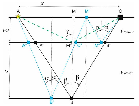
Figure 1.
Ray paths from a source (point A) to a receiver (point C): primary reflections from the seafloor (dashed green line) and the layer bottom (continuous black line), and a peg-leg multiple reflection (dashed blue line).
In a field experiment, the measured values are the Tabc and Tpl travel times from the primary ABC and peg-leg multiple. In the following text, we use bold fonts for known values, to distinguish them from the unknowns during the computation flow; the unknowns are in plain, italic font. We assume that the seawater velocity Vw is also known, as a standard value of 1500 m/s is very often found. However, seasonal temperatures may affect this velocity by varying it in a range from 1440 to 1540 m/s (see, e.g., [13]). If temperature and salinity are known, the formula of Mackenzie [14] can be used for it. The water depth Wd may be known from bathymetric maps or measured either directly by sonar or indirectly by inverting the Twd travel time of the primary reflection from the seafloor. The offset X is measured along the cable length that is trailing the source and receiver. If significant deviations are expected, due to feathering effects [15,16], an alternative measurement for X is provided by the Td travel time of the direct arrival, multiplied by the seawater velocity Vw. Thus, in any of these different ways, we may assume that X, Wd, and Vw, as well as Tabc and Tpl, are known. With this information, the layer thickness Lt and its velocity Vlayer can be estimated.
2.1. Peg-Leg Multiples
The Tabc and Tpl travel times provide the following two equations:
where two additional unknowns α and β appear (Figure 1). They are the incidence angles for the peg-leg multiple and for the primary reflection from the lower layer bottom. We need two more equations to obtain a viable solution, which can be obtained by trigonometric relations as follows:
Tabc = Taa′ + Ta′b + Tbb′ + Tb′c = 2 (Taa′ + Ta′b) = 2 (Wd/Vw + Lt/Vlayer)/cosβ
Tpl = 2 (Taa″ + Ta″b″ + Tm′m″) = 2 (2 Wd/Vw + Lt/Vlayer)/cosα
tanβ = AM/(MM* + M*B) = X/[2 (Wd + Lt)]
X = 2 [(MM* + M*B) + MM*] tanα = 2 (2 Wd + Lt) tanα
Equations (2)–(5) form a nonlinear system in the four unknowns α, β, Lt, Vlayer that can be solved numerically with a few constraints as follows:
where γ is the incidence angle of the primary reflection from the seafloor. To reduce the computational efforts, we can simplify this equation system by defining the ratio LV as
0 < α < β < γ = atan(0.5 X/Wd), X > 0, Lt > 0
LV = Lt/Vlayer
Substituting (7) in (2) and (3) and rearranging, we obtain
Tabc cosβ = 2 (Wd/Vw + LV) = 2 Wd/Vw + 2 LV
Tpl cosα = 2 (2 Wd/Vw + LV) = 4 Wd/Vw + 2 LV
tanβ =X/[2 (Wd + Lt)]
tanα = X/[2 (2 Wd + Lt)]
By subtracting (8) from (9), we obtain a system of three equations with three unknowns (α, β, and Lt) as follows:
Tpl cosα − Tabc cosβ = 2 Wd/Vw
tanβ =X/[2 (Wd + Lt)]
tanα = X/[2 (2 Wd + Lt)]
Rearranging (13) and (14), we obtain
2 Wd + 2 Lt = X/tanβ
4 Wd + 2 Lt = X/tanα
Subtracting (12) from (13), together with (12), we obtain a system of two nonlinear equations with two unknowns (α and β) as follows:
which can be solved numerically with the constraints (5). When α and β are computed, we can obtain the layer thickness Lt using Equation (13) or (14). For example, from (14),
where we use the bold font for tanα to highlight that the α angle becomes a known value at this point. The LV product, similarly, can be obtained by either (8) or (9). Using (8), for example, we have
Tpl cosα − Tabc cosβ = 2 Wd/Vw
X/tanα − X/tanβ = 2 Wd
Lt = 0.5 X/tanα − 2 Wd
LV = 0.5 Tabc cosβ − Wd/Vw
Substituting LV in (7), we obtain the last unknown Vlayer as follows:
Vlayer = Lt/LV
2.2. Intrabed Multiples
Another common type of multiple reflection in marine surveys is an internal bounce in the shallowest layer below the seafloor, often composed of unconsolidated sediments overlying stiffer rocks. Figure 2 shows this intrabed multiple with the ray path AA″B″M′C″M″C (blue dotted line). It is convenient to draw also the mirrored point B* of the bouncing point M′, with respect to the reflection point B. In other words, we add a mirrored layer (in red) below the investigated layer.
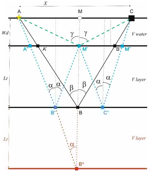
Figure 2.
Ray paths from a source (point A) to a receiver (point C): primary reflections from the seafloor (dashed green line) and the layer bottom (continuous black line), and an intrabed multiple reflection (dashed blue line). The red lines indicate a virtual specular layer below the actual one and a virtual ray path.
To estimate Lt and Vlayer in this case, we proceed in a similar way as for the peg-leg multiples. The Tabc travel time provides the same equation as Equation (2), and the incidence angle β provides the same Equation (4). The Tib travel time for the intrabed multiple is slightly different, defines as follows:
Tib = 2 (Taa″ + Ta″b″ + Tb″m′) = 2 (Wd/Vw + 2 Lt/Vlayer)/cosα
Additionally, the fourth equation needed to complete the system is also slightly different, which is expressed as follows:
tanα = AM/(MM′ + M′B + BB*) = AM/(MM′ + 2 M′B) = X/[2 (Wd + 2 Lt)]
By the same process of substituting Equation (7) and rearranging, we obtain another set of nonlinear equations as follows:
Tabc cosβ = 2 (Wd/Vw + LV)
Tib cosα = 2 (Wd/Vw + 2 LV)
tanβ = X/[2 (Wd + Lt)]
tanα = X/[2 (Wd + 2 Lt)]
Rearranging (24), we attain for 2 LV
Tabc cosβ − 2 Wd/Vw = 2 LV
Substituting (28) in (25), and manipulating (26) and (27), we obtain
Tib cosα = 2 (Tabc cosβ − Wd/Vw)
Lt = 0.5 X/tanβ − Wd
2 Lt = 0.5 X/tanα − Wd
Substituting (30) in (31) and rearranging, we achieve a system of two equations with two unknowns (α and β) as follows:
which can be solved numerically as in the previous case, with the same constraints (6). The layer thickness Lt can be obtained from (30), the ratio LV from (28), and the velocity Vlayer from (21).
Tib cosα − 2 Tabc cosβ = −2 Wd/Vw
0.5 X/tanα − X/tanβ = −Wd
LV = 0.5 Tabc cosβ − Wd/Vw
3. Synthetic Data Example
To validate the algorithm presented above, we built a simple 1.5-D model composed of horizontal interfaces. The upper layer represents the seawater, with a constant velocity of 1500 m/s and a thickness of 20 m. In the layer below the seafloor, the velocity varied smoothly, with a Gaussian curve between 2000 and 2500 m/s (Figure 3a). Below the layer, a half-space with a velocity of 2600 m/s was placed for plotting purposes only. We simulated the travel times for 50 traces, calculating the direct arrivals, the primary reflections from the seafloor and the layer bottom, and the intrabed multiple inside that second layer. The offset was set to 2.5 m only, although values up to 10 m may be encountered in practice. We neglected the ray bending, which is fine for the water bottom primary and the direct arrival, as it is a fair approximation for the other events only when the offset between source and receiver is small with respect to the depth of the sea and the deeper interfaces. When plotting the model in the time domain (Figure 3b), the travel times of the primary reflections below the velocity anomaly showed a typical pull-up effect, distorting the actual flatness of the layer bottom. Thus, correct imaging requires quantifying and compensating that velocity anomaly.
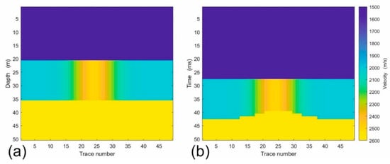
Figure 3.
Synthetic model with horizontal interfaces and a Gaussian velocity anomaly in the depth domain (a) and in the time domain (b).
The inversion of the simulated travel times for direct arrivals, primaries, and multiples provided estimates that are astonishingly precise, with errors lower than 0.2% [17], but this encouraging result was obtained without errors or noise affecting our input data. Additionally, the forward and inverse modeling were based on the same ray tracing algorithm, so no further drawbacks appeared due to the propagation effects, such as anelastic absorption, source, and receiver radiation pattern, and incidence-angle-dependent phase rotations. For these reasons, we tested the estimation robustness with respect to data errors.
The circles in Figure 4a show the estimated velocity–thickness couples in the layer below the seafloor, when perturbing the offset of each trace 40 times by random errors up to 1% while keeping the travel times of the reflections correct as modeled. Dots with the same color correspond to the same trace simulated in the model in Figure 3, i.e., in the same location for source and receiver: On the left, the traces are plotted at the model sides, where the velocity is 2000 m/s, whereas moving to the right, the traces are observed in the central part of the model, where the velocity anomaly tops to 2500 m/s. We clearly notice a linear trend for each group of perturbations for the same trace. By averaging the couples for each trace perturbation (thick blue line), the correct value of 15 m is fairly approximated for the layer thickness, while the velocity spans its actual interval.
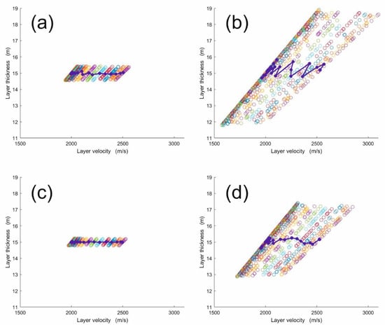
Figure 4.
The circles present the estimated layer velocity and thickness obtained by perturbing randomly the input data in different ways. Dots with the same color correspond to the same perturbed offset along the profile over the model in Figure 3. The correct thickness is 15 m, while the velocity ranges from 2000 to 2500 m/s. The thick blue line joins the averages of the perturbed offsets in each line. The perturbations are (a) the offset, up to 1%; (b) the intrabed multiple, up to 0.01% with a 2.5 m offset, (c) with a 10 m offset, and (d) with 0.1% perturbation but still with a 10 m offset.
Figure 4a shows that a 1% error in the offset (i.e., 2.5 cm in this example) may produce errors up to 0.4 m (2.6%) in the layer thickness and 70 m/s (2.8%) in the layer velocity; thus, high precision is needed in the offset measurement. Effects of cable feathering and sea waves [18] must be compensated for at each trace; in addition, averaging the estimates in adjacent traces may also reduce the instabilities. The numerical solver we adopted for the equation system (24–27) was an exhaustive search in a grid 3000 × 3000, subject to the constraints in Equation (6). More accurate (but more complex) algorithms exist, which may improve the estimation accuracy further.
In actual data processing, the most challenging task is to select the multiple reflections properly. Recognizing them is just the first step. For the peg-leg multiples, we can compare the travel time from the seafloor with the time differences between other major events. Intrabed multiples are far more elusive, but crossing events may offer hints to distinguish them. However, crossing events have also a drawback—they distort the waveform and may delay or anticipate their main peaks. Another problem is the anelastic absorption, which reduces the high-frequency content in the multiples with respect to the corresponding primary, again introducing a delay in its waveform peak. Finally, assigning a precise travel time to a minimum-phase signal, as in a Boomer survey, is particularly difficult, as the waveform onset is mostly hidden by the noise or other interfering signals. For these reasons, we also tested the effect of selecting errors in the intrabed multiples and found that this is the most critical value for a reliable inversion of the layer velocity.
When testing random errors in travel times up to 1%, as performed for the offsets, the results were totally disappointing. Only by reducing the perturbation percentage to 0.1%, we obtained the results in Figure 4b. The estimated thickness was slightly bumpy, but the error of the average values (blue dots) still did not exceed 1 m with respect to the actual one of 15 m. Instead, the velocity errors exceeded even 700 m/s, i.e., about 22%, the maximum value of 2500 m/s. As the travel times of the intrabed multiples were about 56 ms, the error should not exceed 56 microseconds, which was close to the sampling interval for Boomer surveys. This extreme precision is hardly achievable in a real experiment unless the data processing before selection can reduce the noise significantly and compensate for the waveforms’ distortion due to the anelastic absorption.
Figure 4c,d show how the uncertainty can be reduced to achieve a better estimate for the layer velocity. The offset was then increased in both cases to 10 m, which is still manageable by a small ship in busy ports. When the perturbation was very small, i.e., 0.01% as for Figure 4b, the maximum velocity error was about 60 m/s, i.e., quite small. When we consider more realistic travel-time errors, such as 0.1% (about 560 microseconds, or 10 sample intervals), the maximum velocity error in the central anomaly was found to be 400 m/s, which is only 16%.
We plotted all parts in Figure 4 using the same scale to highlight the different sensitivity of the two parameters being estimated (layer velocity and thickness) with respect to measurements that are more challenging when dealing with experimental data, i.e., offset and multiple’s travel time. Minor errors in the offset (Figure 4a) caused acceptable errors in both estimates, even when using a short offset of 2.5 m. Instead, travel-time errors were much less forgiving (Figure 4b–d): They required increasing the offset to at least 10 m to achieve a result that is not ideal but still useful in practice (Figure 4d). These figures show also that, for small perturbations, the averages of estimated thickness and velocity at each location (blue lines) may be more or less bumpy but relatively close to the correct values. Thus, multiple folds of the same point in the survey can contribute significantly to the result reliability.
4. Experimental Data Example
As regards processing real marine data with the algorithm described above, a key step is to select the travel times of seismic signals. Apart from the problem of interpreting the multiples as peg-leg or intrabed, which may be interfering with other primaries, the minimum-phase property of the Boomer (or air gun) signal also poses challenges. The travel time for such a signal is the time break of the waveform, that is, the time when the signal amplitude has a burst with respect to the background noise. Its Recognition is easy for direct arrivals and primary reflections from the seafloor but is very difficult for multiples. Normally, to bypass this problem, the maximum (or minimum) peak is selected, and then a time delay is subtracted. This delay can be estimated for a typical waveform directly from the data, e.g., in some primary reflection from the seafloor where the noise contribution is minimum.
Figure 5 shows two minimum-phase wavelets with different frequency bandwidth: The first is 300–9000 Hz, similar to the nominal range of the Boomer source we used; the second is 300–4500 Hz, which can mimic a signal after some propagation in a dissipative medium, as mainly high-frequencies are absorbed. We obtained them by filtering a unit spike at the time zero with minimum-phase Butterworth filters with the frequency ranges mentioned above. The sampling rate was 1 microsecond. If we choose the largest peak of this signal, as we should in practice to overcome the background noise, we obtain two different delays Δ1 and Δ2, where the second is almost double the first one. Therefore, we may have to introduce a time shift in our picked travel times, which is ideally time-dependent. In practice, however, a negative time shift of the order of 0.5 ms may be needed for the arrivals of intrabed or peg-leg multiples.
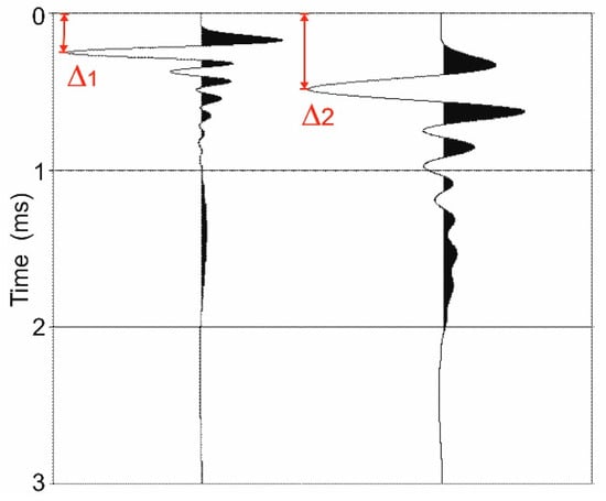
Figure 5.
Two minimum-phase Butterworth wavelets with different bandwidths: 300–9000 Hz (left) and 300–4500 Hz (right). The time delay Δ1 of the main peak from the time origin is about half of the delay Δ2 of the second trace.
Figure 6 shows a Boomer profile acquired in the Gulf of Trieste (Northern Adriatic Sea). The recording system was a Boomer AAE301, with a sampling interval of 10 microseconds and a shooting interval of about 0.7 m. The frequency band ranged from 500 to 6000 Hz. As feathering and sea waves may change the nominal offset between source and receiver, we computed the actual offset at each shot by choosing the direct arrival (red line) and multiplying its travel time by the seawater velocity. This velocity was measured independently, and it was relatively high, i.e., 1532 m/s [19], due to the high salinity and temperature in the area during the survey (see also [20]). The average offset was 4.84 m, with a standard deviation of 5 cm, which is 1%. This relative error was small enough for a fair estimation and comparable to the perturbations in the synthetic example (Figure 4).
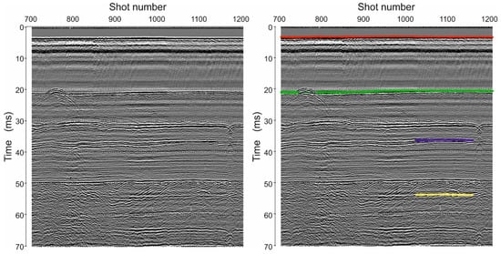
Figure 6.
Seismic section acquired at the Gulf of Trieste (Northern Adriatic Sea) using a Boomer system without (left) and with the selected horizons (right): direct arrival (red), seafloor reflection (green), primary reflection (violet), and peg-leg multiple (yellow).
The other selected horizons shown in Figure 6 are the seafloor (green) reflection and a prominent primary reflection at about 37 ms (dark blue). We preferred this particular event to others because its peg-leg multiple (yellow) was very clear; indeed, it cut dipping interfaces in the central part, at about 55 ms, thus unambiguously revealing its nature of multiple. For the other possible candidate, the reflector at about 32 ms, choosing its peg-leg multiple was relatively fuzzy.
From a geological point of view, the formations between the seafloor and the selected primary are composed of unconsolidated sediments, which may be partially saturated with gas. Above this area, indeed, terrigenous sediments (the Eocene flysch) are present, characterized by seismic diffractions and deformations [21]. The erosion surface at 50 ms is the top of flysch formation. Most of the visible flat events below this surface are multiple reflections.
Figure 7a shows the estimated water depth (orange line), which is very smooth as expected by the visual inspection of the seismic section. Less obvious is the smoothness of the estimated offset (grey line), because surface waves and possible rapid turns in busy areas might introduce irregularities. Slightly less stable is the estimated layer thickness (blue line). Its calculation (and that one of the layer velocity) depend heavily on the selection precision of the multiple and the reflection from the layer bottom. Both travel times may be affected by larger errors because their time break is far less evident than that for direct arrivals and water bottom reflections. For this reason, we applied a five-term median filter to the velocity estimate (Figure 7b). The obtained values ranged between 1500 and 1600 m/s and are well consistent with those measured by [22], a dozen kilometers apart from our study area. These values are average velocities between the layer bottom and the seafloor. We observed that the estimated velocity oscillated above and below the seawater velocity. The low values are likely due to some extent of gas saturation, which is known to occur in several parts of the Gulf of Trieste (see also [23,24], etc.).
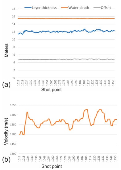
Figure 7.
Estimation results: (a) layer thickness (blue line), water depth (orange line), and offset (grey line); (b) layer velocity after a 5-term median filter.
5. Discussion
Figure 4 exhibits a linear trend of the estimates when perturbating either the offset or the multiples’ travel time at a given location, highlighted by the same color of the corresponding circles. This occurred because of the small incidence angles α and β (Figure 1 and Figure 2) when the offset was short with respect to the layer-bottom depth. In our synthetic example, for a 2.5 m offset,
is almost equal to tanβ = 0.035714. The angle α is even smaller than β, as per Equation (6). Both equation systems (8–11) and (24–27) become more linear if we approximate
using a first-order Taylor series expansion. Only the cosine terms in (8)–(9) and (24)–(25) maintain a mild nonlinearity in the equations. Thus, if perturbing one of the four variables at a time, as in our examples, we may expect (quasi)linear variations in the solutions, i.e., in terms of the layer thickness and its velocity.
β = atan(0.5 X/(Wd + Lt)) = atan(0.5 × 2.5/(20 + 15)) = 0.035699
tanα ≈ α, tanβ ≈ β
The perturbation results in Figure 4 were obtained for a short offset of 2.5 m to match our field experiment and, in general, a convenient option for operations in busy or environmentally fragile areas. In the framework of crustal studies, Majdanski [25] studied analytically the relation between offset and the uncertainties in the layer velocity and thickness. Perturbing the travel times similarly to our study, he showed that, for short offsets, variance in the estimated thickness is larger than that of velocities, while the opposite occurs in large offsets. Thus, in our case, we may rely on estimates of thickness more than velocity. When the latter parameter is more critical for offshore engineers, extending the cable may help. Of course, when reliability and resolution must be maximized, a multichannel survey and a reflection-refraction tomography provide high-quality images in depth [9], even for time-lapse surveys in complex geological structures [13,26]. The joint inversion of direct, reflected, and refracted arrivals increases the areal coverage and local density of rays, stabilizing the tomographic inversion and increasing its robustness with respect to the noise. Therefore, when just a single channel is available, the joint inversion of different multiples is a way forward for possible improvements.
Recognizing multiples is easy only for the “simple” ones, i.e., those whose travel time is (about) twice that of the corresponding primaries. In that case, the related signal amplitude is also relatively prominent. Peg-leg and intrabed multiples are weaker and more challenging, requiring ideally a preliminary tentative selection and a careful comparison of travel times: to the travel time of a deep primary, we must add the travel time of the seafloor or the estimated transit time across some layer interval. Often, this can be performed safely only in limited parts of a survey.
The presented equations and method assume horizontal interfaces layers and homogeneous layers. When minor deviations from these hypotheses occur, the result is acceptable. Otherwise, a full tomographic approach and multichannel surveys are needed.
6. Conclusions
We presented an algorithm for estimating the velocity and thickness of a layer below the seafloor by a monochannel acquisition system, by inverting the travel time of direct arrivals, as well as primary and multiple reflections. A nonlinear set of equations was obtained that can be solved numerically with high precision. However, when measurement errors occur in the input data, due to travel-time selection errors or just ambient noise in the survey, severe instabilities emerged. We showed that a very short offset (2.5 m) can estimate only the layer thickness fairly, while at least a 10 m offset is needed to predict the layer velocity within an acceptable error range.
Real data processing provides additional challenges. A high-frequency source such as a Boomer emits a signal that is rapidly absorbed by the shallow marine sediments. This absorption modifies the signal waveform during its propagation so that direct arrivals, primaries, and multiples have different delays between their first onset and their peak. We showed that a shift may be needed to improve inversion accuracy if the time break of a waveform can be hardly distinguished from the background noise.
Our method for estimating velocity and thickness in a layer below the seafloor using a peg-leg multiple was validated by a real dataset, i.e., a short-offset Boomer survey acquired at the Gulf of Trieste (Northern Adriatic Sea). The obtained values were in good agreement with studies in a nearby area, where borehole ties are also available.
Author Contributions
L.B. contributed with the key ideas, the data acquisition, and its processing; A.V. developed the mathematical algorithm, its software implementation, and the basic text. Both authors contributed to the discussion, the conclusions, and the final text revision. All authors have read and agreed to the published version of the manuscript.
Funding
This research received no external funding.
Institutional Review Board Statement
Not Applicable.
Informed Consent Statement
Not Applicable.
Data Availability Statement
The experimental data presented in this paper was acquired under confidentiality conditions. The synthetic example data and the developed MATLAB code can be provided by the corresponding author (avesnaver@ogs.it) upon request.
Acknowledgments
We thank our colleagues at OGS that contributed to the Boomer data acquisition.
Conflicts of Interest
The authors declare no conflict of interest.
References
- Trabant, P.K. Applied High-Resolution Geophysical Methods; Springer: Dordrecht, The Netherlands, 1984; 265p, ISBN 978-94-009-6495-2. [Google Scholar]
- Lee, H.-Y.; Park, K.-P.; Koo, N.-H.; Yoo, D.-G.; Kang, D.-H.; Kim, Y.-G.; Hwang, K.-D.; Kim, J.-C. High-resolution shallow marine seismic surveys off Busan and Pohang, Korea, using a small-scale multichannel system. J. Appl. Geophys. 2004, 56, 1–15. [Google Scholar] [CrossRef]
- Baradello, L.; Carcione, J.M. Optimal seismic-data acquisition in very shallow waters: Surveys in the Venice lagoon. Geophysics 2008, 73, Q59–Q63. [Google Scholar] [CrossRef]
- Richardson, W.J.; Greene, C.R.; Malme, C.I.; Thomson, D.H. Marine Mammals and Noise; Academic Press: San Diego, CA, USA, 1998; ISBN 9780080573038. [Google Scholar]
- Gordon, J.; Gillespie, D.; Potter, J.; Frantzis, A.; Simmonds, M.P.; Swift, R.; Thompson, D. A review of the effects of seismic surveys on marine mammals. Mar. Technol. Soc. J. 2003, 37, 16–34. [Google Scholar] [CrossRef] [Green Version]
- Verbeek, N.H.; McGee, T.M. Characteristics of high-resolution marine reflection profile sources. J. Appl. Geophys. 1995, 33, 251–269. [Google Scholar] [CrossRef]
- Kosloff, D.; Sherwood, J.; Koren, Z.; Machet, E.; Falkovitz, Y. Velocity and interface depth determination by tomography of depth migrated gathers. Geophysics 1996, 61, 1245–1569. [Google Scholar] [CrossRef] [Green Version]
- Mosher, D.C.; Simpkin, P.G. Status and trends of marine high-resolution seismic reflection profiling: Data acquisition. Geosci. Can. 1999, 26, 174–188. [Google Scholar]
- Nolet, G. A Breviary of Seismic Tomography; Cambridge University Press: Cambridge, UK, 2011; 344p, ISBN 9780511984709. [Google Scholar] [CrossRef]
- Denich, E.; Vesnaver, A.; Baradello, L. Amplitude recovery and deconvolution of Chirp and Boomer data for marine geology and offshore engineering. Energies 2021, 14, 5704. [Google Scholar] [CrossRef]
- Green, C.H. Velocity determination by means of reflection profiles. Geophysics 1938, 3, 295–305. [Google Scholar] [CrossRef]
- Alkhalifah, T.A. Full Waveform Inversion in an Anisotropic World; Education Tour Series; EAGE: Houten, The Netherlands, 2014; 197p, ISBN 9789462822023. [Google Scholar]
- Vesnaver, A.; Accaino, F.; Böhm, G.; Madrussani, G.; Pajchel, J.; Rossi, G.; Dal Moro, G. Time-lapse tomography. Geophysics 2003, 68, 815–823. [Google Scholar] [CrossRef]
- Mackenzie, K.V. Nine-term equation for sound speed in the oceans. J. Acoust. Soc. Am. 1981, 70, 807–812. [Google Scholar] [CrossRef]
- Levin, F.K. The effect of streamer feathering on stacking. Geophysics 1983, 48, 1165–1171. [Google Scholar] [CrossRef]
- Sirgue, L.; Xia, G. Impact of feathering on imaging for wide azimuth data. SEG Annu. Meet. 2008, 1003–1007. [Google Scholar] [CrossRef]
- Vesnaver, A.; Baradello, L. Shallow velocity estimation by multiples in Boomer surveys. Annu. Meet. 2022. submitted. [Google Scholar] [CrossRef]
- Tosi, L.; Rizzetto, F.; Zecchin, M.; Brancolini, G.; Baradello, L. Morphostratigraphic framework of the Venice Lagoon (Italy) by very shallow water VHRS surveys: Evidence of radical changes triggered by human-induced river diversions. Geophys. Res. Lett. 2009, 36, 1–5. [Google Scholar] [CrossRef]
- Affatato, A.; Baradello, L.; Cotterle, D.; Deponte, M.; Petronio, L.; Sorgo, D. Rilievo Geofisico MOLO VIII (Trieste); Report, Sezione GEO 22; OGS: Trieste, Italy, 2021. [Google Scholar]
- Diviacco, P.; Nadali, A.; Iurcev, M.; Carbajales, R.; Busato, A.; Pavan, A.; Burca, M.; Grio, L.; Nolich, M.; Molinaro, A.; et al. MaDCrow, a citizen science infrastructure to monitor water quality in the Gulf of Trieste (North Adriatic Sea). Front. Mar. Sci. 2021, 8, 619898. [Google Scholar] [CrossRef]
- Busetti, M.; Volpi, V.; Nicolich, R.; Barison, E.; Romeo, R.; Baradello, L.; Brancatelli, G.; Giustiniani, M.; Marchi, M.; Zanolla, C.; et al. Dinaric tectonic features in the Gulf of Trieste (Northern Adriatic Sea). Bull. Geophys. Oceanogr. 2010, 51, 117–128. [Google Scholar]
- Novak, A.; Smuc, A.; Poglaien, S.; Celarc, B.; Vrabec, M. Sound velocity in a thin shallowly submerged terrestrial-marine Quaternary succession (Northern Adriatic Sea). Water 2020, 12, 560. [Google Scholar] [CrossRef] [Green Version]
- Carcione, J.M.; Poletto, F. Sound velocity of drilling mud saturated with reservoir gas. Geophysics 2000, 65, 646–651. [Google Scholar] [CrossRef]
- Vesnaver, A.; Busetti, M.; Baradello, L. Chirp data processing for fluid flow detection at the Gulf of Trieste (Northern Adriatic Sea). Bull. Geophys. Oceanogr. 2021, 62, 365–386. [Google Scholar] [CrossRef]
- Majdański, M. The uncertainty in layered models from wide-angle seismic data. Geophysics 2013, 78, WB31–WB36. [Google Scholar] [CrossRef]
- Vesnaver, A.; Lin, R. Broadband Q-factor tomography for reservoir monitoring. J. Appl. Geophys. 2019, 165, 1–15. [Google Scholar] [CrossRef]
Publisher’s Note: MDPI stays neutral with regard to jurisdictional claims in published maps and institutional affiliations. |
© 2022 by the authors. Licensee MDPI, Basel, Switzerland. This article is an open access article distributed under the terms and conditions of the Creative Commons Attribution (CC BY) license (https://creativecommons.org/licenses/by/4.0/).