Location Optimisation in the Process of Designing Infrastructure of Point Pollutant Emitters to Meet Specific Environmental Protection Standards

Abstract

This article addresses the challenge of searching for the optimal location for a newly designed pollutant emitter (new factory or other facility) in relation to the requirements imposed by environmental protection regulations on the concentrations of selected pollutants in a given area, taking into account the currently existing levels of analysed substances. The paper presents the key issues of the dispersion of pollutants in atmospheric air and pollutant dispersion models. The Gaussian model of a plume, based on the Pasquill diffusion equation, is chosen to simulate the dispersion of pollutants in atmospheric air. The key issue within the paper constitutes the research section responsible for using the Monte Carlo global optimisation method in order to find the optimal location. The proposed algorithm is intended to offer measurable and subjective arguments and options to preliminary discussions on choosing a location for new factories, while such discussions choices should be fact-based and ecologically acceptable instead of fulfilling only political or economical goals. The paper is intended to present the need for easily interpretable arguments for discussions and responsible decisions on choosing the lowest-impact location of pollutant emitters to the scientific community.

1. Introduction

Finding the right location for a new industry site is a challenging problem. Every time, vivid discussion among decision-makers takes various aspects into consideration. This paper is intended to help the scientific staff of those companies/institutions in articulating the need for leveraging the environment-oriented arguments rather than political or economical ones. The paper offers easily interpretable, law-compliant methods, equipped with optimisation for choosing the lowest-impact location.

Brief Introduction to Pollutant Dispersion

The gaseous envelope surrounding the Earth, as well as other planets in the Solar System, is called the atmosphere. The gases contained in the Earth’s atmosphere create atmospheric air. Its permanent components are [1]:

• molecular nitrogen $N_2$ in excess of $78\%$;
• oxygen $O_2$, slightly less than $21\%$;
• argon $Ar$, $0,9\%$;
• neon $Ne$, helium $He$, krypton $Kr$, xenon $Xe$;
• hydrogen $H_2$, ozone $O_3$ in trace quantities.

The emission of atmospheric air pollution takes place in the lowest layer of the atmosphere—the troposphere [1]. This dependence is crucial because the mechanisms that allow the dispersion are taking place in this particular layer.

The composition of the atmosphere is strictly defined, and any exceeding of the set standard becomes pollution. The pollutants that are emitted into the atmosphere have a destructive impact on human health as well as on the environment [2,3]. However, this occurs not only in the immediate vicinity of emission sources, as the observed effects are global in nature [4]. Any emission is always connected with the process of propagation caused by the circulation of air masses, which is influenced by many factors correlated with the characteristics of the land [5] as well as with meteorological conditions [6,7]. In view of the harmful effects on human health, the most dangerous group are dust particles (named Particulate Matter, PM, in the literature), which, due to their particle size, penetrate deep into the lungs and then are able, like oxygen, to enter the circulatory system. Depending on the particle size, differentiation is made between [8]:

• PM 10—particulate matter fractions of aerodynamic diameter in the range: (2.5 $\mathsf{\mu }$m; 10 $\mathsf{\mu }$m);
• PM 2.5—particulate matter fractions up to 2.5 $\mathsf{\mu }$m in diameter;
• TSP—total suspended particulate matter.

Places from which harmful substances are released into the atmosphere are referred to as sources of pollution:

• Natural sources, related to the functioning of nature;
• Man-made sources, related to human activity.

Man-made sources of pollutant emission can be divided into [9,10]:

• Point sources—the release of pollutants into the atmosphere takes place in a volume much smaller than the considered pollutant transport distance (chimneys [11], ventilation shafts, households);
• Linear sources—the release of pollutants into the atmosphere takes place along a straight line or curve of a length comparable to the considered pollutant transport distance (roads [12], motorways, open sewage channels). For the purposes of calculation, such an emission may be treated as a set of point sources;
• Surface sources—the release of pollutants into the atmosphere takes place from a plane, and the dimensions of the plane are comparable to the considered pollutant transport distance (re-emission of pollutants from waters [13], sedimentation tanks, waste dumps);
• Volumetric sources—the release of pollutants into the atmosphere takes place in a volume of dimensions comparable to the considered transport distance (e.g., volcanic emission [14] including emission from lava and ash clouds).

The process of dispersion of pollutants in atmospheric air is characterised by a description containing complex parameters, which are variable both in time and space [15]. To deal with this class of issues, a number of mathematical and physical models have been developed and are now being applied for decisions related to improving air quality in the light of the developing infrastructure [16].

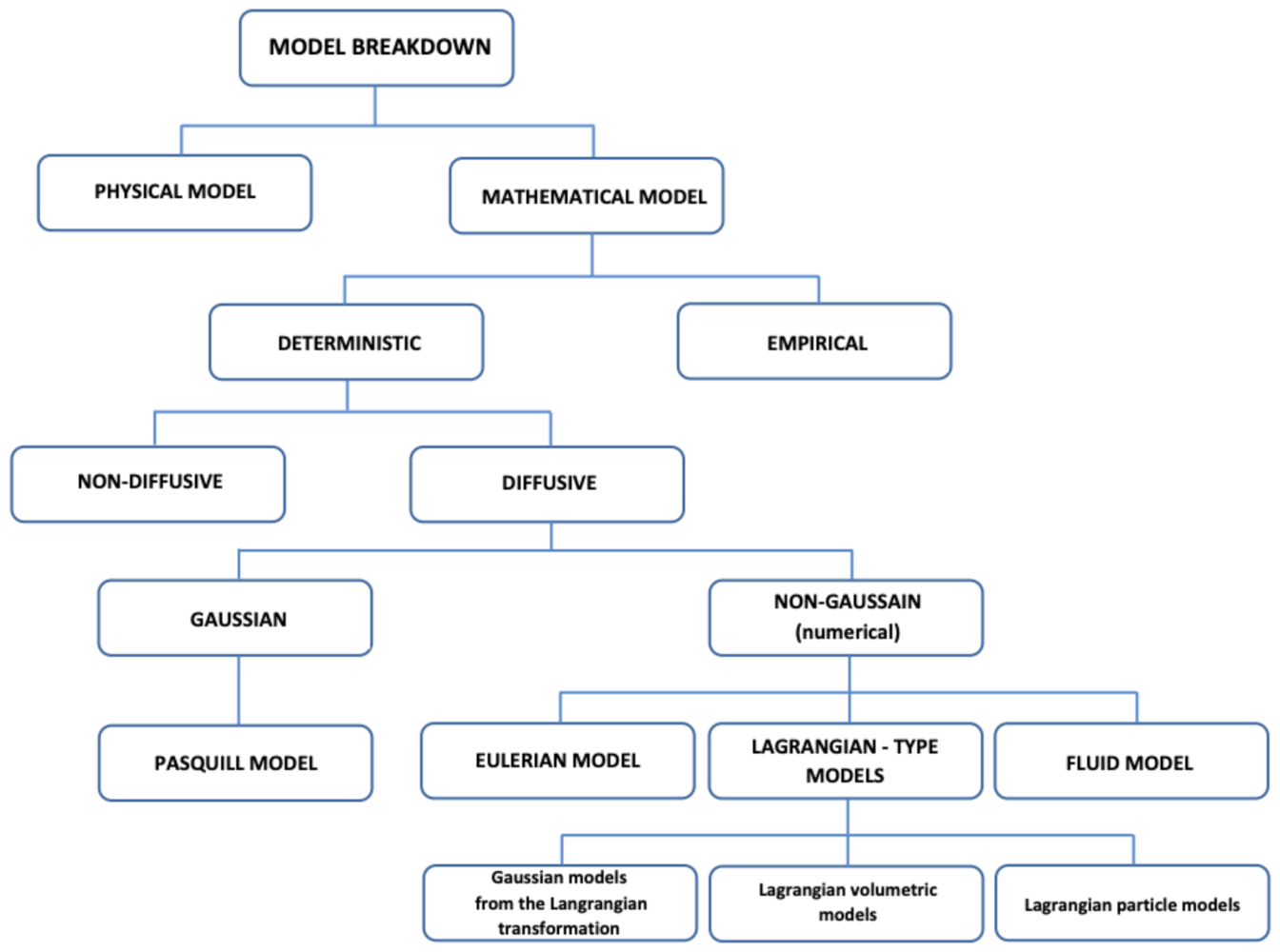
2. Pollutant Dispersion Models

The process of modelling the dispersion of pollutants in the atmosphere is currently a key issue raised at many levels of research [17,18,19]. This is due to the ever-increasing possibilities to implement models of atmospheric dispersion [5]. They are used increasingly to predict future concentrations of substances likely to have a negative impact on the health of living organisms [2,20] as well as the resulting environmental effects [16]. The number of companies and institutions involved in the development of forecasting models focused on the impact of pollution on the local environment [21] related to the development of industrial infrastructure is constantly increasing [18,19].

For the purpose of these activities, models of atmospheric air pollution dispersion are used [22,23], which are categorised into two main groups:

• Physical models—developed in laboratory conditions, where the whole process is carried out on the basis of simulation, just like in the real atmosphere. They are the basis for creating mathematical models;
• Mathematical models—describe chemical processes that take place in the atmosphere using numerical methods—analytically. These are often referred to as deterministic models in which description of phenomena taking place in the atmosphere is conducted using mathematical equations.

It is also possible to draw up a description of these correlations using the relationships presented in (Figure 1).

According to the state administration regulations in Poland, the Pasquill formula [25], which is a Gaussian model, is used to determine the state of air pollution associated with existing or planned emission sources [26]. The Pasquill study contains a simplified gas pollution diffusion equation located in a moving gas medium [25,27].

2.1. Gaussian-Type Models—Old Generation Plumes

The old-generation Gaussian plume models use the traditional description of the intensity of turbulent movements in the atmosphere. There are discreet states of atmosphere equilibrium. The key issues of such models are oriented around:

• The description of turbulent diffusion, i.e., determination of standard deviations of the distribution of pollutant concentrations in the plume (${\sigma }_y$ and ${\sigma }_z$);
• Determining the effective height of the emitter $H_p$;
• Determining the average wind speed in the layer of dispersion of pollutants $U_{sr}$.

These models are usually used to assess the air pollution on a local scale. Their advantage is the simplicity of handling, as well as the ease of access to data necessary to perform calculations. The low complexity of the calculations makes them widely used, despite the numerous limitations of the simplifications adopted.

2.2. New Generation Models with the Gaussian Module

New generation plume models eliminate the traditional description of turbulence structure in the atmosphere—discrete states of equilibrium are replaced by elements based on the use of probability theory related to the parameters of the boundary layer of the atmosphere. This allows a new parameterisation for the turbulent diffusion process. The convective parameters of the boundary layer are used, which include:

• Surface heat flux $H_0$;
• Surface momentum flux ${\tau }_0$;
• Thickness of the atmosphere boundary layer $h_{bl}$.

The parameters listed above are used to determine the following values:

• Frictional speed $u_{\ast }$;
• Monin—Obukhov length scale L;
• Potential temperature scale ${\theta }_{\ast }$;
• Convective speed scale $w_{\ast }$.

Working with this model usually requires access to a more detailed level of information than publicly available. (The data referred to in this paragraph include a set of meteorographic information about the analyzed area as well as coefficients related to the description of the surface of this area. Some of the necessary information can be obtained from meteorological websites or stations or basic terrain maps, but other (e.g., terrain details and coefficients) have to be provided by local/regional government centers). The module enabling the processing of meteorological data into parameters characterising the boundary layer determining the vertical wind turbulence and temperature profiles is referred to as a meteorological preprocessor. It therefore prepares the data used for subsequent calculations.

2.3. Gaussian-Type Models of Segmented Plumes

Models of this type are referred to in the literature as models enabling simulation of the process of dispersion of pollutants in the air under inhomogeneous and non-stationary conditions. In addition to typical segmented and puff models, mixed models are also used as their combination. Their use is mainly limited to the process of simulating the dispersion of pollutants on a regional scale. The main limitation of their use is the relatively complicated construction associated with the need to record a large number of puffs moving in the analysed area, which generates considerable calculation costs.

2.4. Gaussian-Type Model—Pasquill Formula

The starting point for most models of dispersion of pollutants in the air is a differential equation describing turbulence diffusion [25] in the following form:

$$\begin{array}{c}\frac{\partial C}{\partial t}+u\frac{\partial C}{\partial x}+v\frac{\partial C}{\partial y}+w\frac{\partial C}{\partial z}=\hfill \\ =\frac{\partial }{\partial x}\left(K_x\frac{\partial C}{\partial x}\right)+\frac{\partial }{\partial y}\left(K_y\frac{\partial C}{\partial y}\right)+\frac{\partial }{\partial z}\left(K_z\frac{\partial C}{\partial z}\right)+S_c\hfill \end{array}$$

(1)

where:

• C—concentration of pollution;
• t—time;
• u, v, w—wind speed vector components;
• x, y, z—coordinates of the location of a point in space;
• $K_x$, $K_y$, $K_z$—components of the atmosphere turbulence diffusion coefficient;
• $S_C$—term describing losses and sources of pollution in the atmosphere.

The solution to Equation (1) can be made using different numerical or analytical methods, but the analytical solution requires a number of simplifications. One of the most frequently used ways of dealing with the discussed problem is to apply the Gaussian formula concerning the propagation of pollution emitted by point-type sources, taking into account the negligence of both spatial and temporal variability of meteorological parameters.

$$C_{x,y,z}=\frac{E}{2\pi U_{sr}{\sigma }_y{\sigma }_z}\times e^{\left(-\frac{y^2}{2{\sigma }_y^2}\right)}\times \left[e^{\left(-\frac{{\left(z-H_e\right)}^2}{2{\sigma }_z^2}\right)}+e^{\left(-\frac{{\left(z+H_e\right)}^2}{2{\sigma }_z^2}\right)}\right]$$

(2)

where: C(x,y,z)—concentration of the pollutant at the point(x, y, z). An extremely important transformation is the introduction of empirical dependence of plume dispersion coefficients determining its distance from the source (2). The obtained relation is described in the literature under the name of Pasquill formula [25,28]. Use in analyses of the dispersion of pollutants in the air in accordance with this principle is optimal if the average wind speed, $U_{sr}$, is greater than $1\frac{m}{s}$. In order to show how the distribution of a plume of pollutants for a point source with continuous emissions fixed over time is analysed, the diagram presented in the following Figure 2 is used.

In Poland, according to the Regulation of the Ministry of the Environment from 5th December 2002, the Gaussian model—the Pasquill formula—is used to determine the state of air pollution for existing or planned sources [26].

3. Optimisation

The optimisation process is a search for a space for possible solutions to the problem in question in order to find the best solution meeting the given criterion [30]. Issues of this kind have dominated in most areas of human life in recent years, and solving them involves the need to know how to obtain appropriate results [31]. The best possible solutions will be formulated as optimal solutions [30]. Optimisation methods are divided into two main classes:

• Deterministic methods [32], which include the golden-section search, the Fibonacci search technique and square interpolation;
• Non-deterministic methods [33], which include genetic algorithms, evolutionary algorithms and the Monte Carlo method [34,35,36,37].

For the purpose of this article, the Monte Carlo (MC) method was used for analysis and calculation.

The MC methods are a set of methods using a random element during operation to solve complex and often complicated problems that cannot be solved using an analytical approach. The MC method relies on numerical calculations, while using random variables to transform the numerical issue of the problem into a probabilistic calculation task, leading ultimately to the same result. The MC method can be used wherever the analyzed problem can be described theoretically in terms of stochasticity, (despite the fact that the analyzed problem can be strictly deterministic). An additional advantage of the MC method is the simplicity of operation and the possibility of parallel implementation. Mathematically, the MC method is based on the task of approximating the expected number $E\left(X\right)$, and the random variable X [34,37].

$$E\left(X\right)=\frac{1}{b-a}\underset{a}{\overset{b}{\int }}f\left(x\right)dx$$

(3)

where:

• $E\left(X\right)$—expected value;
• $f\left(x\right)$—linear function,;
• a, b—interval boundaries.

Taking into account the law of large numbers, it can be assumed that with a relatively large value of n, when the probability is close to 1, the expected value of $E\left(X\right)$ can be approximated to the average $\left(X\right)$:

$$E\left(X\right)\underset{n\to \infty }{\to }\frac{1}{n}\sum _{i=1}^n{x}_i$$

(4)

where:

• n—number of simulations.

Summarising the above dependencies, using a sufficiently high number of simulations, this method allows one to obtain a solution that is average. The use of the MC method is possible wherever a similarity can be found between the target and the presumed behaviour. What distinguishes this optimisation method from the others is the fact that it can be used in any arrangement for which it is possible to formulate the problem in such a way that random elements can lead to a correct result. To sum up, the MC method can be applied in many areas of everyday life [34], mainly in Information Technology, Physics, Economics, Management, as well as in Medicine [38] and other branches of science [35].

4. Identification of the Research Problem

The research problem is identified by creating a computer application that can be used to solve the task of optimal distribution of point pollutant emitters in a specific area [4], while meeting the requirements imposed by environmental regulations. In order to implement the solution to the assumed task, a program was developed to simulate the process of dispersion of pollutants in the air based on the Pasquill plume model, used in Poland in accordance with the recommendations of the Ministry of the Environment when issuing permits for levels of emission of harmful substances into the atmosphere. It has also become necessary to create maps of the area covered by the calculations in such a way as to allow the use of real land cover parameters together with the values of existing pollution. The area of the Opole County together with the city of Opole was used as the example research area. The data took into account the values of the land roughness coefficient and real pollutants, and the calculation grid interval limited to l00 m ensured appropriate precision of the results obtained. The value of the roughness coefficient for the city of Opole, due to the number of inhabitants (in the range of 100,000–150,000), was set at Level 3. The analysis was limited to the concentration of PM 10. It is worth noting that the above method can be used both for gaseous and particulate pollution of other parameters.

5. Implementation of the Methods and Algorithms Used

In order to calculate the values of pollutants in the air, it is necessary to collect a series of input data. The scope and range of meteorological data was limited to a 30-day period, taking into account both day and night measurements. The data were collected for the grid described within the documentation for the voivodeship area, in order to enter data easily into the computational model. Detailed analysis of results for the area is beyond the scope of this paper, therefore the meteorological condition’s variability resulting from different seasons, the time of year, unexpected situations, anomalies or particular weather conditions was not considered.

5.1. Meteorological Data

The necessary meteorological data [16] include:

• The wind speed measured at the anemometer height;
• The average air temperature during the calculation period;
• The atmosphere equilibrium state.

According to the classification of the atmosphere equilibrium state, there are six stability classes. They correspond to the assigned wind speed ranges

Table 1. Wind speed ranges assigned to atmospheric equilibrium states according to the classification of the IMWM [29,39].

Atmosphere Equilibrium State ATM	Wind Speed Component Range [m/s]
Strongly unstable—1 (A)	1–3
Unstable—2 (B)	1–5
Slightly unstable—3 (C)	1–8
Neutral—4 (D)	1–11
Slightly stable—5 (E)	1–5
Stable—6 (F)	1–4

. In case of a stable equilibrium—6 (F) and invariability of other factors influencing dispersion, the pollutant plume remains the longest. In a highly unstable equilibrium—1 (A) the length of the streak is the smallest.

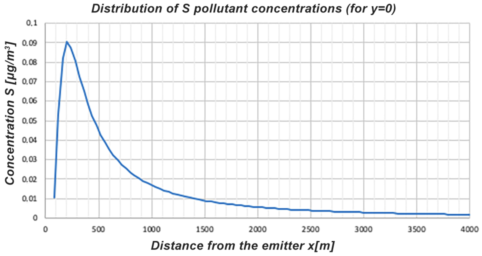
5.2. Receptor Location

The model used requires a description of the exact location of the receptor at the entrance. It involves an introduction of:

• The distance from the emitter (in the axis parallel to the wind direction)—x [m];
• The distance from the emitter (in the axis perpendicular to the wind direction)—y [m];
• The height for which the concentration of the substance is determined—z [m].

5.3. Aerodynamic Roughness Length $Z_0$

Where dispersion takes place in an area with varying topography or height of cover, the degree of intensity of turbulence movements changes. This is due to the varying friction between the surface of the area and the air flowing over it. This relationship is determined by the aerodynamic roughness length $Z_0$ (see

Table 2. Values of the aerodynamic roughness length $Z_0$ [40].

No	Type of Land Cover	Length ${\mathit{Z}}_0$
1.	Water	0.00008
2.	Meadows, pastures	0.02
3.	Cropland	0.035
4.	Orchards, bushes, spinneys	0.4
5.	Forests	2.0
6.	Compact rural development	0.5
7.	City of up to 10 thousand inhabitants	1.0
8.	City of 10 to 100 thousand inhabitants
8.1.	-low buildings	0.5
8.2.	-average buildings	2.0
9.	City of 100 to 500 thousand inhabitants
9.1.	-low buildings	0.5
9.2.	-average buildings	2.0
9.3.	-high buildings	3.0
10.	City of more than 500 thousand inhabitants
10.1.	- low buildings	0.5
10.2.	-average buildings	2.0
10.3.	-high buildings	5.0

).

The aerodynamic roughness coefficient $Z_0$ is a rough generalization, however while it is mentioned and defined in the law [40], using it makes it easier for the results to be accepted by the authorities—it is calculated according to the law. Of course some countries other than Poland may also use other pollutant dispersion models, including Lagrangian particle dispersion models [41], (which seem to give slightly more accurate results [41]), however the authors needed to emphasize the national law-compliant approach.

5.4. Technical Parameters of the Emitter

Each emitter taken into account in the model under consideration should be described with parameters:

• c height of the emitter calculated from ground level—h [m];
• Internal diameter of the emitter outlet—d [m];
• Speed of the substance at the emitter outlet—v [m/s];
• Temperature of the substance at the emitter outlet—T [K];
• Maximum substance emission—E [mg/s].

It is also possible to convert the parameters into emitters with rectangular outlets. The above parameters constitute the set of input data necessary to implement the Pasquill formula. In addition, calculation constants depending on the atmosphere equilibrium factor are also used. The applied algorithm is used to simulate the real process of dispersion of pollutants in the atmosphere. The output data are values of one-hourly concentrations of particulate matter at user-specified distances from the emitter (x, y, z).

For the purpose of applying the optimisation process, it was indispensable to develop maps of the studied area. With the use of QGIS desktop 2.10.18 (multi-platform, user-friendly, free geoinformation program), a model of maps was created according to the assumptions of proper representation of distances in the field. The next step was to move the maps to AutoCAD, where the coordinate grids were superimposed, and individual points with specific $Z_0$-grid values were extracted. As a result of the transformations made, the values of the existing pollution background and $Z_0$ values for individual coordinates were transferred to the text file. The data set, which contained the area of the Opolskie Province, necessary to create the map, was made available on the basis of license number DRP-IV.7522.1.132.2016.JST_16_N by the Marshal of the Opolskie Province.

5.5. Implementation of the Solution, the Posed Optimisation Problem

The task of optimisation was to find and indicate the optimal location of a potential emitter in the area under consideration. The area covered by the research was defined as the Opole County together with the city of Opole, with a territorial assumption consistent with the maps allowed by the licence. The program (Figure 3) developed uses the MC optimisation methods, the calculations of which are based on the Pasquill plume dispersion model.

In the first step, the prepared application downloads technical parameters of the emitter and meteorological data, then a text file containing coordinates of x and y points, as well as the assigned values of the $Z_0$ land roughness length and the state of the existing pollution concentration. According to the MC optimisation method used, the coordinates from among those stored in the file are drawn using a pseudo-random number generator [42]. In the next step, the calculation is carried out using the chosen dispersion model. Their concentrations are calculated for each point in the area exposed to the emitter. Then, at the points of the grid which have been considered, the concentrations found in the obtained values are added. The next step is to compare them with the standard set at 50 $\mathsf{\mu }$g/m${}^3$. Yet another step is to calculate a coefficient which is the ratio of the number of points in the area in question where the standard was not exceeded to the number of all points. Obtaining a value of 1 for the calculated coefficient indicates that placing the emitter in this particular location will not cause the concentration standards to be exceeded in any of the points of the verified area. Obtaining a different value means that the emission levels are exceeded, and the search for a location is being continued in another iteration. After completion of the above calculation stage, the next potential location of the emitter is processed. It is possible to adjust the number of draws (analysed locations) in order to increase the accuracy of the algorithm, unfortunately this causes a rapid increase in calculation time. If it turns out that it is not possible to meet the assumed emission criteria at any point in the area, the algorithm returns the coordinates of the location of the emitter that will have the least negative impact on the natural environment. As a result, the algorithm returns the coordinates of the optimal location within the area of emission concerned, where the coefficient (the ratio of “points with the pollution standard not exceeded” to “all points in the area under consideration”), which is a value in the range 〈0–1〉, is the highest. If there is a need for a deeper understanding and possible application of the discussed algorithm, it is possible to contact the authors of the paper directly for consultation, as well as to obtain additional tips that may explain the details of the design and implementation.

6. Exemplary Run Results of the Optimisation System

In order to illustrate and present the plume dispersion characteristics for the assumed input data, a diagram of the relation of S concentrations to the distance from the emitter x, was prepared, resulting from an algorithm using the Pasquill formula (Figure 4), (where S represents any emitted pollutant’s concentration—for chosen pollutant type, for example particulate matter).

The received data are used directly in the further part of the calculation algorithm to solve the optimisation task set.

On the basis of the data received, generated by the program, an optimal location of the source of pollution was determined, which is illustrated in Figure 5. The figure describes the location of the emitter in the area under examination together with a representation of the plume dispersion range. The colours describe the relevant concentration dispersion values at points: yellow up to 0.01 $\mathsf{\mu }$g/m${}^3$, orange from 0.02 to 0.1 $\mathsf{\mu }$g/m${}^3$, red above 0.1 $\mathsf{\mu }$g/m${}^3$.

However, taking into account existing standards related to environmental protection, the concentration values depicted in Figure 5 are already exceeded, even for the calculated optimal locations. It should therefore be presumed that no new potential emitter location can be added, for which the PM 10 limits would be met.

Note: Particular technical details of parameters and settings are not included within the paper, while they would overshadow and shift the contents away from the key issue: the importance of non-political choice of location, and the possibility to optimize/automate the search for the optimal location by using the MC method. If the reader is interested in a discussion of the more technical aspects, the authors encourage the reader to contact them directly.

7. Summary and Conclusions

The primary objective set by the authors of the article was to create a system that would solve the task of choosing the optimal location of the emitter of pollutants in a specific area in order to meet the prerequisites set by environmental protection standards and minimise the environmental impact. In the first step, a program was created to simulate the process of propagation of pollutants in the atmosphere, based on a plume model called the Pasquill model, which is commonly used in Poland for analysis of the emission of harmful substances into the atmosphere. The same model is being used for evaluation when issuing permits for the location of potential emitters by the Ministry of Environment of the Republic of Poland. The next step was to prepare maps of the analysed area in order to be able to use the actual land coverage data as well as the existing pollution background in the created application. The study included values of the aerodynamic roughness length $Z_0$, as well as the existing pollutant concentration. The appropriate accuracy of the results obtained was guaranteed by using a calculation grid with an interval of 100 m. Particulate matter PM 10 was used as the investigated pollutant. It is worth mentioning, however, that the developed system can be used not only for various dust pollutants, but also for gaseous pollutants. The plume dispersion model used contains limitations and simplifications, but is sufficiently able to carry out calculations on a local scale.

The research problem was accomplished in accordance with all the assumptions made. On the basis of the input data, such as technical parameters of the emitter and meteorological data, a simulation of the pollution dispersion from the planned emitter location was carried out.

The results of the work can form the basis for extensive development of the designed system, with the possibility of extending its functionality and applications. The only limitation is the range of the area, which requires preparing the necessary maps and their analysis, including terrain and background information. By implementing the pollution propagation model, recommended in this case by the Ministry of Environment of the Republic of Poland, and by performing the necessary analyses and calculations with the introduction of real field data, as well as by taking into account the current legal norms of emission in the country, it can be concluded that the developed system can be successfully used when searching for appropriate locations for planned projects related to the emission of pollutants.

In the future, the authors plan to investigate the applicability of granulation-based rough methods for vague knowledge search algorithmisation [43], and compare their results and performance with the presented MC-based approach.

It is important to mention that the relevance of the content raised within this publication resulted in a project implemented under the Intelligent Development Operational Programme, 2014–2020, Priority axis II: Support for the environment and potential of enterprises to conduct R&D&I activity, Measure 2.3 Pro-innovative services for enterprises, Sub-measure 2.3.2 Innovation vouchers for SMEs. The project was implemented by the Opole University of Technology in cooperation with Atmoterm S.A. in 2018. The purpose of the project was to carry out a task called “The use of Large Eddy Simulation (LES) to analyse the state of city ventilation”. While this research project ended in 2018, the paper was not financed by this project.

References

1. Boubel, R.W.; Vallero, D.; Fox, D.L.; Turner, B.; Stern, A.C. Fundamentals of Air Pollution; Elsevier: Amsterdam, The Netherlands, 2013. [Google Scholar]
2. Mannucci, P.M.; Franchini, M. Health effects of ambient air pollution in developing countries. Int. J. Environ. Res. Public Health 2017, 14, 1048. [Google Scholar] [CrossRef] [PubMed]
3. Jørgensen, S.E. Air Pollution: Technology. In Managing Air Quality and Energy Systems; CRC Press: Boca Raton, FL, USA, 2020; Chapter Air Pollution: Technology; p. 22. [Google Scholar]
4. Halkos, G.; Tsilika, K. Understanding transboundary air pollution network: Emissions, depositions and spatio-temporal distribution of pollution in European region. Resour. Conserv. Recycl. 2019, 145, 113–123. [Google Scholar] [CrossRef]
5. Giovannini, L.; Ferrero, E.; Karl, T.; Rotach, M.W.; Staquet, C.; Castelli, S.T.; Zardi, D. Atmospheric pollutant dispersion over complex terrain: Challenges and needs for improving air quality measurements and modeling. Atmosphere 2020, 11, 646. [Google Scholar] [CrossRef]
6. Yousefian, F.; Faridi, S.; Azimi, F.; Aghaei, M.; Shamsipour, M.; Yaghmaeian, K.; Hassanvand, M.S. Temporal variations of ambient air pollutants and meteorological influences on their concentrations in Tehran during 2012–2017. Sci. Rep. 2020, 10, 292. [Google Scholar] [CrossRef] [PubMed] [Green Version]
7. Yuan, G.; Yang, W. Evaluating China’s air pollution control policy with extended AQI Indicator system: Example of the Beijing-Tianjin-Hebei region. Sustainability 2019, 11, 939. [Google Scholar] [CrossRef] [Green Version]
8. Chen, C.W.; Tseng, Y.S.; Mukundan, A.; Wang, H.C. Air Pollution: Sensitive Detection of PM2.5 and PM10 Concentration Using Hyperspectral Imaging. Appl. Sci. 2021, 11, 4543. [Google Scholar] [CrossRef]
9. Juda, T.; Chróściel, S. Atmospheric Air Protection [In Polish: Ochrona Powietrza Atmosferycznego]; WNT: Warsaw, Poland, 1976. [Google Scholar]
10. Pospisil, J.; Jicha, M. Influence of vehicle-induced turbulence on pollutant dispersion in street canyon and adjacent urban area. Int. J. Environ. Pollut. 2017, 62, 89–101. [Google Scholar] [CrossRef]
11. Clarisse, L.; Damme, M.V.; Clerbaux, C.; Coheur, P.F. Tracking down global NH3 point sources with wind-adjusted superresolution. Atmos. Meas. Tech. 2019, 12, 5457–5473. [Google Scholar] [CrossRef] [Green Version]
12. Skrobacki, Z.; Łagowski, P.; Bąkowski, A. Distribution of NOx concentration from linear emission—A case study for the street surroundings in the suburbs of a city. In Proceedings of the 2018 XI International Science-Technical Conference Automotive Safety, Casta-Papiernicka, Slovakia, 18–20 April 2018; pp. 1–7. [Google Scholar]
13. Nizzetto, L.; Lohmann, R.; Gioia, R.; Dachs, J.; Jones, K.C. Atlantic Ocean surface waters buffer declining atmospheric concentrations of persistent organic pollutants. Environ. Sci. Technol. 2010, 44, 6978–6984. [Google Scholar] [CrossRef]
14. Trejos, E.M.; Silva, L.F.; Hower, J.C.; Flores, E.M.; González, C.M.; Pachón, J.E.; Aristizábal, B.H. Volcanic emissions and atmospheric pollution: A study of nanoparticles. Geosci. Front. 2021, 12, 746–755. [Google Scholar] [CrossRef]
15. Wang, L.K.; Pereira, N.C.; Hung, Y.T. Advanced Air and Noise Pollution Control; Springer: Berlin/Heidelberg, Germany, 2005. [Google Scholar]
16. Kumar, P.; Druckman, A.; Gallagher, J.; Gatersleben, B.; Allison, S.; Eisenman, T.S.; Hoang, U.; Hama, S.; Tiwari, A.; Sharma, A.; et al. The nexus between air pollution, green infrastructure and human health. Environ. Int. 2019, 133, 105181. [Google Scholar] [CrossRef]
17. Nikolaeva, Z.; Ivanova, D. Modelling of some pollutants in the air. J. Environ. Prot. Ecol. 2020, 21, 2013–2019. [Google Scholar]
18. Essa, K.S.; Etman, S.M.; El-Otaify, M.S. Relation between the Actual and Estimated Maximum Ground Level Concentration of Air Pollutant and Its Downwind Locations. Open J. Air Pollut. 2020, 9, 27–35. [Google Scholar] [CrossRef]
19. Kim, G.; Lee, M.I.; Lee, S.; Choi, S.D.; Kim, S.J.; Song, C.K. Numerical Modeling for the Accidental Dispersion of Hazardous Air Pollutants in the Urban Metropolitan Area. Atmosphere 2020, 11, 477. [Google Scholar] [CrossRef]
20. Turos, Y.I.; Petrosian, A.A.; Davidenko, A.N. Assessment of social losses of pollution’s health caused by man-made pollution of atmospheric air with emissions of particulate matters (PM10). Medychni Perspekt. 2017, 22, 97–102. [Google Scholar] [CrossRef] [Green Version]
21. Mandurino, C.; Vestrucci, P. Using meteorological data to model pollutant dispersion in the atmosphere. Environ. Model. Softw. 2009, 24, 270–278. [Google Scholar] [CrossRef]
22. Turner, D.B. Workbook of Atmospheric Dispersion Estimates: An Introduction to Dispersion Modeling; CRC Press: Boca Raton, FL, USA, 2020. [Google Scholar]
23. Xie, X.; Semanjski, I.; Gautama, S.; Tsiligianni, E.; Deligiannis, N.; Rajan, R.T.; Pasveer, F.; Philips, W. A review of urban air pollution monitoring and exposure assessment methods. ISPRS Int. J. Geo-Inf. 2017, 6, 389. [Google Scholar] [CrossRef] [Green Version]
24. Deja, M.; Herz, M. The use of Selected Global Optimization Algorithms in Searching for the Optimal Location of Point Pollutant Emitters in Terms of Meeting Environmental Protection Requirements [in Polish: Zastosowanie Wybranych Algorytmów Optymalizacji Globalnej do Poszukiwania Optymalnej Lokalizacji Punktowych Emiterów Zanieczyszczeń Pod Kątem Spełnienia Wymagań Ochrony środowiska]. Master’s Thesis, Opole University of Technology, Opole, Poland, 2017. [Google Scholar]
25. Pasquill, F. Atmospheric dispersion modeling. J. Air Pollut. Control. Assoc. 1979, 29, 117–119. [Google Scholar] [CrossRef]
26. Regulation of the Minister of Environment of the Republic of Poland “On Reference Values for Certain Substances in the Air” (Dz.U. 2003 No 1 Item 12). (In Polish). Available online: http://isap.sejm.gov.pl/isap.nsf/DocDetails.xsp?id=wdu20030010012 (accessed on 2 February 2022).
27. Vafa-Arani, H.; Jahani, S.; Dashti, H.; Heydari, J.; Moazen, S. A system dynamics modeling for urban air pollution: A case study of Tehran, Iran. Transp. Res. Part D Transp. Environ. 2014, 31, 21–36. [Google Scholar] [CrossRef]
28. Cinotti, S.; Gianfelici, F.; Giovannini, I.; Levy, A.; Tirabassi, T. Comparison of operational atmospheric pollutant diffusion models in actual situations. WIT Trans. Ecol. Environ. 1997, 21, 423–432. [Google Scholar] [CrossRef]
29. Markiewicz, M.T. Basics of Pollutants Dispersion Modeling in the Atmospheric Air [In Polish: Podstawy Modelowania Rozprzestrzeniania Się Zanieczyszczeń w Powietrzu Atmosferycznym]. Oficyna Wydawnicza Politechniki Warszawskiej: Warszawa, Poland, 2004. [Google Scholar]
30. Lange, K. Optimization; Springer Science & Business Media: Berlin/Heidelberg, Germany, 2013; Volume 95. [Google Scholar]
31. Masłowski, D.; Dendera-Gruszka, M.; Kulińska, E.; Rut, J. Decision-Making in Planning International Freight Transport. 2020. Available online: https://ibimapublishing.com/articles/JSCCRM/2020/981734/981734-1.pdf (accessed on 3 March 2022).
32. Lin, M.H.; Tsai, J.F.; Yu, C.S. A review of deterministic optimization methods in engineering and management. Math. Probl. Eng. 2012, 2012, 756023. [Google Scholar] [CrossRef] [Green Version]
33. Karsak, E.E.; Dursun, M. Taxonomy and review of non-deterministic analytical methods for supplier selection. Int. J. Comput. Integr. Manuf. 2016, 29, 263–286. [Google Scholar] [CrossRef]
34. Koch, K.R. Monte carlo methods. In Mathematische Geodäsie/Mathematical Geodesy; Springer: Berlin/Heidelberg, Germany, 2020; pp. 445–475. [Google Scholar]
35. Zhou, E.; Chen, X. Sequential monte carlo simulated annealing. J. Glob. Optim. 2013, 55, 101–124. [Google Scholar] [CrossRef] [Green Version]
36. McCall, J. Genetic algorithms for modelling and optimisation. J. Comput. Appl. Math. 2005, 184, 205–222. [Google Scholar] [CrossRef]
37. Hlynka, M. MCMC and the Fibonacci distribution. Commun. -Stat.-Simul. Comput. 2017, 46, 3375–3382. [Google Scholar] [CrossRef]
38. Ljungberg, M.; Strand, S.E.; King, M.A. Monte Carlo Calculations in Nuclear Medicine: Applications in Diagnostic Imaging; CRC Press: Boca Raton, FL, USA, 2012. [Google Scholar]
39. Henriksen, L.C.; Hansen, M.H.; Poulsen, N.K. A simplified dynamic inflow model and its effect on the performance of free mean wind speed estimation. Wind. Energy 2013, 16, 1213–1224. [Google Scholar] [CrossRef]
40. Regulation of the Minister of Environment of the Republic of Poland of 26 January 2010 “On the Reference Values for Certain Substances in the Air” (Dz.U. 2010 No 16 Item 87). (In Polish). Available online: http://isap.sejm.gov.pl/isap.nsf/DocDetails.xsp?id=wdu20100160087 (accessed on 2 February 2022).
41. Raza, S.; Avila, R.; Cervantes, J. A 3D Lagrangian particle model for the atmospheric dispersion of toxic pollutants. Int. J. Energy Res. 2002, 26, 93–104. [Google Scholar] [CrossRef]
42. The Code Fragment Containing the Used Pseudorandom Number Generator. Available online: https://bit.ly/3pR3Uya (accessed on 2 February 2022).
43. Bryniarski, E.; Bryniarska, A. Rough search of vague knowledge. In Thriving Rough Sets; Springer: Berlin/Heidelberg, Germany, 2017; pp. 283–309. [Google Scholar]
Figure 1. Classification of models of pollutant dispersion in atmospheric air (own work, based upon [24]).
Applsci 12 03031 g001
Figure 2. The parameters of the Gaussian plume model: E—intensity of pollutant emission from the source, d—internal diameter of the emitter outlet, T g , v g —temperature and speed of the gases at the outlet of the emitter, H e —effective height of emission, h—geometric height of the emitter, Δ h —elevation of the gas plume, u—wind speed, σ y , σ z —standard deviations of the distribution of pollutant concentrations in the plume in horizontal and vertical directions, respectively [29].
Applsci 12 03031 g002
Figure 3. Block diagram describing how the application works.
Applsci 12 03031 g003
Figure 4. Dependence of the distribution of the emitted S pollutant concentrations at distance x from the emitter.
Applsci 12 03031 g004
Figure 5. Optimal location of the source of pollution with the range of the plume dispersion.
Applsci 12 03031 g005