Abstract
An underactuated unmanned surface vessel (USV) is a nonholonomic system, in which trajectory tracking is a challenging problem that has drawn more and more attention from researchers recently. The control of trajectory tracking is of critical importance since it determines whether the task can be carried out successfully. In this paper, a non-singular terminal sliding model (NTSM) controller is proposed for the trajectory tracking control of the underactuated USV, with a nonlinear disturbance observer which is designed to measure complex environmental disturbances such as wind, waves, and currents. Exploratory simulations were carried out and the results show that the proposed controller is effective and robust for the trajectory tracking of underactuated USVs in the presence of environmental disturbances.
1. Introduction
In recent years, with the dramatic development of unmanned driving technology, research on USVs has received great attention in the military and civilian fields. Equipped with different device systems, the USV can accomplish various operational tasks such as security patrols, marine environment monitoring, searching for resources, and rescue tasks [1,2,3,4,5]. The USV system itself is nonlinear, and there are many coupling terms [6]. In addition, most USVs are underactuated systems, and there will be parameter uncertainties during navigation. The influence of unknown disturbances and the speed vectors are often difficult to measure directly. Because of these problems, underactuated USVs are unable to track a specific predefined trajectory, which leads to inability to complete the task. In order to devise a solution to the problem of trajectory tracking control, researchers have applied many control methods such as backstepping, adaptive control, sliding mode control [7,8,9,10], neural network control [11,12], output feedback control [13,14], model prediction [15,16,17], L1 adaptive control [18], and finite time control [19,20,21,22,23], as well as combinations of various control theories.
The backstepping method has been widely used to deal with uncertain systems and adaptive controls. The core idea of the backstepping method is to recursively deduct the control design of the entire system by means of designing the virtual control variables and the Lyapunov function of the subsystems. However, in the process of the backstepping method design, the derivatives of virtual variables must be calculated. The higher the order of the system, the higher the order of the derivatives to be calculated. As a result, a differential explosion phenomenon appears, which increases the difficulty of controller design.
In order to reduce the difficulty of control design, a low-pass filter is usually used to replace the derivation of the virtual variables. Dynamic surface control (DSC) uses a low-pass filter to avoid the differential explosion phenomenon in the design process. The dynamic surface control method was applied in [24] to solve the control problem of a class of nonlinear systems. In [25], two cascaded subsystems were formed by coordinate conversion of the system error model, and the DSC method was introduced into the trajectory tracking control of the USV. In [26], an adaptive dynamic sliding mode control based on the idea of the backstepping method was proposed to solve the trajectory tracking control problem for an unmanned underwater vessel (UUV) for modeling parameter uncertainty and environmental perturbation. Due to the inevitable calculation of multiple design virtual control variables in the design process, the calculation complexity can be reduced using the differential substitution characteristics of the model based on a biologically inspired model. In [27], an adaptive backstep sliding mode controller was designed based on a biologically inspired model to realize the trajectory tracking of a USV.
The underactuated USV has no lateral thrusters to control the lateral displacement. The objective of control of underactuated vessels is to solve the problem that occurs when a fully actuated USV breaks down, or in the absence of bow thrusters, where only the propellers and the yaw moment are utilized to achieve the purpose of trajectory tracking control. An underactuated USV with a forward speed is inevitably affected by the wind, waves, currents, and other unknown disturbances. If these unknown disturbances cannot be handled properly, the functionality of the underactuated USVs will be much reduced.
Measuring the unknown disturbance is the key to underactuated USV trajectory tracking control [28]. In addition, in sliding mode control, the upper and lower bounds of the disturbance are usually estimated, and a larger gain parameter is designed to solve the disturbance problem. By adopting a disturbance observer, the value of the disturbance can be estimated, to better solve the disturbance problem. In [29], aiming at the formation control problem of an underactuated USV, an adaptive finite-time disturbance observer was introduced to observe external environmental disturbances. In [30], based on fuzzy theory, a fuzzy unknown observer was proposed to estimate the compound disturbance of the system, to solve the underactuated USV path tracking control problem. By treating external disturbances as periodic disturbances, the Fourier series expansion of periodic disturbances and Lyapunov theory were used to obtain the optimal estimation of environmental disturbances [31]. In [32], model predictive control was used to devise trajectory tracking control, and nonlinear disturbance observers were introduced to compensate for unknown disturbances, to achieve optimal trajectory control. In [33], due to the difficulty of obtaining information about the underactuated state, a sliding mode observer was designed to estimate the linear velocity and angular velocity, combined with a backstepping sliding mode control principle to realize the underactuated UUV trajectory tracking control. Since an RBF network is able to approximate arbitrary functions, an adaptive neural network was designed [34] to approximate unknown external environmental disturbances, in combination with a high-gain observer to achieve fast feedback, to ensure the transient performance of underactuated USVs. In approximating unknown disturbances with neural networks [35,36], the choice of the weighting matrix and the number of nodes in the implicit layer is a difficult issue. The nonlinear disturbance observer design is transformed into a linear matrix inequality, making the selection of parameters easier, while the speed of convergence is related to the selection parameters of the Lyapunov function coefficients.
In this paper, a method combining a nonlinear disturbance observer and NTSM control is proposed for an underactuated USV, to deal with the trajectory tracking control problem under external environmental disturbances. In addition, in order to demonstrate the effectiveness and performance of the derived control strategy, a straight-line trajectory and a circular trajectory are proposed for simulation verification. The main contributions of this paper are:
- (1)
- An NTSM controller integrating a nonlinear disturbance observer is proposed to solve the trajectory tracking problem under the environmental disturbances of wind, waves, and currents. The stability of the observer and controller is proved strictly using the Lyapunov theory.
- (2)
- The non-singular terminal sliding mode control method proposed in this paper results in a dynamic system with a better performance than that of the classic sliding mode controller. To improve the robustness of the control system, a disturbance observer is also designed to observe unknown disturbances.
2. Definition and Lemma
Definition 1.
The NTSMis described by the following first-order nonlinear differential equation [37].
Lemma 1[38].
Let the partitioned matrix
be symmetric. Then,
or
3. Controller Design
3.1. USV Modeling
Assumption 1.
The reference trajectories of the USV are smooth and have first and second derivatives.
Assumption 2.
The position information and velocity information of the USV can be measured directly.
Assumption 3.
The external disturbancesacting on the USV are unknown and vary slowly but are still bounded. There exists an unknown constant,such that every element insatisfies.
The standard three-degrees-of-freedom (surge, sway, and yaw) USV model is used, which is characterized by uniform mass distribution and left–right symmetry, and the center of gravity of the USV is located at the origin of the coordinate system. Then, the three-degrees-of-freedom mathematical model of the USV can be obtained as follows.
where and denote the surge displacement and sway displacement, and is the heading angle. In addition, and denote the surge velocity and sway velocity; is the angular velocity; and denote the surge force and yaw moment; , and , are the environment disturbances induced by waves, wind, and ocean currents, respectively. Furthermore, , , , , , and , where is the mass of the USV; is the ship’s moment of inertia about the axis of the body-fixed frame; , , are the linear hydrodynamic damping coefficients; and , , , are the additional mass coefficients [39].
In order to better reflect the relationship between kinematics and kinetics, this relationship is described in a matrix form, to facilitate the subsequent design of the disturbance observer. The kinematic equation is
and the dynamic equation is
where denotes the position and orientation vector of the USV in the earth-fixed inertial frame; and denotes the velocity vector of the USV in the body-fixed frame. The earth-fixed inertia frame and body-fixed frame are depicted in Figure 1. In addition, is the control vector of the USV; and are the environment disturbances. is a rotation matrix that satisfies , where represents the third-order unit matrix. is the inertia matrix of the system, which satisfies and . is the Coriolis and centripetal matrix, which satisfies . is the hydrodynamic damping matrix, which satisfies . They are, respectively,
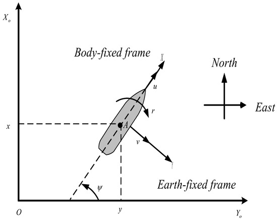
Figure 1.
Earth-fixed and body-fixed coordinate frames of a USV.
3.2. Design of Virtual Velocities
Usually, the aim of trajectory tracking control is to make the actual trajectory follow the reference trajectory by adjusting the controller according to the position error. In order to construct the Lyapunov function according to the position error equation and the design, a suitable control expression to satisfy the Lyapunov stability theory to achieve trajectory tracking, the actual position, and the reference position are calculated to obtain the position error equation.
where , , are the USV time-varying actual trajectory coordinates, reference trajectory coordinates, and error trajectory coordinates, respectively.
The derivation of the two sides of Equation (9) with respect to time t can be obtained.
where .
In order to devise the controller based on the dynamic equation, the virtual speed is defined as follows:
where and are positive numbers, and , .
The position error converges to when the actual velocity satisfies the defined virtual velocity. The velocity error is defined in the same way as the position error:
where . Then the velocity errors can be calculated as:
When the velocity error converges to , the position error satisfies the following expression:
Therefore, the following Lyapunov function can be defined according to the position error.
The time derivative of is
It can be seen that Inequality (16) is semi-negative definite, and the position error converges asymptotically, which means that when the speed error converges to , the position error also converges to .
3.3. Design of the USV Controller
Next, it must be ensured that the convergence of the velocity error satisfies the convergence of the position error. For the sliding mode control, a sliding mode surface is constructed according to the error, and a suitable control law is designed to ensure that the sliding mode surface satisfies the Lyapunov stability condition.
Without considering the environmental disturbances, we consider the following NTSM surfaces:
The derivative of the virtual speed can be obtained:
where , .
Then, the second derivative of is
where .
Let , then becomes .
Then, the time derivative of Equation (18) is:
Due to the USV tracking error in Equation (13), the following control inputs can be designed.
Stability Analysis of the USV Controller
Consider the following Lyapunov function for the NTSM:
By taking the first time derivative of the Lyapunov function , along with Equations (19) and (20), one can obtain
Substituting Equations (21) and (22) into Equation (24) yields
where , . Because is positively defined and is negatively defined, it can be seen that the NTSM surfaces meet the Lyapunov stability condition, which indicates that the system can reach the sliding mode surfaces from any initial position, as given in Equation (18). When the trajectory reaches the sliding mode surfaces, , , and can be obtained. That is to say, the constructed NTSM can make the velocity error converge, thus indicating the position error convergence.
3.4. Disturbance Observer
The disturbance of the external environment cannot be ignored in the actual navigation of underactuated USVs. In order to eliminate the influence of disturbances on the controller, a nonlinear disturbance observer [40] was introduced to estimate the unknown disturbances and compensate for disturbances in the controller, to achieve high-quality control of the closed-loop system.
and can take the following forms:
The nonlinear disturbance observer was constructed using Equations (26)–(28), where is an invertible matrix which can be solved for via linear matrix inequality (LMI).
The stability of the disturbance observer is proved in the next subsection. If the disturbance errors converge, then the disturbance observer is stable, and it can be used for controller design.
Proof of the Disturbance Observer
The Lyapunov function for the disturbance error is constructed as
Combining Equations (27)–(29), the following equation can be obtained:
where is the disturbance error.
Since it is assumed in this study that the perturbation changes slowly, it can be considered that . The observation error equation is obtained by combining with Equation (27).
The following inequality is constructed:
where is the positively defined matrix, and the existence of makes valid. Clearly, the disturbance observer converges exponentially, and the accuracy and speed of convergence depend on the value of .
The higher the value of , the higher the convergence speed and precision.
Let , then Inequality (33) becomes
From Equation (28), according to the Schur complement lemma, we can derive
The value of can be obtained by solving Inequality (34), and thus the unknown in Inequality (33) can be obtained.
The USV controller is redesigned to account for disturbances. The time derivative of Equation (18) is:
The surge force and yaw moment can be defined as follows:
For the stability analysis of the trajectory tracking control law under disturbances, the following Lyapunov function is constructed:
Taking the time derivative at both ends of Equation (38), and then substituting the control laws, Equations (36) and (37) yield
Since the designed disturbance observer converges, Equation (39) can be rewritten as
where , , and . In a similar way, the designed NTSM control law can converge to b in a finite period of time.
To eliminate the chattering phenomenon arising from the discontinuous sign function, the following saturation function is used to replace the sign function,
where and .
4. Simulations and Discussion
In this section, the USV model, controller, and disturbance observer are written in MATLAB functions based on the Simulink environment, and numerical simulations are performed using a variable step size to verify the effectiveness of the designed control strategy. First, the trajectory tracking performance was validated under ideal conditions. Under non-ideal conditions, the disturbance caused by the external environment is unknown and cannot be directly measured. Next, constant environmental disturbances were introduced, disturbance observers were used to measure disturbances, and NTSM controllers with disturbance compensation were employed to achieve trajectory tracking. The inclusion of constant environmental disturbances alone is insufficient to prove the observation effect of the disturbance observer for unknown disturbances and cannot reflect real-world scenarios. Therefore, time-varying environmental disturbances were introduced to verify the compensation for the disturbance and the trajectory tracking. The model parameters of the USV can be found in [41] and are shown in Table 1.

Table 1.
Hydrodynamic parameters of the REMUS AUV.
The controller’s control performance was verified using the following two trajectories under three different conditions.
4.1. Straight-Line Trajectory Simulation
The following straight-line trajectory was used in the simulation:
Case 1 was without environment disturbances.
Case 2 had constant environmental disturbances, where the following disturbances were chosen:
Case 3 had time-varying environmental disturbances, where the following form of the disturbances was used:
The initial position of the USV was , the initial velocity was , the initial value of was 0.5, and , . For the disturbance observer, the parameters and were chosen. The parameters used to design the NTSM controller based on Equations (37) and (42) are listed in Table 2.
Table 2.
Controller parameters for the straight-line trajectory.
Figure 2a shows the straight-line trajectory curve of the underactuated USV without any disturbances, with steady disturbances , and with time-varying disturbances . The solid line is the reference trajectory curve, and the three dotted lines are the actual trajectory curves of the USV under different conditions. From the figure, it can be seen that with the control strategy proposed in this paper, the USV is able to overcome the influence of external environmental disturbances and track a straight trajectory in three different cases. Figure 2b represents the curves of the USV in the plane, the surge (axis direction), and the sway (axis direction) positions over time. It can better reflect the change of the trajectory over time. It can be seen from the figure that the USV tracks the reference trajectory in a very short period of time and maintains stable tracking at all times. Since the USV is underactuated and has no thrusters in the sway direction, it can be seen from the figure that it takes more time to track the reference curve in the axis direction than in the axis direction.
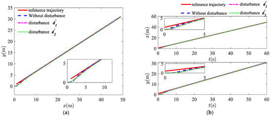
Figure 2.
Straight-line trajectory tracking in three cases: (a) trajectory tracking in the xy plane; (b) trajectory tracking in the x-axis and the y-axis directions.
Figure 3 shows the observed curves and the observed error curves of the nonlinear perturbation observer for two different environmental perturbations and . It can clearly be seen in Figure 3a,b that the disturbance observer is able to quickly approximate the external unknown environmental disturbances. Figure 3c,d show the errors between the actual disturbances and the observed values, showing that the designed disturbance observer for both the constant disturbances and the time-varying external environmental disturbances is able to estimate the actual disturbance values quickly and accurately. Therefore, the disturbance values observed by the disturbance observer can be used to replace the disturbances caused by wind, waves, and currents in the external environment, thus improving the robustness of the system.
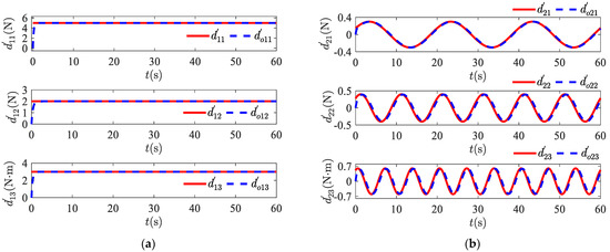
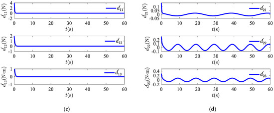
Figure 3.
Disturbance observer simulation results: (a) actual values and observed values for constant disturbances; (b) actual values and observed values for time-varying disturbances; (c) constant disturbance errors; (d) time-varying disturbance errors.
Figure 4a,b show the actual position variation curves and the actual velocity variation curves of the USV, respectively, in the three cases. As can be seen from the figures, the position and speed curves under the effect of disturbances have the same pattern as those without disturbances, which further indicates that the controller has an excellent anti-disturbance capability. Figure 4c,d show the position error variation curve and velocity error variation curve of the USV, respectively, in the three cases. The position and velocity error curves more clearly reflect the USV tracking reference trajectory. As shown in the figures, there is a large error at the initial stage of navigation, but after a period of intervention both the position error and velocity error approach zero, which shows that the designed controller can effectively track the linear reference trajectory. Figure 5 shows the variation curves for the surge force and yaw moment. The output curve of the controller becomes a smooth curve, maintaining tracking with a short adjustment time.
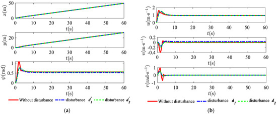
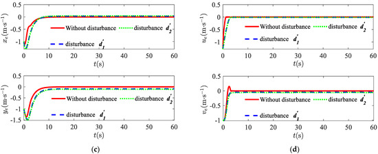
Figure 4.
Position and velocity curves: (a) the actual position of USV in three cases; (b) the actual velocity of USV in three cases; (c) position tracking errors in three cases; (d) velocity tracking errors in three cases.
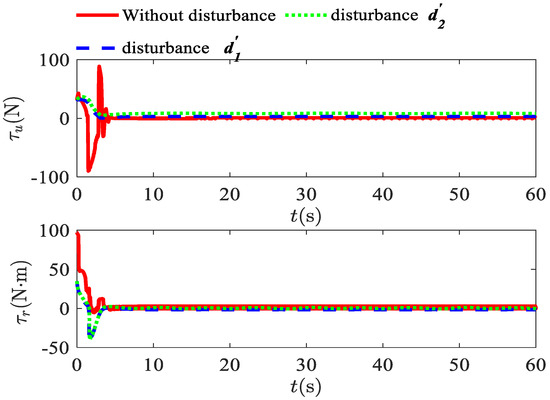
Figure 5.
Surge force and yaw moment in three cases.
4.2. Circular Trajectory Simulation
The following circular trajectory was chosen for the circle trajectory simulations:
Case 1 was without environment disturbances.
Case 2 had constant environment disturbances , chosen as described in Equation (44).
Case 3 had time-varying environment disturbances , as described in Equation (45).
The initial conditions of the USV and the parameters of the disturbance observer were consistent with the parameters of the linear trajectory. The parameters used to design the NTSM controller based on Equations (37) and (42) are listed in Table 3.
Table 3.
Controller parameters for the circular trajectory.
Figure 6, Figure 7 and Figure 8 show the simulation curves for the circular trajectory. From the simulation results, it can be seen that for circular trajectories in three different cases, the designed control strategy enabled the USV to overcome the external disturbances to achieve tracking on circular trajectories. Figure 6a illustrates the overall trajectory tracking of the USV in the plane. Figure 6b presents the trajectory tracking curves over time in the surge (axis) and sway (axis) directions. The observation approximation effect and estimation errors are presented in Figure 3. Figure 7a shows the six state curves including position and velocity curves during the USV navigation. It can be observed in Figure 7b that, in the simulations with time-varying disturbances, the velocity curve has smaller fluctuations compared with the other two cases. This is because there is a certain error in the observed effect of the disturbance observer for the time-varying disturbances. From the position error curve and velocity error curve in Figure 7c,d, it can be seen that the error has a good convergence pattern, which means that the USV can achieve circular trajectory tracking. Figure 8 shows the variation curves for the surge force and yaw moment.
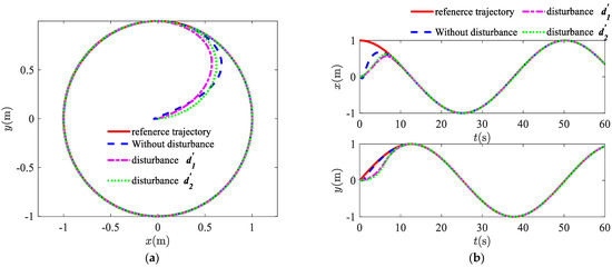
Figure 6.
Circular trajectory tracking in three cases: (a) trajectory tracking in the x-y plane; (b) trajectory tracking in the x-axis and the y-axis directions.
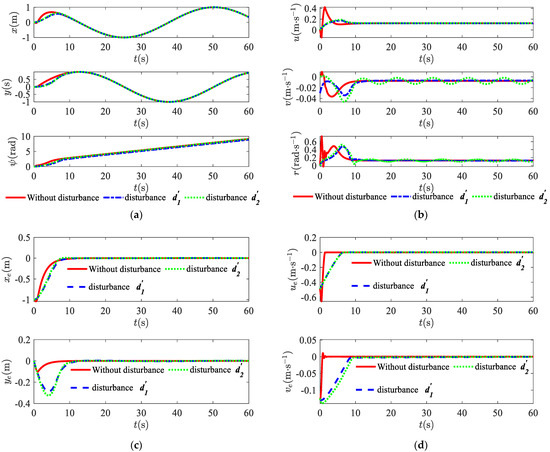
Figure 7.
Position and velocity curves: (a) the actual position of USV in three cases; (b) the actual velocity of USV in three cases; (c) position tracking errors in three cases; (d) velocity tracking errors in three cases.
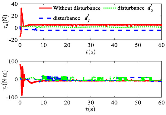
Figure 8.
Surge force and yaw moment in three cases.
The simulations for the straight-line and circular trajectories indicate that the designed control strategy is able to overcome external environmental disturbances in the process of trajectory tracking.
5. Conclusions
In this paper, an NTSM controller was designed for the trajectory tracking problem of underactuated USVs in the absence of disturbance, then a nonlinear disturbance observer was devised to observe wind, wave, and current disturbances. The designed control strategy was strictly proved to be asymptotically stable using the Lyapunov stability theory. Finally, the NTSM and the nonlinear disturbance observer were combined, and the output of the disturbance observer was used to replace the actual environmental disturbance. The following conclusions are drawn from the theoretical analysis and numerical simulations of circular and linear trajectories:
- (1)
- The trajectory tracking results were obtained by Simulink numerical simulation using the parameters of an existing USV model. In the case of no disturbance, the errors in the linear trajectory and circular trajectory speeds converged to zero quickly while the error in the position results converged to zero within 10 s to follow the the predefined trajectory, which verifies the feasibility of the controller.
- (2)
- Numerical simulations of both constant and time-varying external environmental wind, wave, and current disturbances were performed, and estimates were obtained with the designed disturbance observer. In both cases, the disturbance errors converged rapidly to a value close to zero, indicating the capability of the disturbance observer with regard to external disturbances.
- (3)
- With constant and time-varying disturbances, the USV completed the trajectory tracking task within 10 s, and the errors in velocity and position were very close to zero. The robustness of the system was improved by incorporating a disturbance observer to estimate environmental disturbances and compensating for external disturbances in the controller.
Author Contributions
Conceptualization, D.X. and X.Z.; data curation, Z.L. and L.Y.; formal analysis, Z.L.; funding acquisition, D.X. and X.Z.; methodology, D.X., L.Y. and L.H.; resources, D.X. and X.Z.; writing—original draft, D.X. and Z.L.; writing—review and editing, D.X. and X.Z. All authors have read and agreed to the published version of the manuscript.
Funding
This research was supported by the Science Fund Project of Heilongjiang Province (LH2021E087) and the National Natural Science Foundation of China (51779055).
Institutional Review Board Statement
Not applicable.
Informed Consent Statement
Not applicable.
Data Availability Statement
Not applicable.
Conflicts of Interest
The authors declare no conflict of interest.
References
- Jalving, B.; Kristensen, J.; Størkersen, N. Program philosophy and software architecture for the HUGIN seabed surveying UUV. IFAC Proc. Vol. 1998, 31, 211–216. [Google Scholar] [CrossRef]
- Asakawa, K.; Kojima, J.; Kato, Y.; Matsumoto, S.; Kato, N. Autonomous underwater vehicle AQUA EXPLORER 2 for inspection of underwater cables. In Proceedings of the 2000 International Symposium on Underwater Technology, Tokyo, Japan, 26 May 2000; pp. 242–247. [Google Scholar]
- Børhaug, E.; Pavloc, A.; Panteley, E.; Pettersec, K.Y. Straight line path following for formations of underactuated marine surface vessels. IEEE Trans. Control Syst. Technol. 2010, 19, 493–506. [Google Scholar] [CrossRef]
- Gafurov, S.A.; Klochkov, E.V. Autonomous unmanned underwater vehicles development tendencies. Procedia Eng. 2015, 106, 141–148. [Google Scholar] [CrossRef] [Green Version]
- Khalid, M.; Ullah, Z.; Ahmad, N.; Arshad, M.; Jan, B.; Cao, Y.; Adnan, A. A survey of routing issues and associated protocols in underwater wireless sensor networks. J. Sens. 2017, 2017, 7539751. [Google Scholar] [CrossRef]
- Fossen, T.I. Handbook of Marine Craft Hydrodynamics and Motion Control, 1st ed.; Wiley: Hoboken, NJ, USA, 2011. [Google Scholar]
- Hwang, C.L.; Chiang, C.C.; Yeh, Y.W. Adaptive Fuzzy Hierarchical Sliding-Mode Control for the Trajectory Tracking of Uncertain Underactuated Nonlinear Dynamic Systems. IEEE Trans. Fuzzy Syst. 2014, 22, 286–299. [Google Scholar] [CrossRef]
- Xu, H.T.; Fossen, T.I.; Guedes Soares, C. Uniformly semiglobally exponential stability of vector field guidance law and autopilot for path-following. Eur. J. Control 2020, 53, 88–97. [Google Scholar] [CrossRef]
- Liu, S.Q.; Sang, Y.J.; Whidborne, J.F. Adaptive sliding-mode-backstepping trajectory tracking control of underactuated airships. Aerosp. Sci. Technol. 2020, 97, 1–13. [Google Scholar] [CrossRef]
- Xu, H.T.; Rong, H.; Gueds Soares, C. Use of AIS data for guidance and control of path-following autonomous vessels. Ocean Eng. 2019, 194, 106635. [Google Scholar] [CrossRef]
- Lecce, N.D.; Laschi, C.; Bibuli, M.; Bruzzone, G.; Zereik, E. Neural dynamics and sliding mode integration for the guidance of unmanned surface vehicles. In Proceedings of the Oceans 2015—Genova, Genova, Italy, 18–21 May 2015; pp. 1–6. [Google Scholar]
- Chen, L.P.; Zhou, B.B.; Mao, R.Q.; Wu, K.Q. Adaptive neural network trajectory tracking control for an underactuated unmanned surface vehicle. In Proceedings of the IEEE 9th Annual International Conference on CYBER Technology in Automation, Control, and Intelligent Systems, Suzhou, China, 29 July–2 August 2019; pp. 295–300. [Google Scholar]
- Nodland, D.; Zargarzadeh, H.; Jagannathan, S. Neural Network-Based Optimal Adaptive Output Feedback Control of a Helicopter UAV. IEEE Trans. Neural Netw. Learn. Syst. 2013, 24, 1061–1073. [Google Scholar] [CrossRef]
- Loría, A. Observers are Unnecessary for Output-Feedback Control of Lagrangian Systems. IEEE Trans. Autom. Control 2016, 61, 905–920. [Google Scholar] [CrossRef] [Green Version]
- Yan, Z.P.; Gong, P.; Zhang, W.; Wu, W.H. Model predictive control of autonomous underwater vehicles for trajectory tracking with external disturbances. Ocean Eng. 2020, 217, 107884. [Google Scholar] [CrossRef]
- Shen, C.; Shi, Y. Distributed implementation of nonlinear model predictive control for AUV trajectory tracking. Automatica 2020, 115, 108863. [Google Scholar] [CrossRef]
- Liang, H.J.; Li, H.P.; Xu, D.M. Nonlinear Model Predictive Trajectory Tracking Control of Underactuated Marine Vehicles: Theory and Experiment. IEEE Trans. Ind. Electron. 2021, 68, 4238–4248. [Google Scholar] [CrossRef]
- Xu, H.T.; Oliveira, P.; Guedes Soares, C. L1 adaptive backstepping control for path-following of underactuated marine surface ships. Eur. J. Control 2021, 58, 357–372. [Google Scholar] [CrossRef]
- Zou, A.-M. Finite-Time Output Feedback Attitude Tracking Control for Rigid Spacecraft. IEEE Trans. Control Syst. Technol. 2014, 22, 338–345. [Google Scholar] [CrossRef]
- Wang, N.; Deng, Z.C. Finite-Time Fault Estimator Based Fault-Tolerance Control for a Surface Vehicle With Input Saturations. IEEE Trans. Ind. Inform. 2020, 16, 1172–1181. [Google Scholar] [CrossRef]
- Zhang, L.; Huang, B.; Liao, Y.L.; Wan, B. Finite-Time Trajectory Tracking Control for Uncertain Underactuated Marine Surface Vessels. IEEE Access 2019, 7, 102321–102330. [Google Scholar] [CrossRef]
- Liang, X.; Qu, X.R.; Hou, Y.H.; Li, Y.; Zhang, R.B. Finite-time unknown observer based coordinated path-following control of unmanned underwater vehicles. J. Franklin. Inst. 2021, 358, 2703–2721. [Google Scholar] [CrossRef]
- Fan, Y.S.; Liu, B.W.; Wang, G.F.; Mu, D.D. Adaptive Fast Non-Singular Terminal Sliding Mode Path Following Control for an Underactuated Unmanned Surface Vehicle with Uncertainties and Unknown Disturbances. Sensors 2021, 21, 7454. [Google Scholar] [CrossRef]
- Swaroop, D.; Hedrick, J.K.; Yip, P.P.; Gerdes, J.C. Dynamic surface control for a class of nonlinear systems. IEEE Trans. Autom. Control 2000, 45, 1893–1899. [Google Scholar] [CrossRef] [Green Version]
- Wang, N.; Liu, Z.Z.; Zheng, Z.J.; Er, M.J. Global exponential trajectory tracking control of underactuated surface vehicles using dynamic surface control approach. In Proceedings of the 2018 International Conference on Intelligent Autonomous Systems, Singapore, 1–3 March 2018; pp. 221–226. [Google Scholar]
- Xu, J.; Wang, M.; Qiao, L. Dynamical sliding mode control for the trajectory tracking of underactuated unmanned underwater vehicles. Ocean Eng. 2015, 105, 54–63. [Google Scholar] [CrossRef]
- Zhao, Y.S.; Sun, X.J.; Wang, G.F.; Fan, Y.S. Adaptive Backstepping Sliding Mode Tracking Control for Underactuated Unmanned Surface Vehicle With Disturbances and Input Saturation. IEEE Access 2021, 9, 1304–1312. [Google Scholar] [CrossRef]
- Fu, M.Y.; Yu, L.L. Finite-time extended state observer-based distributed formation control for marine surface vehicles with input saturation and disturbances. Ocean Eng. 2018, 159, 219–227. [Google Scholar] [CrossRef]
- Huang, C.F.; Zhang, X.K.; Zhang, G.Q. Improved decentralized finite-time formation control of underactuated USVs via a novel disturbance observer. Ocean Eng. 2019, 174, 117–124. [Google Scholar] [CrossRef]
- Wang, N.; Sun, Z.; Yin, J.C.; Zou, Z.J.; Su, S.F. Fuzzy unknown observer-based robust adaptive path following control of underactuated surface vehicles subject to multiple unknowns. Ocean Eng. 2019, 176, 57–64. [Google Scholar] [CrossRef]
- Kurtoglu, D.; Bidikli, B.; Tatlicioglu, E.; Zergeroglu, E. Periodic disturbance estimation based adaptive robust control of marine vehicles. Ocean Eng. 2021, 219, 108351. [Google Scholar] [CrossRef]
- Yang, H.L.; Deng, F.; He, Y.; Jiao, D.M.; Han, Z.L. Robust nonlinear model predictive control for reference tracking of dynamic positioning ships based on nonlinear disturbance observer. Ocean Eng. 2020, 215, 107885. [Google Scholar] [CrossRef]
- Yu, H.M.; Guo, C.; Shen, Z.P.; Yan, Z.P. Output Feedback Spatial Trajectory Tracking Control of Underactuated Unmanned Undersea Vehicles. IEEE Access 2020, 8, 42924–42936. [Google Scholar] [CrossRef]
- Chen, L.P.; Cui, R.X.; Yang, C.G.; Yan, W.S. Adaptive Neural Network Control of Underactuated Surface Vessels With Guaranteed Transient Performance: Theory and Experimental Results. IEEE Trans. Ind. Electron. 2020, 67, 4024–4035. [Google Scholar] [CrossRef] [Green Version]
- Liu, K.; Wang, R.J.; Wang, X.D.; Wang, X.X. Anti-saturation adaptive finite-time neural network based fault-tolerant tracking control for a quadrotor UAV with external disturbances. Aerosp. Sci. Technol. 2021, 115, 106790. [Google Scholar] [CrossRef]
- Zou, L.P.; Liu, H.T.; Tian, X.H. Robust Neural Network Trajectory-Tracking Control of Underactuated Surface Vehicles Considering Uncertainties and Unmeasurable Velocities. IEEE Access 2021, 9, 117629–117638. [Google Scholar] [CrossRef]
- Yu, S.H.; Yu, X.H.; Shirinzadeh, B.; Man, Z.H. Continuous finite-time control for robotic manipulators with terminal sliding mode. Automatica 2005, 41, 1957–1964. [Google Scholar] [CrossRef]
- Bu, X.H.; Liang, J.Q.; Wang, S.; Yu, W. Robust guaranteed cost control for a class of nonlinear 2-d systems with input saturation. Int. J. Control Autom. 2020, 18, 513–520. [Google Scholar] [CrossRef]
- Korotkin, A.I. Added Masses of Ship Structures, 1st ed.; Morwest Publishers: St. Petersburg, Russia, 2007. [Google Scholar]
- Yang, Y.; Du, J.L.; Liu, H.B.; Guo, C.; Abraham, A. A trajectory tracking robust controller of surface vessels with disturbance uncertainties. IEEE Trans. Control Syst. Technol. 2013, 22, 1511–1518. [Google Scholar] [CrossRef]
- Elmokadem, T.; Zribi, M.; Youcef-Toumi, K. Terminal sliding mode control for the trajectory tracking of underactuated Autonomous Underwater Vehicles. Ocean Eng. 2017, 129, 613–625. [Google Scholar] [CrossRef]
Publisher’s Note: MDPI stays neutral with regard to jurisdictional claims in published maps and institutional affiliations. |
© 2022 by the authors. Licensee MDPI, Basel, Switzerland. This article is an open access article distributed under the terms and conditions of the Creative Commons Attribution (CC BY) license (https://creativecommons.org/licenses/by/4.0/).