Article

Three-Dimensional Modeling of the Xichang Crust in Sichuan, China by Machine Learning

1
Key Laboratory of Computational Geodynamics, University of Chinese Academy of Sciences, Beijing 100049, China
2
Chongqing Earthquake Agency, Chongqing 401147, China
3
Beijing Baijiatuan Earth Science National Observation and Research Station, Beijing 100095, China
4
Institute of Geophysics, China Earthquake Administration, Beijing 100081, China
*
Author to whom correspondence should be addressed.
Appl. Sci. 2022, 12(6), 2955; https://doi.org/10.3390/app12062955
Submission received: 31 January 2022 / Revised: 3 March 2022 / Accepted: 7 March 2022 / Published: 14 March 2022
(This article belongs to the Special Issue Integration of Methods in Applied Geophysics)

Abstract

:
Seismicity and distribution of earthquakes can provide active fault structural information on the crust at a regional scale. The morphology of faults can be derived from the epicentral distribution of micro-earthquakes. In this study, we combined both the relocated earthquake catalogue and related preliminary geophysical information for 3D modeling of the crust in the Xichang area, Sichuan province, China. The fault morphology and deep crustal structure were automatically extracted by the machine learning approach, such as the supervised classification and cluster analysis methods. This new 3D crustal model includes the seismic velocity distribution, fault planes in 3D and 3D seismicity. There are many earthquake clusters located in the folded basement and low-velocity zone. Our model revealed the topological relation between the folded basement and faults. Our work show the crustal model derived is supported by the earthquake clusters which in turn controls the morphological characteristics of the crystalline basement in this area. Our use of machine learning techniques can not only be used to predict the refined fault geometry, but also to combine the seismic velocity structure with the known geological information. This 3D crustal model can also be used for geodynamic analysis and simulation of strong motionseismic waves.

1. Introduction

In recent years, a large number of high-precision observation arrays have been deployed in Sichuan and Yunnan provinces with the support of the China Seismic Experimental Site (CSES). The accuracy of seismic location and the inversion method of velocity structure was greatly improved [1] based on enhancing the microseismic monitoring capability in this region [2]. The research on fault activity has been greatly improved [3,4,5]. At the same time, fruitful scientific research achievements have been produced, such as precise location data, focal mechanism solutions [6,7], and velocity structure models based on different methods and data sources [8,9,10,11,12,13,14,15,16]. In addition, there has been a good attempt to study local engineering geological conditions by integrating multi-source geophysical data [17]. However, the crustal medium structure model used for simulating numerically large-scale regional deformations is relatively simple, which cannot well-reflect the morphological characteristics of actual crustal medium structure, and affects the reliability of simulation results [18,19]. Therefore, comprehensively utilizing the existing scientific research achievements and automatically establishing a more realistic crustal medium structure model for later model analysis and geophysical field simulation has become an urgent scientific research task to be solved.
With the increase in station density, observation accuracy improves, and the data volume and complexity are significantly enhanced. The traditional data processing methods are difficult to process the current observation data efficiently, and some Machine Learning (ML) algorithms have been widely used in Geoscience [20,21]. For example, automatic detection of rupture using source location [22], earthquake relocation [23], automatic acquisition and application of source mechanism [24,25], seismic probabilistic hazard analysis [26], fault geometry based on source information [27,28,29,30], etc. In addition, 3D visualization technology has also been deeply applied in structural geology, fault plane fitting, and the 3D structure of the lithosphere [31]. However, relatively few studies on automatic modeling are based on multiple data [4,5]. Therefore, we plan to construct a crustal framework by combining velocity structure and relocated earthquake catalogue and related geophysical prior information. Then we will refine the crustal medium structure by local refinement with a combination of fault model and source model. Finally, we integrate the multi-source model is by generating the crustal medium structure model, This geometric model will then be used for numerical simulation of seismic wave propagation.

2. Data and Methods

2.1. Data

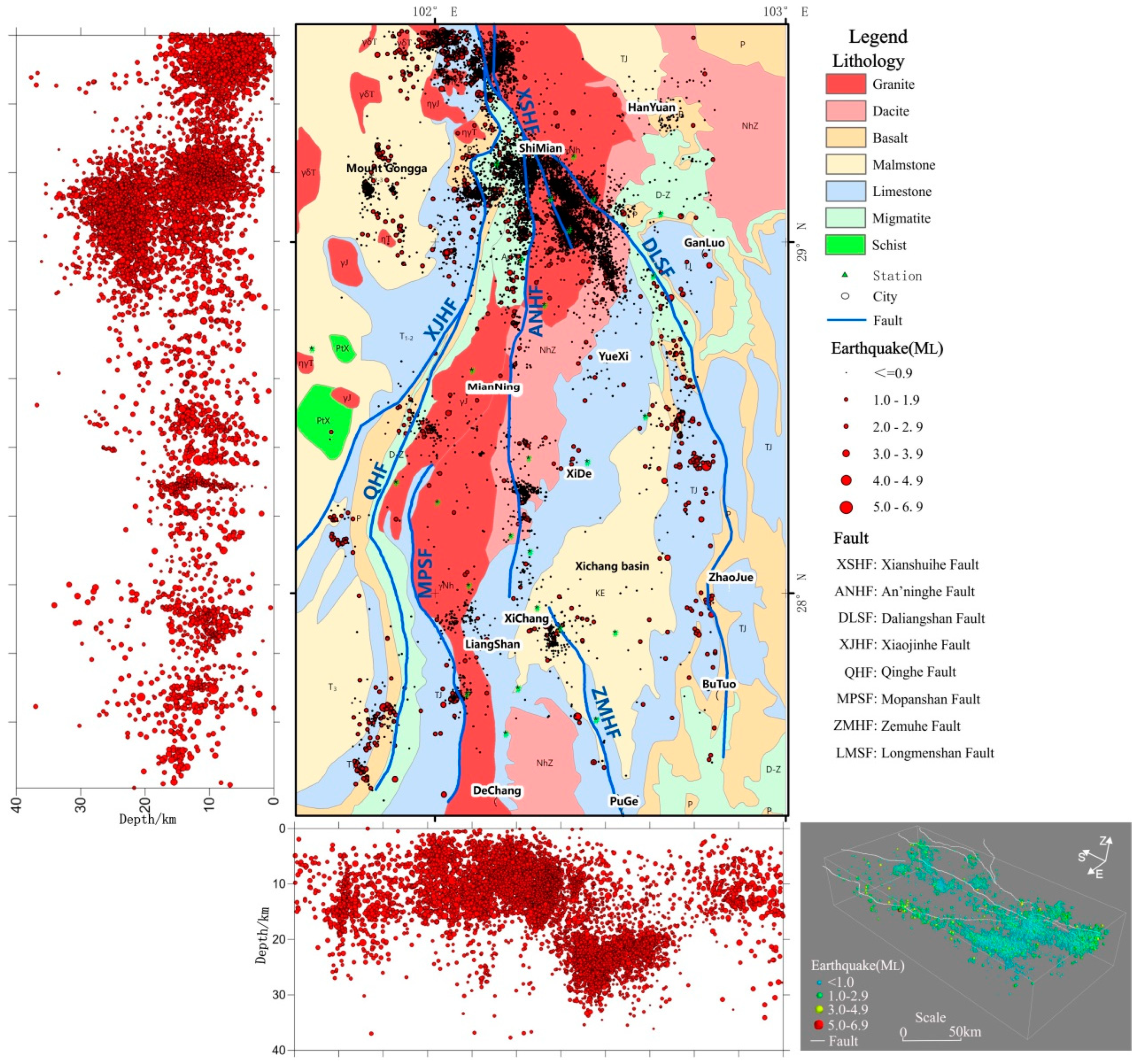
2.1.1. Seismotectonic Setting

The Xichang area is located in the middle of the Kangdian earth’s axis, at the junction of the east and west tectonic units in China, and the rhomboid block region’s core Xianshuihe and Xiaojiang fault system [32,33]. Due to the complex seismogenic structure and dynamic mechanism, this region has become important for studying intracontinental deformation. Large fault zones such as the Anninghe fault zone, Xianshuihe fault zone, and Daliangshan fault zone are mainly developed in this region with strong historical seismic activity [34]. Multi-stage magmatic rocks, metamorphic rocks, and sedimentary rocks are in contact, resulting in extremely complex tectonic and geological conditions [35]. The density and quality of the regional seismic network have been greatly improved in recent decades. Many teams have deployed dense arrays with different scales and station spacing. With the constant improvement of the precision and quality of observation data, more and more fundamnetal investigations are focused on the fault block and seismicity in this area [36,37], sliding rate of active faults [38,39], motion mode [40], structural characteristics [40,41], focal mechanism [7]. Therefore, we have now a great variety of geophysical and geological results thus providing an accurate constraint for the modeling of crustal dynamics in the Xichang area.

2.1.2. Earthquake Catalogue
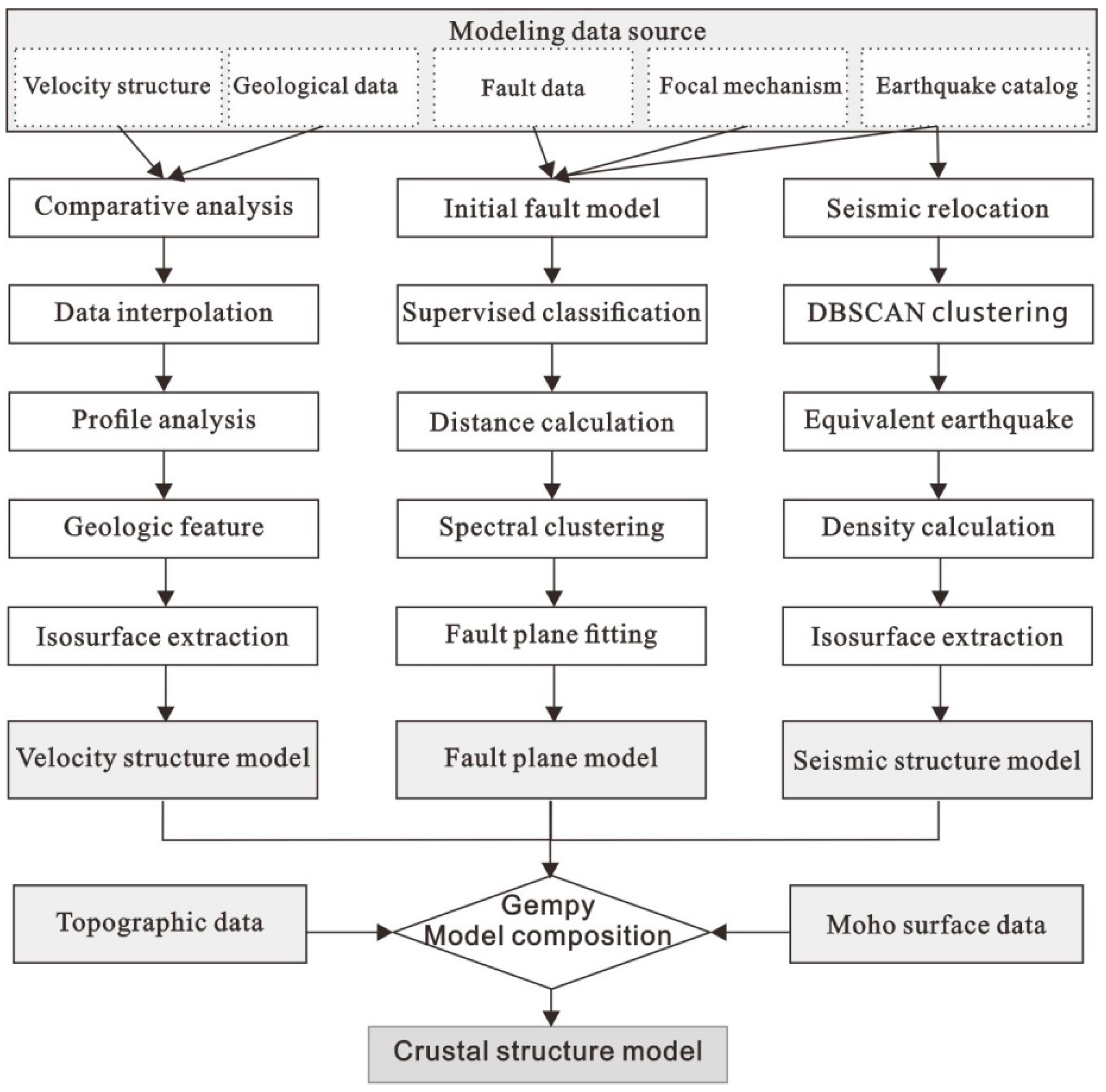
In 2012, The Institute of Geophysics of China Earthquake Administration deployed a high-density and broadband mobile seismic array in Luding-Mianning-Xichang along the Anninghe fault zone to monitor the deep seismic activity behavior. It evaluated the detection ability of the array for microearthquakes at different depths [2] and seismic activity parameters [42]. This campaign provides reliable data sources and parameter support for our quantitative approach. We have selected 9338 earthquakes monitored in this area from 2013 to 2019 as samples to conduct precise relocation. The magnitude (ML) range is −2.0 to 6.9. Combined with the characteristics of tectonic faults and lithology distribution, it is suggested that (Figure 1), except for the granite body in the Shimian area cut by the Daliangshan fault, the other faults are distributed along the boundary of the magmatic body or the Xichang basin, obviously constrained by the geometric framework of the basement. Earthquakes in this region are mainly distributed in clusters along intrusive granitic rocks and deep fault zones, especially in areas with complex fracture structures, such as the Shimian area. Along this profile, the seismic clusters also have good stratification characteristics. Most earthquakes are concentrated in the 5–20 km depth range, while the clusters in the depth range of 20–35 km are also found at fault intersections.

2.2. Methods

The traditional geophysical modeling method is to establish a relationship between velocity structure and geological body based on a large number of borehole data, seismic profile, magnetotelluric, etc. [43]. First, based on the above multi-source data, a reliable velocity structure model suitable for modeling was selected through comparative analysis of different velocity structure model results. The rock mass structure and layer structure were extracted to establish a regional crustal medium framework model combined with geological evolution data and velocity structure characteristics. Secondly, the fault initialization model is established based on the fault data on the surface, fault initial model data, and focal mechanism solution provided by the Sichuan–Yunnan experiment site. The relocated earthquake catalog established a complex fault model with a more fine structure using supervised classification, cluster analysis, and other machine learning algorithms to extract morphological fault features. Thirdly, combined with the seismic precision location data, the equivalent seismic energy particles were obtained by using the magnitude-energy conversion relationship, and the seismic energy clusters were obtained by using the unsupervised clustering ML method. The kernel density of the energy clusters was calculated respectively, and the density isosurfaces were extracted to obtain the source structure model. At last, based on the above three models, We use the Gempy library (https://www.gempy.org/, accessed on 30 January 2022) for model calculation, and the crustal medium structure model was generated. From this we derive the geometric model to be used for numerical simulation of seismic waves. The complete workflow is displayed in Figure 2.

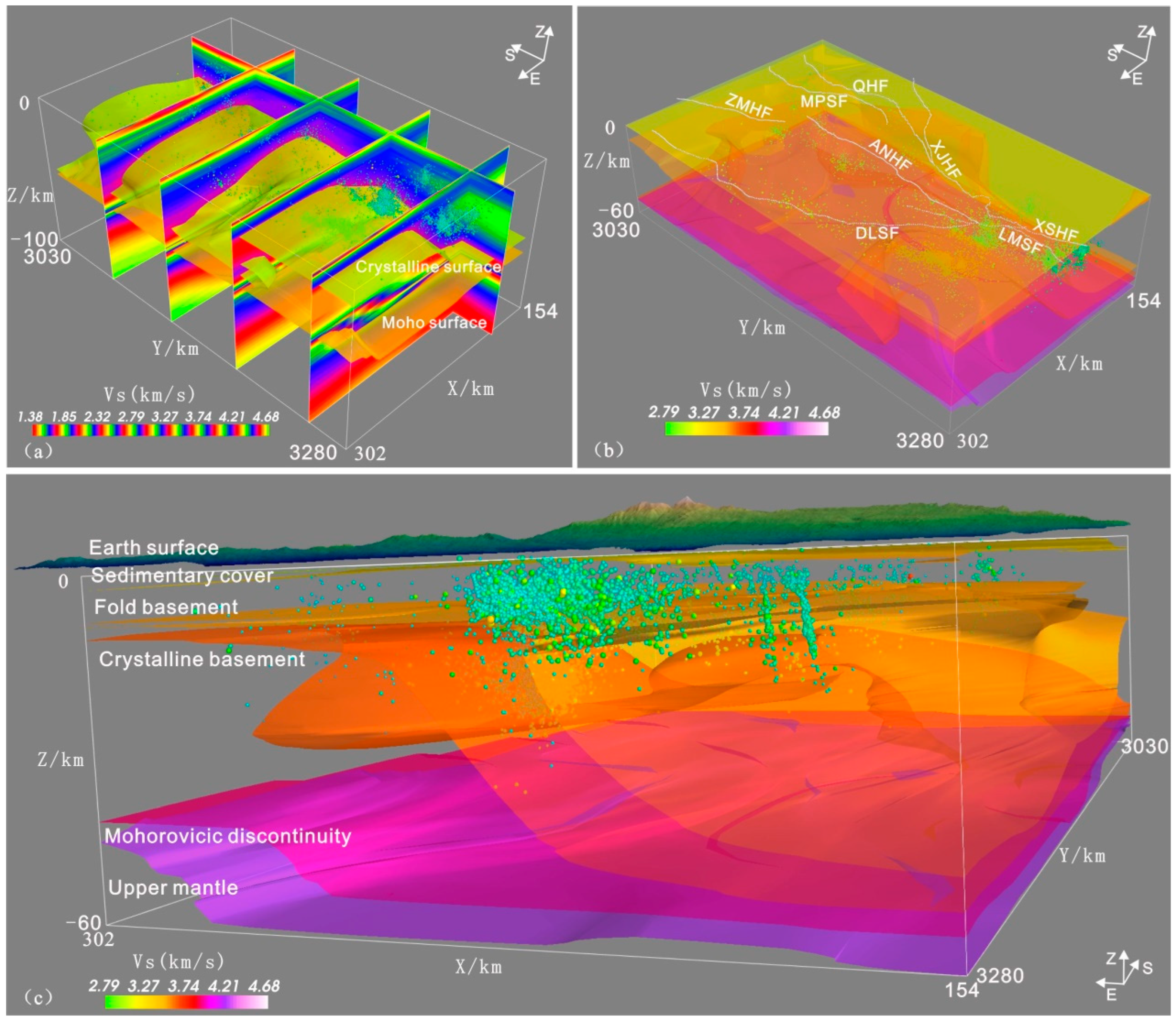
3. Velocity Structure Model

Seismic tomography has now been proved very powerful tools for studying the three-dimensional velocity structure at different scales in the earth [44,45,46]. At present, the commonly used methods include body wave tomography, surface wave tomography, receiver function, joint inversion, etc. With the significant improvement of the density and quality of the regional seismic network, many velocity structure models have been produced [8,9,10,11,12,13,14,15,16]. However, due to the inherent uncertainty of the model and the different sensitivity of different data types and inversion methods, the inversion results also have some differences. The comparative analysis of different velocity models (Table 1) found that they are generally consistent in large-scale characteristics. It can study block structure, high-speed anomaly body, and Moho surface in a large area. In this study, the model with high horizontal/vertical resolution calculated by Shen et al. (2016) [12] was selected. In order to prevent the non-uniformity of data points on the profile and distortion of interpolation result, we carried out layer interpolation based on different depths to obtain the distribution characteristics of velocity anomaly regions at different depths. Afterwards, the three-dimensional matrix data were superimposed to provide better constraints for the model, and the crustal medium frame model of this region was established for later geological modeling.
Figure 3a shows the profile characteristics of the S wave velocity structure. By color standard processing, we enhanced the display of the crustal structure. We can conclude: (1) The shallow strata with wave velocity between 1.28 km/s and 2.8 km/s have great velocity variation and shallow burial depth, consistent with the relief of Xichang Basin and relate to the boundary of the basin. (2) The velocity of 2.8–3.2 km/s cover the whole region with the gentle change, reflecting the distribution characteristics of sedimentary cover on the shallow surface, which may be Precambrian metamorphic sedimentary rocks or igneous rocks. (3) Earthquakes mostly occur in the blue region where the wave velocity structure is 3.2–3.6 km/s. The geometric morphology of this region is consistent with the folded basement of geological history. We see the presence of magmatic rocks and shallow metamorphic rocks with brittle quality and low hardness. (4) The red region with wave velocity structure in the range of 3.6–3.8 km/s has a certain uplift feature along the N-S direction in the middle, which is relatively consistent with the exposed position of the Kangdian axis and the surface granites. It is an anomalous area with high wave velocity and a hard Crystalline basement. Beneath Shimian, the rock mass is broken and staggered, resulting in many earthquakes. (5) The velocity of 3.8–4.2 km/s changes rapidly and presents discontinuity distribution, which may be Moho. In addition, on the west side of Xianshuihe, a low-velocity body appears within the Folded basement, which may be a weak mechanical zone formed by crustal compression and thickening. There are also many earthquakes in the vicinity of this low-velocity body. Given the above characteristic velocity features, the isosurfaces of 2.8 km/s, 3.2 km/s, 3.6 km/s, 3.8 km/s and 4.2 km/s are extracted respectively (Figure 3b), which have a good relationship with the distribution characteristics of faults, earthquakes, and geomorphic fluctuation features of the surface. This demonstrates the reliability of the crustal model we are dealing with (Figure 3c).

4. Morphology of Active Fault

Basement faults are usually the boundary of tectonic blocks and the potential location of moderate and strong earthquakes. In order to study more carefully the deformation characteristics, stress accumulation, and earthquake swarm migration of fault locked-in regions, we need to obtain the morphological characteristics and interactions of different faults [47]. Numerous studies have been carried out to constrain the morphological characteristics of subsurface active faults, including structural geology, topography, geomorphology, trenching, drilling, etc. The deep morphological characteristics of faults are mainly obtained by relying on the focal mechanisms, seismic tomography, and other geophysical evidences [48,49].
Since most earthquakes are distributed along the fault planes, unsupervised clustering ML technology has achieved good results in extracting the fault morphology of earthquake clusters [21]. Therefore, we focus on using structural geological data to constrain the surface morphological characteristics of a shallow fault, then uses precise seismic location, focal mechanism solution, and other research data to constrain the deep characteristics of the fault plane, so as to automatically and quickly extract the three-dimensional morphological characteristics associated with seismogenic active faults.

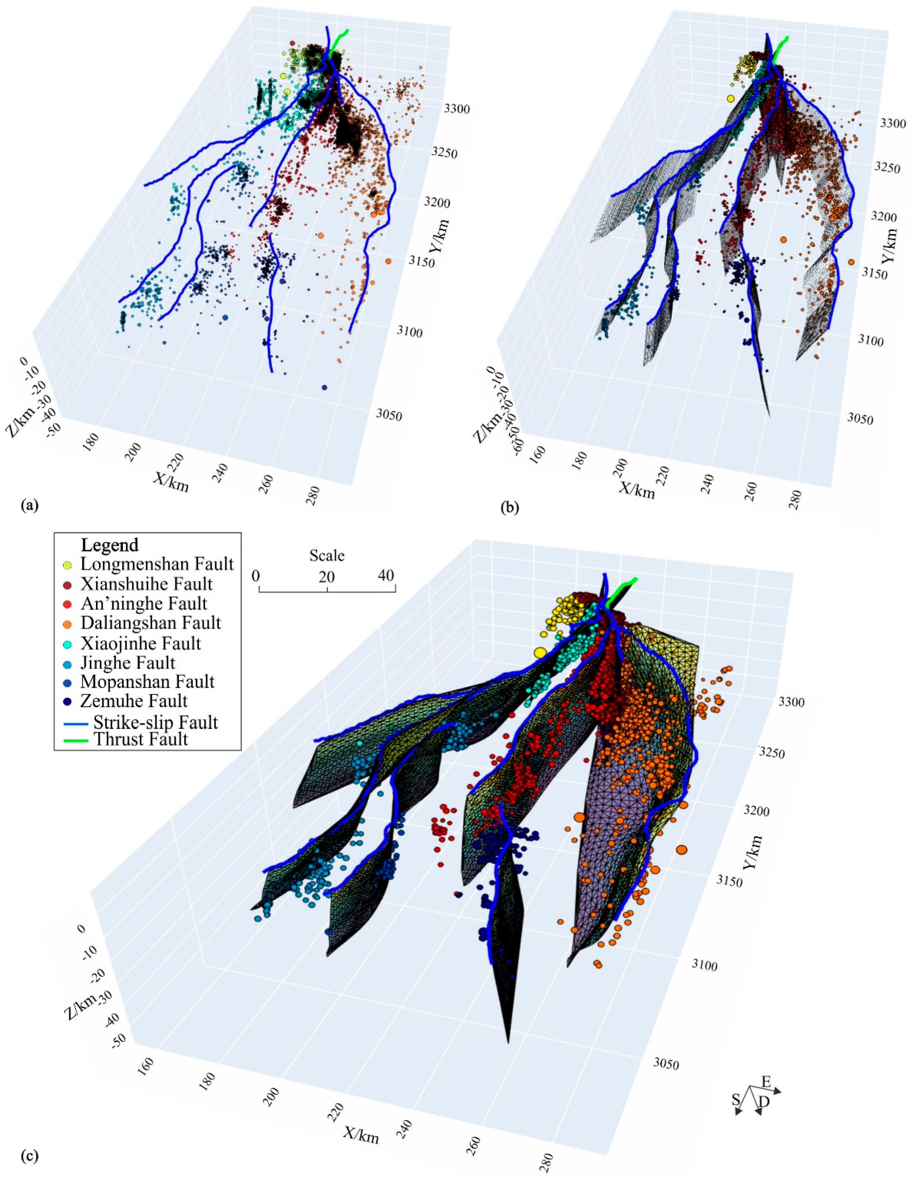
4.1. Initial Fault Model

By collecting carefully the distribution characteristics of earthquakes and the deep faults exposed in this region, we have analyzed eight deep fault zones, such as Longmenshan fault, Xianshuihe fault, Anninghe fault, Daliangshan fault, Xiaojianghe fault, Qinghe fault, Mopanshan fault, and Zemuhe fault. These faults occurred in the intermediate transition position of the Xianshuihe–Xiaojiang fault system and spread in a spindle shape near Shimian, and cut the Xichang area into multiple structural units. By referring to the basement fault data published in CSES [4], combined with the latest research results and 1:500,000 geological map of the region, the fault linear feature and occurrence information were extracted to constrain the morphological fault characteristics on the shallow surface. The details of the initial model parameters are shown in Table 2.
The focal mechanism is very important in describing geometric characteristics of faults, evaluating stress disturbance and evaluating aftershock mode. It contains the dislocation information of source rupture, and can also constrain the occurrence of a deep fault plane and distinguish the fault dislocation type. Li Jun et al. (2019) [7] analyzed the spatial distribution characteristics of the tectonic stress field in this area by using the focal mechanism solution and considering that the regional earthquake fault type is left-lateral strike-slip type. Along the Xianshuihe–Xiaojiang Fault Zone on the east boundary of the Sichuan–Yunnan block, the principal compressive stress gradually changes from NWW to NW with a clockwise rotation of about 50°. Moreover, the angle between the principal compressive stress axis and the fault strike on the east boundary remains nearly the same [7]. Because of one of the interfaces in the focal mechanism, the solution may be approximately parallel to the fault plane. Therefore, we can extract the focal mechanism solution within 5 km of the fault by means of buffer analysis, combined with the extended azimuth of the fault plane. We select the focal node information consistent with the fault plane (Table 3), and by doing so one can restrict the position of the deep fault plane.

4.2. The Geometric Features of Fault Plane

We can use a high-quality earthquake catalogue to constrain the deep structure of the fault and extract more fine morphology of the fault plane. However, the fault distribution in the Xichang area is complex, and the earthquake clusters are unevenly distributed, so it is difficult to distinguish the relationship between earthquakes and faults. Therefore, based on the previous dataset, this study established the initial model of the fault plane, used the supervised classification algorithm in machine learning to classify the earthquakes according to faults, used the machine learning unsupervised clustering technique to extract the earthquakes closely related to the fault plane, then the fault plane of the core cluster was formed. The source location was fitted by spline function to obtain the three-dimensional shape of earthquake clusters corresponding to faults and extract the morphology of fault planes. The key procedures are as follows:
(1) There is no clear correspondence between earthquake and fault. How to link earthquakes with faults has always been a key problem. The common method is buffered analysis, that is, the closer the earthquake is to the fault, the greater the possibility that the earthquake belongs to the fault. It is based on the determined fault plane. It is difficult to determine the boundary range of the distance quantitatively. However, the earthquake subordination is more complex in the adjacent or intersecting deep faults, which needs to be classified by machine learning correlation algorithm. We try to use the fault line and fault occurrence information to produce the initial fault plane model, take the fault plane node data as the training dataset, use the supervised classification of K nearest neighbor (KNN) algorithm training model, and use the seismic data as the test set to predict the faults to which the earthquake may belong, so as to classify the existing earthquakes, the classification results are shown in Figure 4a.
(2) Due to the uncertainty of earthquake location and background noise effects, the earthquakes are not strictly distributed according to the fault direction. There are often some background earthquakes between faults, which may affect the fitting accuracy of the fault plane. The spectral clustering algorithm has obvious advantages in screening seismic clusters related to the fault plane [31]. It is based on the spectral graph theory, which has the advantages of clustering in the arbitrary shape of sample space and converging to the optimal global solution compared with the traditional clustering algorithm. The closer an earthquake is to a fault line, the greater the probability related to the fault and the greater the degree of membership. The definition of distance or similarity measure usually controls the shape of the clusters. Therefore, it is necessary to calculate the distance between the earthquake and the extension direction of the fault line, the distribution direction of the fault plane, and the direction of the focal mechanism nodal plane, respectively, and establish a quantitative similarity matrix based on this. Then, the spectral clustering algorithm selected the earthquakes related to faults. In the process of spectral clustering, the number of seismic clusters and the number of iterations need to be set. After repeated experiments, the final parameters were selected as n_cluster = 5, n = 100 times. The earthquake clusters close to the fault were selected in the clustering results so that the background noise earthquakes could be better eliminated. See Figure 4b for the clustering results.
(3) After obtaining the earthquake clusters highly related to faults, they can be spatially interpolated, and the most suitable 3D fault plane can be fitted. In order to facilitate calculation, the fault plane fitting method similar to Brunsvik et al. (2021) [31] was adopted in this study, and the strike, dip, and normal direction pointing to the hanging wall of the fault plane were selected as the three coordinate axes of the local coordinate system. In order to avoid unnatural oscillations between high-order polynomial interpolation data, a bicubic spline was used to interpolate seismic sources. The spline algorithm constructs a continuous smooth piecewise polynomial. A 7 × 7 grid node (solving spline parameters of nodes) was created on the most suitable fault plane, ensuring that all the earthquake clusters are included in the node grid. The least-square method was used to invert the node parameters to minimize the distance between the source and the spline curve. The node parameters describe the third-order polynomial defined only locally around the node and finally obtain the most suitable fault model to refine the fault plane’s structure further.

5. Seismotectonic Structure
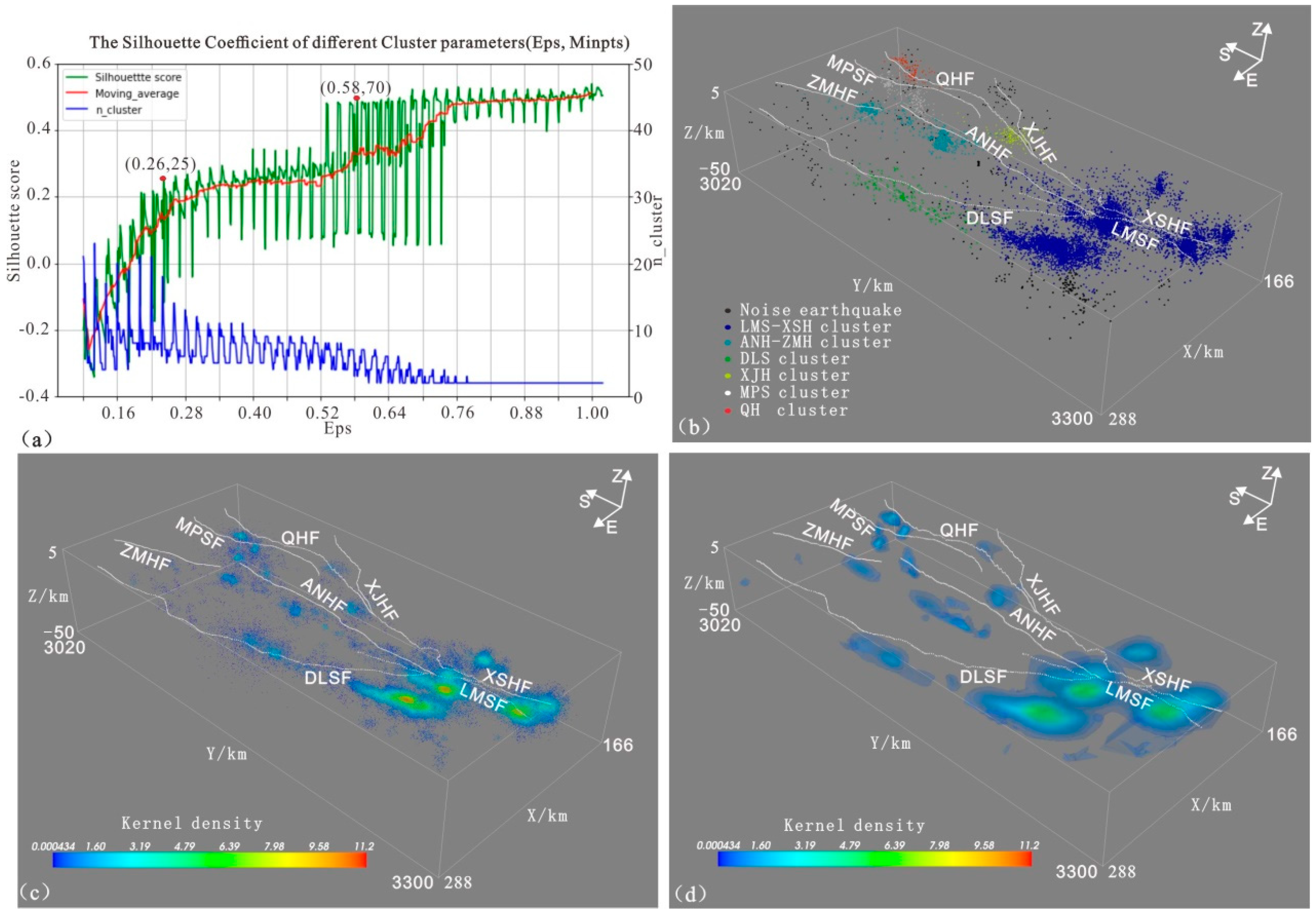
The earthquake distribution is affected by the fault location and influenced by crustal medium structures. Different shapes of earthquake clusters formed and depicted the crustal medium fracture zone, a high probability area for seismic energy release. The intersection of its extension direction and fault may be an important area for large earthquakes and new potential fractures in the future. The construction of the seismic source model is the most subjective and controversial part. In general, there is no systematic and quantitative way to accomplish this task [26]. Therefore, to further refine the geometric features of the seismic source area and fully consider the damaged areas of the crustal medium caused by the different earthquakes, this study extracted the density isosurfaces of seismic clusters to obtain the geometric features of the focal area combined with the distribution characteristics of earthquake clusters. Our source model is naturally more suitable for the observed seismicity than the models derived from other geological and seismotectonic information.

5.1. DBSCAN

The DBSCAN algorithm can describe the tightness of a sample set based on a group of neighborhoods. Two parameters (ε, MinPts) are used to describe the tightness of the sample distribution of the neighborhood. The ε describes the neighborhood distance threshold of the sample. The MinPts describes the neighborhood sample number threshold of a certain sample whose distance is ε. The biggest advantage of this algorithm is that it does not need to input the number of clusters K and can find clusters of arbitrary shape and eliminate some scattered noise events. Since the density clustering still needs to provide the distance threshold of the sample field and the number of samples, in order to achieve a better clustering effect, this study measures the rationality of clustering by Silhouette coefficient, setting the neighborhood distance range of the samples as 0.1–1 and the step length as 0.02, the threshold range of the number of seismic cluster samples as 10–100 and the step size as 5. Figure 5a shows that with the increase in test thresholds, the Silhouette coefficient also increases rapidly. The Silhouette coefficient tends to rise slowly when the neighborhood distance exceeds 0.26, and the corresponding model parameters are (ε = 0.26, MinPts = 25). However, the sample number of some earthquake clusters is small, so it is difficult to extract the corresponding source morphology. On the premise of ensuring the diversity of classification, the clustering effect is the best when the model parameters are ε = 0.58, MinPts = 70. Seven earthquake clusters were obtained, and all were distributed near the fault, which can better display the characteristics of the source structure (Figure 5b).

5.2. Seismic Energy Cluster

Due to the small number of earthquake samples, it is not conducive to describing the morphological characteristics of earthquake clusters. In addition, the seismic cluster analysis only considers the source location information but ignores the magnitude of earthquakes. As the magnitude of an earthquake increases, the energy it releases and the range of its effects increase exponentially. In order to eliminate the influence of magnitude on the shape of seismic clusters, we calculated the energy of each earthquake by the relation of magnitude and energy, which can be transformed into equivalent earthquake particles positively distributed in the source so as to describe the morphological characteristics of earthquake clusters truly. Combined with the clustering results of seismic clusters mentioned above, the equivalent seismic particles are further classified to obtain the corresponding seismic energy clusters.

5.3. Density Calculation and Isosurface Extraction

The distribution of equivalent seismic particles in the seismic energy clusters is not uniform. The more concentrated the distribution is, the greater the density is, the more concentrated the energy release is, and the greater the rupture degree of the crustal medium. The seismic energy cluster density isosurface can better describe the seismic source structure’s morphological characteristics. Therefore, in this study, the kernel density of each seismic energy cluster is calculated through Gaussian kernels. Then the isosurface is extracted to obtain more natural geometric characteristics of the source. The clusters in Figure 5c are divided into three levels according to the density marked with blue, yellow, and red, respectively. The blue delineated area is mainly the seismic cluster at the lower part of several fault zones, and the long axis direction is consistent with the fault direction. The crustal medium is relatively broken due to fault crisscross in the Shimian area. The yellow delineated area is mainly the intersection of the Daliangshan fault, Xianshuihe fault, Anninghe fault, and the corner position near Qinghe fault and Mopanshan fault. The area delineated in red is mainly the intersection axis of the Daliangshan fault, Xianshuihe fault, and Anninghe fault, which is the location of active seismicity (Figure 5d). Therefore, the seismic source structure is not only impacted by the fault’s direction, but also by the bending shape of fault and the cutting depth of crustal rock mass.

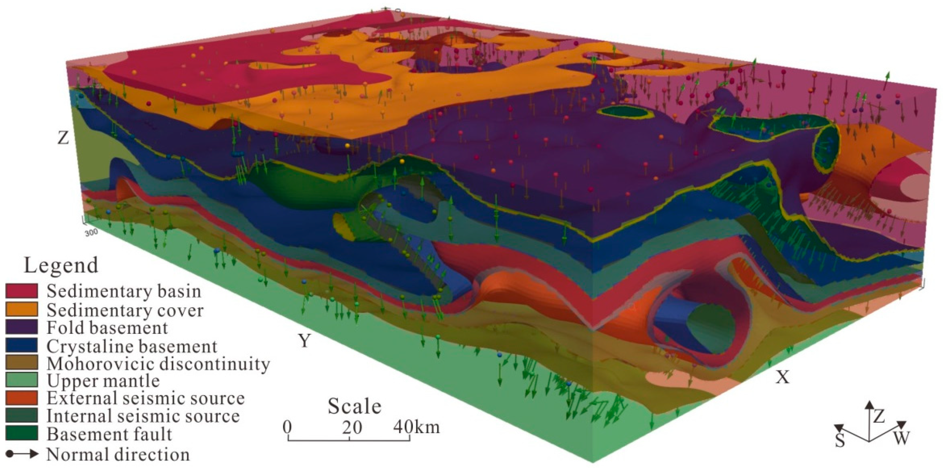
6. Crustal Medium Structure

In order to couple the above structural models into the prior comprehensive geological model, an appropriate modeling method was developed by integrating multi-source datasets such as topographic and geomorphic data, velocity structure dataset, fault plane data, seismic structure data, and Moho data. The topological relationship of crustal medium structure is established through the model calculation, the unified crustal medium structure model is finally generated, and the 3D format required for numerical simulation is derived, which can be used in the later finite element modeling. In addition, with the improvement of observation accuracy and the maturity of inversion methods, the result data used in modeling will be updated, and the corresponding model will be optimized accordingly, so that the model has a good inheritance. The model data can also be complex and diverse for the regions with different deep studies, making the model more adaptable.
By the modeling of crustal medium structure, the distribution characteristics of sedimentary cover, fold basement, and crystalline basement in the Xichang area are revealed (Figure 6). The complex fault plane cuts the base and forms the corresponding fracture zone. Because of its low mechanical strength, it is broken in the extrusion process and forms earthquakes. Moreover, there are low-velocity anomalies under Mt. Gongga with high terrestrial heat flow value, indicating that the region’s lithologic medium and physical state has changed significantly, resulting in the decline of its mechanical strength and a certain viscosity and ductility. There are also a lot of earthquakes around the lower part of Mt. Gongga, and the concentrated earthquake area further reveals the morphological characteristics of the focal region. The seismological velocity structure and fault model depend on and constrain each other and form the crustal medium structure model of the Xichang region together. Our model reveals better the relationship between different structures in the Xichang area, and the large-scale structure has good consistency with previous studies; the model provides more detailed features. It has obvious advantages in describing regional seismicity and can meet seismic scientific research and seismic engineering application modeling needs. Our model is significant for understanding the distribution and physical property differences of sub-blocks, structural characteristics and geodynamics problems, inversion, and other scientific problems.

7. Discussions and Conclusions

7.1. Discussion

There is complex structural morphology, crisscross of deep and large faults, and massive earthquakes in the Xichang area, which have produced rich seismic scientific research and structural models. Those results provide high-quality datasets for crustal medium structure modeling and are conducive to studying the automatic modeling technique. By means of automatic modeling, the results can well reflect the features of the regional crustal medium structure.
The crustal medium structure in the Xichang area shows that with the continuous enhancement of tectonic stress, the high-speed body is not easy to fracture due to its high degree of crystallization and strong mechanical properties of rock. Once it is fractured, the earthquake will focus on the fault section. However, the low-velocity body has potentially good ductility or rheology due to the participation of underground fluid or partial melting, which is mainly plastic deformation. The folded basement between the two is brittle and easy to release energy and cause earthquakes, and the penetration of the seismic fracture surface further forms a fault. It further explains why the fault plane is greatly affected by the shape of the high-speed body in the folded basement.
Combined with the fault morphology and source structure, it can be seen that the location of the earthquake in the study area is usually concentrated in three areas: (1) At the intersection of faults, the rocks in this area are broken. It is easy to be squeezed and deformed when the surrounding stress is strengthened, forming the mid-small events with high frequency and dense distribution. (2) The region with large fault bending amplitude, which is mainly influenced by the shape of a high-speed body, is prone to the locked status and stress concentration release and then forms a moderate earthquake. (3) The low-velocity zone, which is greatly affected by temperature and fluid, has certain rheological properties and ductility. The unloading area is formed around it, which can cause small and medium earthquakes. In summary, the crustal structure and geological mechanics background can control the stress distribution and energy release. Therefore, we can further calculate the stress distribution state and concentration area through numerical simulation and analyze the area where earthquakes may occur combined with the mechanical background of geological bodies. It can helpfully estimate the earthquake risk source and verify the reliability of the model based on the observation datasets.

7.2. Conclusions

Our main aim is to explore a new approach to automatically build a more realistic crustal medium structure model based on the previous results, which can be used in the later geophysical field simulation and forecast. It is a comprehensive application of previous research results, and its main data sources rely on velocity structure data, geological structure data, and relocated earthquake catalog. Therefore, modeling uncertainty is also limited by the used prior research results. With further research, the accuracy of various input data may be improved, and the crustal medium structure model will be continuously updated to reflect the real seismogenic structure.
Moreover, the efficient automatic modeling technique can more efficiently make the conversion from the numerous geoscience datasets to the comprehensive model, which can not only be used for mutual verification of the reliability of research results, but also better serve the earthquake engineering, earthquake emergency response, and operational earthquake prediction.
Finally, we need to select the model scale and to combine this with the actual scenario. In this case of the Xichang crustal medium we show clearly that the accuracy of the kilometer level is able to satisfy the description of the structural characteristics of large-scale seismotectonic units. If there is a higher precision model scenario, it may bring higher data redundancy and increase the burden of model calculation. Therefore, the accuracy of datasets and modeling purpose is mutually dependent. The reasonable trade-off can provide a good balance between the modeling difficulty and scenario application.

Author Contributions

Conceptualization, H.Z. and S.C.; methodology, L.-W.G., and S.C.; software, S.C.; validation, S.C., and L.-J.C.; formal analysis, S.C., and L.-J.C.; investigation, L.-J.C.; resources, S.C.; data curation, L.-J.C.; writing—original draft preparation, L.-W.G.; writing—review and editing, H.Z. and S.C.; visualization, L.-W.G.; supervision, H.Z.; project administration, S.C.; funding acquisition, S.C. and H.Z. All authors have read and agreed to the published version of the manuscript.

Funding

National Natural Science Foundation of China (U1939205) and the National Key R&D Program of China (2017YFC1500503).

Informed Consent Statement

Not applicable.

Data Availability Statement

Initial fault data and precise location data provided by the China Earthquake Scientific Experimental Site (http://www.cses.ac.cn, accessed on 30 January 2022), and velocity structure model data from China Geophysical Reference Model (http://chinageorefmodel.org, accessed on 30 January 2022).

Acknowledgments

We acknowledge the initial fault data and precise location data provided by the China Earthquake Scientific Experimental Site (http://www.cses.ac.cn, accessed on 30 January 2022). I am also grateful to Fang Lihua for providing earthquake catalog and Wan Yongge for providing the focal mechanism solution results and David A. Yuen from Columbia University and Gabriele Morra from University of Lousiana for constructive suggestions and comments.

Conflicts of Interest

The authors declare no conflict of interest.

References

  1. Yao, H. Building the community velocity model in the Sichuan-Yunnan region, China: Strategies and progresses. Sci. China Earth Sci. 2020, 63, 1425–1428. [Google Scholar] [CrossRef]
  2. Jiang, C.S.; Fang, L.H.; Han, L.B.; Wang, W.L.; Guo, L.J. Assessment of earthquake detection capability for the seismic array: A case study of the Xichang seismic array. Chin. J. Geophys. 2015, 58, 832–843. (In Chinese) [Google Scholar]
  3. He, H.-L.; Yasutakyr, I. Faulting on The Anninghe Fault Zone, Southwest China in Late Quaternary and Its Movement Model. Acta Seismol. Sinica 2017, 29, 537–548. (In Chinese) [Google Scholar] [CrossRef]
  4. Lu, R.Q. The fault model in China Seismic Experimental Site. In China Seismic Experimental Site; Springer: Singapore, 2019. [Google Scholar] [CrossRef]
  5. Lu, R.Q.; Liu, Y.D.; Xu, X.W.; Tan, X.B.; He, D.F.; Yu, G.H.; Cai, M.G.; Wu, X.Y. Three-Dimensional Model of the Lithospheric Structure Under the Eastern Tibetan Plateau: Implications for the Active Tectonics Seismic Hazards. Tectonics 2019, 38, 1292–1307. [Google Scholar] [CrossRef]
  6. Yi, G.X.; Long, F.; Zhao, M.; Gong, Y.; Qiao, H.Z. Focal Mechanism and Seismogenic Structure of The M5.0 Yuexi Earthquake On 1 Oct. 2014, South Western China. Seismol. Geol. 2016, 38, 1124–1136. (In Chinese) [Google Scholar]
  7. Li, J.; Wang, Q.C.; Cui, Z.J.; Zhang, P.; Zhou, L.; Zhou, H. Characteristics of Focal Mechanisms and Stress Field in the Eastern Boundary of Sichuan-Yunnan Block and Its Adjacent Area. Seismol. Geol. 2019, 41, 1395–1412. (In Chinese) [Google Scholar]
  8. Zhou, L.Q.; Xia, J.Y.; Shen, W.S.; Zheng, Y.; Yang, Y.J.; Shi, H.X.; Ritzwoller, M.H. The structure of the crust and uppermost mantle beneath South China from ambient noise and earthquake tomography. Geophys. J. Int. 2012, 189, 1565–1583. [Google Scholar]
  9. Yang, Y.; Ritzwoller, M.H.; Zheng, Y.; Shen, W.S.; Levshin, A.L.; Xie, Z.J. A synoptic view of the distribution and connectivity of the mid-crustal low velocity zone beneath Tibet. J. Geophys. Res. 2012, 117, B04303. [Google Scholar] [CrossRef]
  10. Zhao, L.F.; Xie, X.B.; He, J.K.; Tian, X.; Yao, Z.X. Crustal flow pattern beneath the Tibetan Plateau constrained by regional Lg-wave Q tomography. Earth Planet Sci. Lett. 2013, 383, 113–122. [Google Scholar] [CrossRef]
  11. Wei, W.; Zhao, D.; Xu, J.; Zhou, B.; Shi, Y. Depth variations of P-wave azimuthal anisotropy beneath Mainland China. Sci. Rep. 2016, 6, 29614. [Google Scholar] [CrossRef] [Green Version]
  12. Shen, W.; Ritzwoller, M.H.; Kang, D.; Kim, Y.H.; Lin, F.C.; Ning, J.; Wang, W.; Zheng, Y.; Zhou, L. A seismic reference model for the crust and uppermost mantle beneath China from surface wave dispersion. Geophys. J. Int. 2016, 206, 954–979. [Google Scholar] [CrossRef] [Green Version]
  13. Tan, X.L.; Fang, L.H.; Wang, W.L.; Wu, J.P. Rayleigh Wave Group Velocity Tomography with Ambient Noise in the Anninghe-Zemuhe FaultZone and Its Surrounding Areas. Earthq. Res. China 2018, 34, 400–413. (In Chinese) [Google Scholar]
  14. Xin, H.; Zhang, H.; Kang, M.; He, R.; Gao, L.; Gao, J. High resolution lithospheric velocity structure of continental China by double-difference seismic travel-time tomography. Seismol. Res. Lett. 2019, 90, 229–241. [Google Scholar] [CrossRef]
  15. Liu, Y.; Yao, H.J.; Zhang, H.H.; Fang, H. The Community Velocity Model, V.1.0 of Southwest China, Constructed from Joint Body- and Surface-Wave Travel-Time Tomography. Seismol. Res. Lett. 2021, 92, 2972–2987. [Google Scholar] [CrossRef]
  16. Han, S.; Zhang, H.; Xin, H.; Shen, W.; Yao, H. USTClitho2.0: Updated Unified Seismic Tomography Models for Continental China Lithosphere from Joint Inversion of Body-Wave Arrival Times and Surface Wave Dispersion Data. Seismol. Res. Lett. 2022, 93, 201–215. [Google Scholar] [CrossRef]
  17. Shang, Y.J.; Yang, C.G.; Jin, W.J.; Chen, Y.W.; Hasan, M.; Wang, Y.; Li, K.; Lin, D.M.; Zhou, M. Application of Integrated Geophysical Methods for Site Suitability of Research Infrastructures (RIs) in China. Appl. Sci. 2021, 11, 8666. [Google Scholar] [CrossRef]
  18. Zhang, Z.; Zhang, H.; Wang, L.S.; Cheng, H.H.; Shi, Y.L. Late Cenozoic structural deformation and evolution of the central-southern Longmen Shan fold-and-thrust belt, China: Insights from numerical simulations. J. Asian Earth Sci. 2019, 176, 88–104. [Google Scholar] [CrossRef]
  19. Zhang, H.; Wu, Z.L.; Zhang, D.L.; Liu, J.; Wang, H.; Yan, Z.Z.; Shi, Y.L. Virtual Sichuan-Yunnan—Design and construction of regional strong earthquake evolution numerical model based on ten million mesh parallel finite element calculation. Sci. China Earth Sci. 2009, 39, 260. [Google Scholar] [CrossRef]
  20. Kong, Q.; Trugman, D.T.; Ross, Z.E.; Bianco, M.J.; Meade, B.J.; Gerstoft, P. Machine Learning in Seismology: Turning Data into Insights. Seismol. Res. Lett. 2019, 90, 3–14. [Google Scholar] [CrossRef] [Green Version]
  21. Bergen, K.J.; Johnson, P.A.; Maarten, V.; Beroza, G.C. Machine learning for data-driven discovery in solid Earth geoscience. Science 2019, 363, eaau0323. [Google Scholar] [CrossRef]
  22. Joshi, A.; Kaur, R. A review: Comparative study of various clustering techniques in data mining. Int. Adv. Res. Comp. Sci. Softw. Eng. 2015, 1, 1–4. [Google Scholar]
  23. Trugman, D.T.; Shearer, P.M. GrowClust: A hierarchical clustering algorithm for relative earthquake relocation, with application to the Spanish Springs and Sheldon, Nevada, earthquake sequences. Seismol. Res. Lett. 2017, 88, 379–391. [Google Scholar] [CrossRef]
  24. Kuang, W.; Yuan, C.; Zhang, J. Real-time determination of earthquake focal mechanism via deep learning. Nat. Commun. 2021, 12, 1432. [Google Scholar] [CrossRef]
  25. Yin, J.; Li, Z.; Denolle, M. Source time function clustering reveals patterns in earthquake dynamics. Seismol. Res. Lett. 2021, 92, 2343–2353. [Google Scholar] [CrossRef]
  26. Ansari, A.; Firuzi, E.; Etemadsaeed, L. Delineation of Seismic Sources in Probabilistic Seismic-Hazard Analysis Using Fuzzy Cluster Analysis and Monte Carlo Simulation. Bull. Seismol. Soc. Am. 2015, 105, 2174–2191. [Google Scholar] [CrossRef]
  27. Ester, M.; Kriegel, H.P.; Sander, J.; Xu, X. A density-based algorithm for discovering clusters in large spatial databases with noise. In Proceedings of the Second International Conference on Knowledge and Data Mining, AAAI Press 96, Portland, OR, USA, 2–4 August 1996; pp. 226–231. [Google Scholar]
  28. Ouillon, G.; Sornette, D. Segmentation of fault networks determined from spatial clustering of earthquakes. J. Geophys. Res. Solid Earth 2011, 116, B02306. [Google Scholar] [CrossRef] [Green Version]
  29. Wang, Y.; Ouillon, G.; Woessner, J.; Sornette, D.; Husen, S. Automatic reconstruction of fault networks from seismicity catalogs including location uncertainty. J. Geophys. Res. Solid Earth 2013, 118, 5956–5975. [Google Scholar] [CrossRef] [Green Version]
  30. Kaven, J.O.; Pollard, D.D. Geometry of crustal faults: Identification from seismicity and implications for slip and stress transfer models. J. Geophys. Res. Solid Earth 2013, 118, 5058–5070. [Google Scholar] [CrossRef]
  31. Brunsvik, B.; Morra, G.; Cambiotti, G.; Yuen, D.A. Three-dimensional paganica fault morphology obtained from hypocenter clustering (L’Aquila 2009 seismic sequence, Central Italy). Tectonophysics 2021, 804, 228756. [Google Scholar] [CrossRef]
  32. Cong, B.L.; Zhao, D.S.; Zhang, W.H.; Zhang, Z.Z.; Yang, M. Characteristics of Magmatic Activity in the Sichang Area and Its Bearing on the Tectonic Geological Development. Sci. Geol. Sin. 1973, 8, 175–195. (In Chinese) [Google Scholar]
  33. Liu, F.H. Characteristics of geological structure and seismicity in Xichang area. J. Chengdu Inst. Geol. 1982, 23–28. (In Chinese) [Google Scholar]
  34. He, H.L.; Ikeda, Y.; He, Y.L.; Togo, M.; Chen, J.; Chen, C.; Tajikara, M.; Echigo, T.; Okada, S. Newly-generated Daliangshan Fault zone-Shortcutting on the central section of Xianshuihe-Xiaojiang Fault system. Sci. China Ser. D Earth Sci. 2008, 51, 1248–1258. [Google Scholar] [CrossRef]
  35. Wen, X.Z. Character of rupture segmentation of the Xianshuihe-Anninghe-Zemuhe fault zone, western Sichuan. Seismol. Geol. 2000, 22, 239–249. [Google Scholar]
  36. Cheng, J.; Liu, J.; Xu, X.W.; Gan, W.J. Tectonic Characteristics of Strong Earthquakes in Daliangshan Sub-Block and Impact of the MS6.5 Ludian Earthquake in 2014 on the Surrounding Faults. Seismol. Geol. 2014, 36, 1228–1243. (In Chinese) [Google Scholar]
  37. Hu, Y.X.; Zeng, Z.; Li, C.J.; Li, Y.H.; Song, S.W. Research on Present-day Crustal Deformation and Fault Activities in Xichang Area. Earthquake 2020, 40, 62–72. (In Chinese) [Google Scholar]
  38. Sun, H.Y.; He, H.L.; Wei, Z.Y.; Gao, W. Late Quaternary Activity of Zhuma Fault on the North Segment of Daliangshan Fault Zone. Seismol. Geol. 2015, 37, 440–454. (In Chinese) [Google Scholar]
  39. Wei, Z.Y.; He, H.L.; Shi, F.; Xu, Y.R.; Sun, H.Y. Slip Rate on the South Segment of Daliangshan Fault Zone. Seismol. Geol. 2012, 34, 282–293. (In Chinese) [Google Scholar]
  40. He, M.X.; Fang, H.; Wang, X.B.; Jing-Qi, L.U.; Yuan, Y.Z.; Bai, D.W.; Bing-Rui, D.U.; Qiu, G.G.; Gao, B.T. Deep Conductivity Characteristics of The Southern Xianshuihe Fault Zone. Chin. J. Geophys. 2017, 60, 2414–2424. (In Chinese) [Google Scholar] [CrossRef]
  41. Li, D.H.; Ding, Z.F.; Wu, P.P.; Liang, M.; Gu, Q.P. Deep structure of the Zhaotong and Lianfeng fault zones in the eastern segment of the Sichuan-Yunnan border and the 2014 Ludian MS6.5 earthquake. Chin. J. Geophys. 2019, 62, 4571–4587. (In Chinese) [Google Scholar] [CrossRef]
  42. Si, Z.Y.; Jiang, C.S. Research on Parameter Calculation for the Ogata–Katsura 1993 Model in Terms of the Frequency–Magnitude Distribution Based on a Data-Driven Approach. Seismol. Res. Lett. 2019, 90, 1318–1329. [Google Scholar] [CrossRef]
  43. Grada, M.; Polkowskia, M.; Ostaficzukb, S.R. High-resolution 3D seismic model of the crustal and uppermost mantle structure in Poland. Tectonophysics 2016, 666, 188–210. [Google Scholar] [CrossRef]
  44. Moschetti, M.P.; Ritzwoller, M.H.; Lin, F.C. Seismic evidence for widespread crustal deformation caused by extension in the western USA. Nature 2010, 464, 885–889. [Google Scholar] [CrossRef]
  45. Mos5chetti, M.P.; Ritzwoller, M.H.; Lin, F.C.; Yang, Y. Crustal shear velocity structure of the western US inferred from amient noise and earthquake data. Geophys. Res. 2010, 115, B007448. [Google Scholar] [CrossRef]
  46. Manu-Marfo, D.; Aoudia, A.; Pachhai, S.; Kherchouche, R. 3D shear wave velocity model of the crust and uppermost mantle beneath the Tyrrhenian basin and margins. Sci. Rep. 2019, 9, 3609. [Google Scholar] [CrossRef]
  47. Qiu, Q.; Hill, E.M.; Barbot, S.; Hubbard, J.; Feng, W.; Lindsey, E.O.; Tapponnier, P. The mechanism of partial rupture of a locked megathrust: The role of fault morphology. Geology 2016, 44, 875–878. [Google Scholar] [CrossRef]
  48. Lohr, T.; Krawczyk, C.M.; Oncken, O.; Tanner, D.C. Evolution of a fault surface from 3D attribute analysis and displacement measurements. J. Struct. Geol. 2008, 30, 690–700. [Google Scholar] [CrossRef] [Green Version]
  49. Røe, P.; Georgsen, F.; Abrahamsen, P. An uncertainty model for fault shape and location. Math. Geosci. 2014, 46, 957–969. [Google Scholar] [CrossRef] [Green Version]
Figure 1. Seismicity and seismotectonic setting in the study area.
Applsci 12 02955 g001
Figure 2. Workflow of modeling.
Applsci 12 02955 g002
Figure 3. Velocity profile and structural characteristics. Velocity profile characteristics in each direction after interpolation (a), crustal medium layer based on profile feature extraction (b), interpret crustal medium structure by combining geological structure and seismic data (c).
Applsci 12 02955 g003
Figure 4. Results of seismic clustering analysis and extraction of fault morphological features. Classification of earthquakes by faults based on supervised classification (a), earthquakes associated with faults were obtained based on cluster analysis (b), morphological features of fault plane were extracted based on spline interpolation (c).
Applsci 12 02955 g004
Figure 5. Feature extraction of seismotectonic structure. The optimal clustering parameters were obtained by evaluating different cluster parameters based on the Silhouette Coefficient (a), analyzing results based on DBSCAN (ε = 0.58, MinPts = 70) (b), results of equivalent seismic particle analysis, and kernel density calculation (c), seismotectonic structure extraction based on seismic kernel density isosurface (d).
Applsci 12 02955 g005
Figure 6. Modeling results of crustal medium structure.
Applsci 12 02955 g006
Table 1. Comparison of seismological velocity models.
Regional ModelInversion MethodH ResolutionV ResolutionDataset
USTClitho2.0Joint Inversion0.5°5 kmHan et al., 2021 [16]
SWChinaCVM-1.0Joint Inversion0.5°5 kmLiu et al., 2021 [15]
USTClitho1.0DD seismic tomography0.5° × 0.5°5 kmXin et al., 2019 [14]
Xichang RegionAmbient noise tomography20–40 km20 kmTan et al., 2018 [13]
ChinaSurface wave dispersion0.5° × 0.5°0.5 kmShen et al., 2016 [12]
Mainland ChinaP-wave anisotropic tomography0.7° × 0.7°35 kmWei et al., 2016 [11]
Tibetan PlateauLg-wave Q tomography1° × 1°0.2 kmZhao et al., 2013 [10]
TibetAmbient noise tomography1° × 1°0.2 kmYang et al., 2012 [9]
South ChinaAmbient noise tomography0.5° × 0.5°0.2 kmZhou et al., 2012 [8]
H&V resolution: Refers to the horizontal or vertical resolution of data supported by shared data.
Table 2. Initial parameters of the fault model.
FaultsLength (km)StrikeDipDip AngleFault PropertyData Sources
Xianshuihe Fault (Moxi)600340°70°85°Strike-slipChen et al., 2014 [36]
Longmenshan Fault600273°80°ThrustLu, 2019 [5]
Xiaojinhe Fault30045°315°70°Strike-slipChen et al., 2014 [36]
Qinhe Fault200275°70°Strike-slipLu, 2019 [4]
Mopanshan Fault300178°268°83°Strike-slipLu, 2019 [4]
Anninghe Fault300173°83°80°Strike-slipHe et al., 2007 [34]
Zemuhe Fault300330°45°70°Strike-slipChen et al., 2014 [36]
Daliangshan Fault (N)300160°250°55°Strike-slipChen et al., 2014 [36]
Daliangshan Fault (S)300180°270°55°Strike-slipSun et al., 2016 [38]
Table 3. Focal mechanism solutions.
Longitude (°)Latitude (°)Depth (km)MagPlane 1Plane 2Fault
s1d1r1s2d2r2
102.4527.57−5417974−299862−162ZMHF
102.4927.44−34.21579006790−180ZMHF
101.829.6−285.6059108581149LMSF
101.929.4−256.5965−1710675−154LMSF
102.8427.88−73.617279138077169DLSF
102.7827.98−194.61728038187170DLSF
102.7927.98−84.717275−78383−164DLSF
102.7928.4−9.35.116980247466169DLSF
102.7328.37−155.617082317559171DLSF
102.7928.4−95.116980257466169DLSF
102.81528.32−143.214861−116380−150DLSF
102.2729.18−64.41737808390168DLSF
102.2829.15−144.858129588171ANHF
102.2529.01−1041079−610184−168ANHF
102.3629.06−263.688217399848ANHF
102.2529.09−54.216686175735238XSHF
102.2729.18−64.41737808390168XSHF
Publisher’s Note: MDPI stays neutral with regard to jurisdictional claims in published maps and institutional affiliations.

