A Fuzzy Logic Reinforcement Learning Control with Spring-Damper Device for Space Robot Capturing Satellite

Abstract

In order to prevent joints from being damaged by impact force in a space robot capturing satellite, a spring-damper device (SDD) is added between the joint motor and manipulator. The device can not only absorb and attrition impact energy, but also limit impact force to a safe range through reasonable design compliance control strategy. Firstly, the dynamic mode of the space robot and target satellite systems before capture are established by using a Lagrange function based on dissipation theory and Newton-Euler function, respectively. After that, the impact effect is analyzed and the hybrid system dynamic equation is obtained by combining Newton’s third law, momentum conservation, and a kinematic geometric relationship. To realize the buffer compliance stability control of the hybrid system, a reinforcement learning (RL) control strategy based on a fuzzy wavelet network is proposed. The controller consists of a performance measurement unit (PMU), an associative search network (ASN), and an adaptive critic network (ACN). Finally, the stability of system is proved by Lyapunov theorem, and both the impact resistance of SDD and the effectiveness of buffer compliance control strategy are verified by numerical simulation.

1. Introduction

Space exploration is of great significance to the development of resources exploration, meteorological observation, navigation, and positioning, so a large number of satellites are launched into space every year. It is inevitable that a small part of satellites will fail to enter the intended orbit or damage in orbit. If the satellites can be recovered, the cost of space exploration will be greatly saved. At present, it is feasible to use a space robot to complete the capture task. This has therefore become one of the research hot spots of space exploration [1,2,3,4,5,6,7,8]. Generally, the process of capture operation can be divided into four stages: (1) the space robot observes the target satellite; (2) a pre-operation stage before capture operation, such as deceleration and detumbling control of the target satellite; (3) contact and collision between the space robot and target satellite; and (4) the stabilization control of the closed chain hybrid system. The impact force makes it easy to damage the joints of space robot in the third stage, and the impact effect will make the hybrid system unstable in the fourth stage. Therefore, these two stages represent the focus and challenges of this study.

For the third stage, Cheng et al. [9] analyzed the dynamic evolution for dual-arm space robot with capturing a spin satellite and calm control for unstable closed chain composite system are discussed. Uyama et al. [10] presented the impedance-based contact control of a free-flying space robot utilizing a compliant wrist for non-cooperative satellite capture operation. An open loop impedance control law based on contact dynamics model is introduced to realize the desired coefficient of restitution defined between the manipulator hand of a space robot and a contact point on a free-flying target. Dimitrov et al. [11] established the contact dynamic model of a space robot capturing satellite and analyzed the momentum exchange problem in the capture process. Yoshida et al. [12] studied the collision dynamics and kinematics of a space robot capturing satellite based on momentum conservation. Dong et al. [13] approximately described the elastic deformation of flexible manipulator by using the assumed mode method, and then analyzed the collision dynamics of space robot capturing satellite by combining the momentum impulse. It is worth noting that scholars mainly focus on the analysis of collision dynamics, and they do not pay attention to the protection of the joints. In fact, if the joints are not protected during the capture operation, they will be damaged by impact force and could even cause damage to the space robot.

A series elastic actuator (SEA) is usually added between the joint motor and manipulator in the ground robot, which can avoid joint being damaged by impact force when the robot collides with the external environment [14,15,16,17,18,19,20,21]. However, the space robot is a rootless system, and it works in both microgravity and a vacuum. If the SEA is added in the joints of space robot (refer to our published previously work [3,22]), the flexible vibration caused by SEA will be difficult to suppress. Therefore, the controller was divided into a fast subsystem controller and slow subsystem controller, wherein the slow subsystem controller realizes trajectory tracking and the fast subsystem controller suppresses the flexible vibration. This means that the controller becomes more complex, and the joint motor needs to provide additional torque to suppress flexible vibration. Sometimes this torque will exceed the load capacity of the motor. In order to cope with the problem, this paper adds a spring-damper device (SDD) between the joint motor and manipulator. Compared with SEA, The SDD can not only absorb and digest the impact energy, but also quickly attenuate the flexible vibration to achieve the suppression of flexible vibration.

For the fourth stage, Liu et al. [23] used impedance control to stabilize the hybrid system after space robot captures satellite. Huang et al. [24] designed a reconfigurable control system for attitude takeover control of target spacecraft, which considers the changes of mass properties and reaction wheels’ configuration. Luo et al. [25] proposed a robust inertia free attitude takeover control scheme with guaranteed prescribed performance for post capture combined spacecraft with consideration of unmeasurable states, unknown inertial property, and external disturbance torque. Gangapersaud et al. [26] presented a novel detumbling strategy for realizing detumbling of a non-cooperative, tumbling target by a space robot without prior knowledge of the target’s inertial parameters (mass, inertia tensor, location of center of mass). However, the impact effect is not considered in the above control schemes. When the impact effect exceeds a certain value, the hybrid system will lose stability, which makes it difficult to realize stability control.

In recent years, intelligent algorithms have been more and more applied to the control of robot systems [27,28,29]. Since the target satellite has a large initial velocity, the hybrid system after capture will be in a serious unstable state (e.g., involving overturning and rotation) and the traditional control method will make it difficult to complete its calm control. The actor-critic reinforcement learning (RL) control can optimize itself through trial-and-error and interaction with dynamic environment, and has strong environmental adaptability [30,31,32,33,34]. Therefore, an RL control scheme based on fuzzy wavelet network is proposed to realize stabilization of the hybrid system. The controller consists of a performance measurement unit (PMU), an associative search network (ASN) and an adaptive critic network (ACN). The controller obtains the primary reinforcement signal through the PMU, and then uses the ACN to collect the primary reinforcement signal for generating the enhancement signal, which is used to adjust the ASN dominate strategy function to realize the hybrid system stability control. The mechanism of the proposed reinforcement learning can be found in [35]. The food is the primary reinforcement signal, and the bell is the secondary reinforcement signal. In order to maintain a stronger effect, the food and the bell are matched to generate the enhancement signal. Compared to RL in our published previously work [3], this paper enhanced the primary reinforcement signal to become an enhancement signal containing more information (which ultimately makes the calm control of the hybrid system more stable).

This paper is organized as follows. In Section 2, the structure of the SDD and the buffer compliance strategy are described. In Section 3, the hybrid system dynamic model is obtained, and the impact effect and force are analyzed. Furthermore, a RL control strategy based on fuzzy wavelet network is designed in Section 4. The results of the simulation are given in Section 5. Finally, the conclusion is summarized in Section 6.

2. Structure of the SDD and Buffer Compliance Strategy

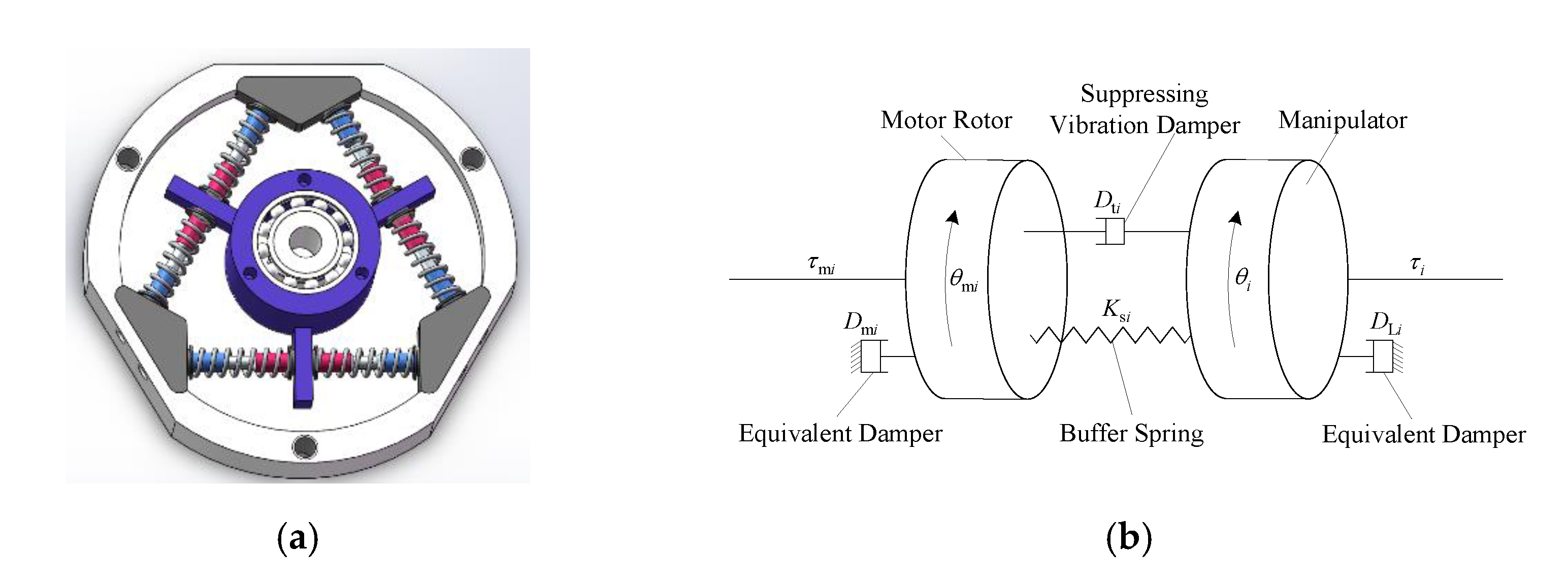
2.1. Structure of the SDD

Compared with our published previously work [3], dampers are added. The structure diagram of the SDD is shown in Figure 1. The spring is used to absorb impact energy, and the damper provides damping force in real time to suppress flexible vibration. In order to describe the resistance of motor and manipulator more realistically, the equivalent dampers are added to them, respectively (in fact, there are no dampers), and the connection mode of the SDD is shown in Figure 2. In Figure 1, $K_{\mathrm{s}i}, D_{ti}(i=1,2,\cdot \cdot \cdot ,n)$ are the stiffness of torsion spring and the damping coefficient of rotary damper, $D_{mi}, D_{Li}(i=1,2,\cdot \cdot \cdot ,n)$ are the damping coefficient of equivalent damper at motor and manipulator.

2.2. Buffer Compliance Strategy

In the third stage, the end-effector of space robot collides with the target satellite, and the impact energy will be quickly buffered and consumed by SDD when it is transmitted to the motor rotors so as to protect the joints. In the fourth stage, due to the impact effect, the instantaneous impact torque will be generated when the motors are turned on. If the instantaneous impact torque exceeds the limit of joint and the motor still turns on, the joint will be damaged. Therefore, it is necessary to set a torque threshold according to the ultimate torque value that the joints can withstand. When the instantaneous impact torque is detected to exceed the set threshold, the motor will be turned off. At this time, the spring will provide elasticity to mitigate the impact torque on joints, and the damper will quickly dissipate energy to suppress the flexible vibration. However, if only set one threshold is turned on, the motors will be frequently switched (which easily causes motor damage). The buffer compliance strategy proposed in this paper set a threshold in order to turn on and off at the same time. When the impact torques of the joints exceed the turn off torque threshold, the motor is turned off; when the impact torque is reduced to the turn on threshold by SDD, the motor is turned on again.

3. Dynamic Modeling and Impact Analysis

The structure of a space robot with SDD and target satellite systems is shown in Figure 3. The $O_0$, $O_{\mathrm{s}}$ and $O_i(i=1,2,\cdot \cdot \cdot ,n)$ are the centroids of carrier, satellite, and joints respectively. P and P′ are the acquisition point of space manipulator and the acquisition point of satellite, respectively. $xOy$ is the inertial coordinate system moving with orbit, $x_0{O}_0{y}_0$ and $x_{\mathrm{s}}{O}_{\mathrm{s}}{y}_{\mathrm{s}}$ are the coordinate systems fixed on the centroids of carrier and satellite, respectively, $x_i{O}_i{y}_i(i=1,2,\cdot \cdot \cdot ,n)$ is the coordinate system fixed at the centre of ith joint. The parameters of space robot and satellite are defined as follows: $m_0$, $m_i(i=1,2,\cdot \cdot \cdot ,n)$ and $m_{\mathrm{s}}$ are the mass of space robot carrier, manipulator, and satellite, respectively, $I_i$, $I_{mi}(i=1,2,\cdot \cdot \cdot ,n)$ and $I_{\mathrm{s}}$ are the moment of inertia of manipulator, motor rotor and satellite respectively, $d_0$, $d_i(i=1,2,\cdot \cdot \cdot ,n)$ and $d_{\mathrm{s}}$ are the distance from $O_0$ to $O_1$, from the centre of joint to manipulator and from satellite centroid to the end, respectively. $L_i(i=1,2,\cdot \cdot \cdot ,n)$ is the length of the manipulator, and ${\theta }_0$, ${\theta }_i$, ${\theta }_{\mathrm{s}}$, and ${\theta }_{mi}(i=1,2,\cdot \cdot \cdot ,n)$ are the angle of carrier attitude, manipulator, satellite attitude, and motor rotor, respectively.

As the system of space robot with SDD (see Figure 3), the total kinetic energy of space robot in the pre-contact phase is as follows:

$$T_{\mathrm{r}}=\frac{1}{2}{\displaystyle \sum _{i=0}^n\left(m_i{\dot{r}}_i^{\mathrm{T}}{\dot{r}}_i+I_i{\omega }_i^2\right)}+\frac{1}{2}{\displaystyle \sum _{j=1}^n\left(I_{mj}{\omega }_{mj}^2\right)}$$

(1)

where $r_i$ is the position vector of manipulator’s mass centre, and ${\omega }_i$ and ${\omega }_{mj}$ are the angular velocity of manipulator and motor rotor, respectively.

If the microgravity is ignored, the potential energy of space robot comes from the spring in SDD:

$$U_{\mathrm{r}}=\frac{1}{2}{\displaystyle \sum _{i=1}^n\left[k_{\mathrm{s}i}{({\theta }_{mi}-{\theta }_i)}^2\right]}$$

(2)

Due to the addition of SDD in the joints of space robot, the space robot is a nonpotential system, the dissipation function should be added:

$${\vartheta }_{\mathrm{r}}={\displaystyle \sum _{i=1}^n\left[D_{mi}{\dot{\theta }}_{mi}^2+D_{ti}{({\dot{\theta }}_{mi}-{\dot{\theta }}_i)}^2+D_{Li}{\dot{\theta }}_i^2\right]}$$

(3)

Reference [36], the Lagrange equation of dissipative system is as follows:

$$\frac{d}{dt}\left(\frac{\partial L_{\mathrm{r}}}{\partial {\dot{\mathit{q}}}_{\mathrm{r}}}\right)-\frac{\partial L_{\mathrm{r}}}{\partial {\mathit{q}}_{\mathrm{r}}}+\frac{\partial {\vartheta }_{\mathrm{r}}}{\partial {\dot{\mathit{q}}}_{\mathrm{r}}}=\mathit{Q}$$

(4)

Combined Equations (1)–(4), the model of space robot system before capture is obtained as follows:

$$\left\{\begin{array}{l}{M}_{\mathrm{r}}(q_{\mathrm{r}}){\ddot{\mathit{q}}}_{\mathrm{r}}+\left(H_{\mathrm{r}}(q_{\mathrm{r}},{\dot{\mathit{q}}}_{\mathrm{r}})+D_{\mathrm{L}}\right){\dot{\mathit{q}}}_{\mathrm{r}}={\tau }_{\mathrm{r}}+J_{\mathrm{r}}^{\mathrm{T}}{F}_{\mathrm{P}}\\ I_{\mathrm{m}}{\ddot{\mathit{q}}}_{\mathrm{m}}+D_{\mathrm{mc}}{\dot{\mathit{q}}}_{\mathrm{m}}+{\tau }_{\mathrm{c}}={\tau }_{\mathrm{m}}\\ K_{\mathrm{s}}(q_{\mathrm{m}}-q_{\mathrm{c}})+D_{\mathrm{tc}}({\dot{\mathit{q}}}_{\mathrm{m}}-{\dot{\mathit{q}}}_{\mathrm{c}})={\tau }_{\mathrm{c}}\end{array}\right.$$

(5)

where $M_{\mathrm{r}}\in R^{(n+3)\times (n+3)}$ is the symmetric positive definite inertia matrix of space robot, $H_{\mathrm{r}}\in R^{(n+3)\times (n+3)}$ is the matrix containing Coriolis force and centrifugal force, $D_{\mathrm{L}}\in R^{(n+3)\times (n+3)}$ is the augmented equivalent damper coefficient matrix of manipulator, $D_{\mathrm{mc}}\in R^{n\times n}$ is the equivalent damper coefficient matrix of motor, $D_{\mathrm{tc}}\in R^{n\times n}$ is the damper coefficient matrix in SDD. $q_{\mathrm{r}}={[x_0,y_0,{\theta }_0,q_{\mathrm{c}}^{\mathrm{T}}]}^{\mathrm{T}}$ is the generalized coordinate of space robot system, and $q_{\mathrm{c}}={[{\theta }_1,{\theta }_2,\cdot \cdot \cdot ,{\theta }_n]}^{\mathrm{T}}$, $q_{\mathrm{m}}={[{\theta }_{\mathrm{m}1},{\theta }_{\mathrm{m}2},\cdot \cdot \cdot ,{\theta }_{\mathrm{m}n}]}^{\mathrm{T}}$. ${\tau }_{\mathrm{r}}={[{\tau }_{\mathrm{B}}^{\mathrm{T}},{\mathit{\tau }}_0,{\tau }_{\mathrm{c}}^{\mathrm{T}}]}^{\mathrm{T}}$, ${\tau }_{\mathrm{B}}={[0,0]}^{\mathrm{T}}$, ${\tau }_0$ is the input torque of carrier, ${\tau }_{\mathrm{c}}={[{\tau }_1,{\tau }_2,\cdot \cdot \cdot ,{\tau }_n]}^{\mathrm{T}}$ is the joint input torque, ${\tau }_{\mathrm{mc}}={[{\tau }_{\mathrm{m}1},{\tau }_{\mathrm{m}2},\cdot \cdot \cdot ,{\tau }_{\mathrm{m}n}]}^{\mathrm{T}}$ is the motor output torque.$I_{\mathrm{m}}={[I_{\mathrm{m}1},I_{\mathrm{m}2},\cdot \cdot \cdot ,I_{\mathrm{m}n}]}^{\mathrm{T}}$ is the inertia matrix of motor rotor, $K_{\mathrm{s}}={[k_{\mathrm{s}1},k_{\mathrm{s}2},\cdot \cdot \cdot ,k_{\mathrm{s}n}]}^{\mathrm{T}}$ is the stiffness matrix of spring. $J_{\mathrm{r}}\in R^{3\times (n+3)}$ is the Jacobian matrix of space robot, $F_{\mathrm{P}}\in R^{3\times 1}$ is the force acting on the end-effector of space robot.

The model of satellite system before capture is obtained by the Newton–Euler equation:

$$M_{\mathrm{s}}{\ddot{\mathit{q}}}_{\mathrm{s}}=J_{\mathrm{s}}^{\mathrm{T}}{F}_{{\mathrm{p}}^{\prime }}$$

(6)

where $M_{\mathrm{s}}\in R^{3\times 3}$ is the symmetric positive definite inertia matrix of satellite, $q_{\mathrm{s}}={[x_{\mathrm{s}},y_{\mathrm{s}},{\theta }_{\mathrm{s}}]}^{\mathrm{T}}$ is the generalized coordinate of satellite system, $x_{\mathrm{s}}$ and $y_{\mathrm{s}}$ are the satellite centroid coordinates, $J_{\mathrm{s}}\in R^{3\times 3}$ is the Jacobian matrix for satellite,$F_{{\mathrm{P}}^{\prime }}\in R^{3\times 1}$ is the force acting on the satellite, and $F_{\mathrm{P}}+F_{{\mathrm{P}}^{\prime }}=0$.

After the capture operation, the velocity on end-effector of space robot and satellite meets the following requirements:

$$S_{\mathrm{P}}(t_0+\Delta t)=S_{{\mathrm{P}}^{\prime }}(t_0+\Delta t)$$

(7)

where $\Delta t$ is the length of collision time, and $S_{\mathrm{P}}={[{\dot{x}}_{\mathrm{p}},{\dot{y}}_{\mathrm{p}},{\omega }_2]}^{\mathrm{T}}$, $S_{{\mathrm{P}}^{\prime }}={[{\dot{x}}_{{\mathrm{p}}^{\prime }},{\dot{y}}_{{\mathrm{p}}^{\prime }},{\dot{\theta }}_{\mathrm{s}}]}^{\mathrm{T}}$. Through Equation (7), the acceleration of satellite after collision:

$${\ddot{\mathit{q}}}_{\mathrm{s}}(t_0+\Delta t)=J_{\mathrm{s}}^{-1}{J}_r{\ddot{\mathit{q}}}_{\mathrm{r}}(t_0+\Delta t)+J_{\mathrm{s}}^{-1}({\dot{\mathit{J}}}_r-{\dot{\mathit{J}}}_{\mathrm{s}}{J}_{\mathrm{s}}^{-1}{J}_r){\dot{\mathit{q}}}_{\mathrm{r}}(t_0+\Delta t)$$

(8)

Combining the law of momentum conservation with Equations (5) and (6), we can get the following equation:

$$\left\{\begin{array}{l}{M}_{\mathrm{r}}\left[{\dot{\mathit{q}}}_{\mathrm{r}}(t_0+\Delta t)-{\dot{\mathit{q}}}_{\mathrm{r}}(t_0)\right]=J_{\mathrm{r}}^{\mathrm{T}}{f}_{\mathrm{P}}\\ M_{\mathrm{s}}\left[{\dot{\mathit{q}}}_{\mathrm{s}}(t_0+\Delta t)-{\dot{\mathit{q}}}_{\mathrm{s}}(t_0)\right]=J_{\mathrm{s}}^{\mathrm{T}}{f}_{{\mathrm{P}}^{\prime }}\end{array}\right.$$

(9)

where $f_{\mathrm{P}}={\displaystyle {\int }_{t_0}^{t_0+\Delta t}{F}_{\mathrm{P}}}dt$ and $f_{{\mathrm{P}}^{\prime }}={\displaystyle {\int }_{t_0}^{t_0+\Delta t}{F}_{{\mathrm{P}}^{\prime }}}dt$ are the impact impulse, and $f_{\mathrm{P}}+f_{{\mathrm{P}}^{\prime }}=0$.

The impact effect can be obtained by Equations (7) and (9):

$${\dot{\mathit{q}}}_{\mathrm{r}}(t_0+\Delta t)=A^{-1}[M_{\mathrm{r}}{\dot{\mathit{q}}}_{\mathrm{r}}(t_0)+B{\dot{\mathit{q}}}_{\mathrm{s}}(t_0)]$$

(10)

where $A=M_{\mathrm{r}}+B{J}_{\mathrm{s}}^{-1}{J}_{\mathrm{r}}$, $B=J_{\mathrm{r}}^{\mathrm{T}}{(J_{\mathrm{s}}^{\mathrm{T}})}^{-1}{{\rm M}}_{\mathrm{s}}$. The impact force can be obtained by Equations (9) and (10)

$$F_{\mathrm{P}}=\frac{{(J_{\mathrm{r}}^{\mathrm{T}})}^{+}{M}_{\mathrm{r}}\left[(A^{-1}{M}_{\mathrm{r}}-E_{5\times 1}){\dot{\mathit{q}}}_{\mathrm{r}}(t_0)+B{\dot{\mathit{q}}}_{\mathrm{s}}(t_0)\right]}{\Delta t}$$

(11)

The hybrid system dynamic model can be obtained by Equations (5), (6) and (8) and $F_{\mathrm{P}}+F_{{\mathrm{P}}^{\prime }}=0$:

$$\left[\begin{array}{cc}{M}_{\mathrm{rs}11}& M_{\mathrm{rs}12}\\ M_{\mathrm{rs}21}& M_{\mathrm{rs}22}\end{array}\right]\left[\begin{array}{l}\ddot{\mathit{X}}\\ {\ddot{\mathit{q}}}_{\mathrm{h}}\end{array}\right]+\left[\begin{array}{cc}{H}_{\mathrm{rs}11}+D_{\mathrm{L}11}& H_{\mathrm{rs}12}+D_{\mathrm{L}12}\\ H_{\mathrm{rs}21}+D_{\mathrm{L}21}& H_{\mathrm{rs}22}+D_{\mathrm{L}22}\end{array}\right]\left[\begin{array}{l}\dot{\mathit{X}}\\ {\dot{\mathit{q}}}_{\mathrm{h}}\end{array}\right]=\left[\begin{array}{c}{\tau }_{\mathrm{B}}\\ {\tau }_{\mathrm{h}}\end{array}\right]$$

(12)

where $M_{\mathrm{rs}}=M_{\mathrm{r}}+B{J}_{\mathrm{s}}^{-1}{J}_{\mathrm{r}}$, $H_{\mathrm{rs}}=H_{\mathrm{r}}+B{J}_{\mathrm{s}}^{-1}({\dot{\mathit{J}}}_{\mathrm{r}}-{\dot{\mathit{J}}}_{\mathrm{s}}{J}_{\mathrm{s}}^{-1}{J}_{\mathrm{r}})$, $q_{\mathrm{h}}={[{\theta }_0,q_{\mathrm{c}}^{\mathrm{T}}]}^{\mathrm{T}}$, $X={[x_0,y_0]}^{\mathrm{T}}$, ${\tau }_{\mathrm{h}}={[{\tau }_0,{\tau }_{\mathrm{c}}^{\mathrm{T}}]}^{\mathrm{T}}$.

The dynamic model of fully controllable hybrid system can be obtained from Equation (12):

$$\left\{\begin{array}{l}{M}_{\mathrm{h}}{\ddot{\mathit{q}}}_{\mathrm{h}}+H_{\mathrm{h}}{\dot{\mathit{q}}}_{\mathrm{h}}+D_{\mathrm{Lh}}{\dot{\mathit{q}}}_{\mathrm{h}}={\tau }_{\mathrm{h}}\\ I_{\mathrm{m}}{\ddot{\mathit{q}}}_{\mathrm{m}}+D_{\mathrm{mc}}{\dot{\mathit{q}}}_{\mathrm{m}}+{\tau }_{\mathrm{c}}={\tau }_{\mathrm{m}}\\ K_{\mathrm{s}}(q_{\mathrm{m}}-q_{\mathrm{c}})+D_{\mathrm{tc}}({\dot{\mathit{q}}}_{\mathrm{m}}-{\dot{\mathit{q}}}_{\mathrm{c}})={\tau }_{\mathrm{c}}\end{array}\right.$$

(13)

where $D_{\mathrm{Lh}}=D_{\mathrm{L}22}$, $M_{\mathrm{h}}=M_{\mathrm{rs}22}-M_{\mathrm{rs}21}{M}_{\mathrm{rs}11}^{-1}{M}_{\mathrm{rs}12}$, $H_{\mathrm{h}}=H_{\mathrm{rs}22}-M_{\mathrm{rs}21}{M}_{\mathrm{rs}11}^{-1}{H}_{\mathrm{rs}12}$.

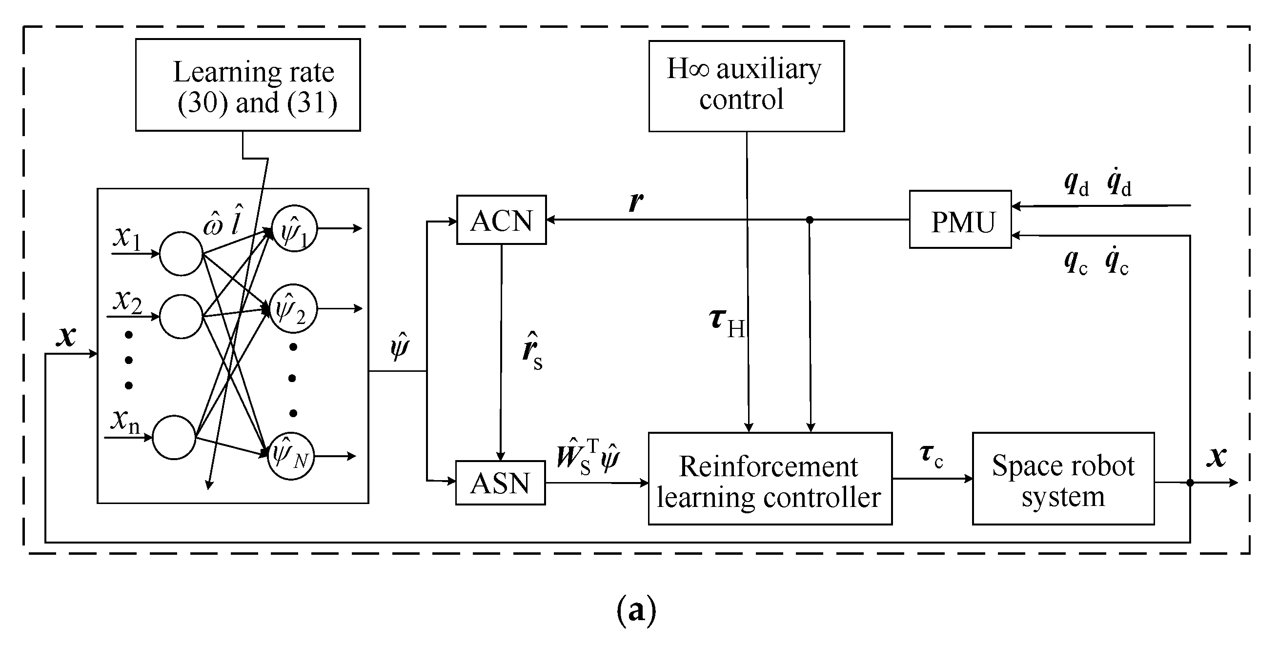
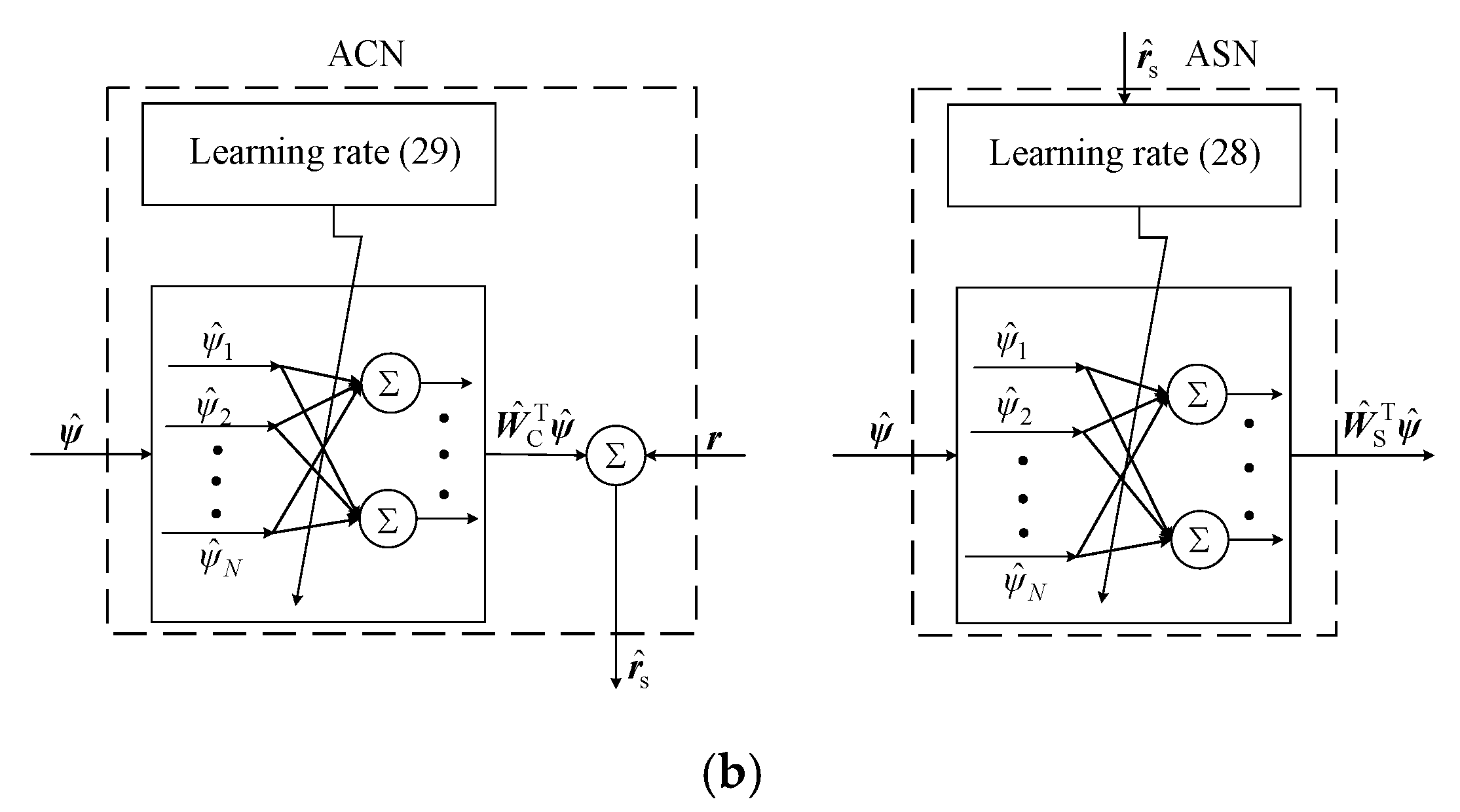
4. Design of Controller

The controller consists of a PMU, an ASN, and an ACN. Since the primary reinforcement signal is used to design the control torque directly, it easily leads to failure of stability control. Therefore, the controller obtains the primary reinforcement signal through the PMU, in turn using the ACN to construct a more informative signal than the primary reinforcement alone in order to tune the ASN realize stability control of the hybrid system. The control based on fuzzy logic RL is shown in Figure 4.

Property 1.

The matrix ${\dot{\mathit{M}}}_{\mathrm{h}}(q_{\mathrm{h}})$ and $H_{\mathrm{h}}(q_{\mathrm{h}},{\dot{\mathit{q}}}_{\mathrm{h}})$ are skew symmetric matrix such that $\frac{1}{2}{z}^{\mathrm{T}}{\dot{\mathit{M}}}_{\mathrm{h}}(q_{\mathrm{h}})z=z^{\mathrm{T}}{H}_{\mathrm{h}}(q_{\mathrm{h}},{\dot{\mathit{q}}}_{\mathrm{h}})z$, where $z\in R^{n+1}$ is the arbitrary column vector.

Assumption 1.

The matrix $M_{\mathrm{h}}(q_{\mathrm{h}})$ and $H_{\mathrm{h}}(q_{\mathrm{h}},{\dot{\mathit{q}}}_{\mathrm{h}})$ are bounded such that $‖H_{\mathrm{h}}(q_{\mathrm{h}},{\dot{\mathit{q}}}_{\mathrm{h}}){\dot{\mathit{q}}}_{\mathrm{h}}‖\le {\lambda }_{\mathrm{H}}‖{\dot{\mathit{q}}}_{\mathrm{h}}‖$, ${\lambda }_{\mathrm{m}}\le ‖M_{\mathrm{h}}(q_{\mathrm{h}})‖\le {\lambda }_{\mathrm{M}}$, where ${\lambda }_{\mathrm{m}}$, ${\lambda }_{\mathrm{M}}$ and ${\lambda }_{\mathrm{H}}$ are positive constants.

The position error and performance measurement signal are defined as follows:

$$e=q_{\mathrm{d}}-q_{\mathrm{h}}$$

(14)

$$S=\dot{\mathit{e}}+\Lambda e$$

(15)

where $\Lambda =\mathrm{diag}({\Lambda }_1,{\Lambda }_2,\cdot \cdot \cdot ,{\Lambda }_{n+1})$ is a diagonal matrix.

The primary reinforcement signal can be obtained from Equations (14) and (15):

$$r(t)=L\sigma (t)$$

(16)

where $L=\mathrm{diag}(\frac{1}{{\rho }_1},\frac{1}{{\rho }_2},\cdot \cdot \cdot ,\frac{1}{{\rho }_{n+1}}),{\rho }_i>0,(i=1,2,\cdot \cdot \cdot ,n+1)$, $\sigma (t)=[{\sigma }_1(s_1(t)),{\sigma }_2(s_2(t))$, $\cdot \cdot \cdot ,{\sigma }_{n+1}(s_{n+1}(t)){]}^{\mathrm{T}}$, ${\sigma }_i(s_i(t))=\frac{e^{{\rho }_i{s}_i(t)}-e^{-{\rho }_i{s}_i(t)}}{e^{{\rho }_i{s}_i(t)}+e^{-{\rho }_i{s}_i(t)}},(i=1,2,\cdot \cdot \cdot ,n+1)$. Then,

$$M_{\mathrm{h}}\dot{\mathit{r}}=-(H_{\mathrm{h}}+D_{\mathrm{Lh}})r-{\tau }_{\mathrm{h}}+\chi (x)$$

(17)

where $\chi (x)=M_{\mathrm{h}}[{\ddot{\mathit{q}}}_{\mathrm{d}}+\mathit{\Lambda }\dot{\mathit{e}}-\mathrm{diag}({\sigma }^2)(\ddot{\mathit{e}}+\mathit{\Lambda }\dot{\mathit{e}})]+H_{\mathrm{h}}({\dot{\mathit{q}}}_{\mathrm{d}}-\dot{\mathit{e}}+r)$, $x={[q_{\mathrm{h}},{\dot{\mathit{q}}}_{\mathrm{h}},{\ddot{\mathit{q}}}_{\mathrm{h}},q_{\mathrm{d}},{\dot{\mathit{q}}}_{\mathrm{d}},{\ddot{\mathit{q}}}_{\mathrm{d}}]}^{\mathrm{T}}$ is the uncertain item in system.

In order to eliminate the influence of uncertain item on control accuracy, ASN is used to estimate the controller of wavelet neural network. It is assumed that the estimation of uncertain item by wavelet neural network is as follows:

$$\widehat{\chi }={\widehat{W}}_{\mathrm{S}}^{\mathrm{T}}\psi (x,\widehat{l},\widehat{\mathit{\varpi }})$$

(18)

where ${\widehat{W}}_{\mathrm{S}}=[{\widehat{w}}_{\mathrm{S}1},{\widehat{w}}_{\mathrm{S}2},\cdot \cdot \cdot ,{\widehat{w}}_{\mathrm{S}m}]$ is the estimates of the weight matrix.

Based on this, the control signals are designed as follow:

$${\tau }_{\mathrm{h}}=K_{\mathrm{r}}r+\widehat{\chi }+{\tau }_{\mathrm{H}}$$

(19)

where $K_{\mathrm{r}}\in R^{(n+1)\times (n+1)}$ is a positive definite diagonal matrix, ${\tau }_{\mathrm{H}}=\frac{1}{k_{\mathrm{d}}}r,k_{\mathrm{d}}>0$.

Combine Equations (17) and (19) to get:

$$M_{\mathrm{h}}\dot{r}=-(K_{\mathrm{r}}+H_{\mathrm{h}}+D_{\mathrm{Lh}})r+\tilde{\chi }(x)-{\tau }_{\mathrm{H}}$$

(20)

where $\tilde{\chi }=\chi -\widehat{\chi }$.

The primary reinforcement signal can be enhanced as follows:

$$r_{\mathrm{s}}(t)=r(t)+\Gamma W_{\mathrm{C}}^{*\mathrm{T}}(t){\psi }^{*}(t)$$

(21)

where $W_{\mathrm{C}}^{*}$ is the ideal weight matrix, ${\psi }^{*}$ is the ideal regression matrix, $\Gamma =\mathrm{diag}(r_{\mathrm{s}1},r_{\mathrm{s}2},\cdot \cdot \cdot ,r_{\mathrm{s},n+1})$ and $r_{\mathrm{s}i}$ is the element in $r_{\mathrm{s}}$.

It is assumed that the enhancement signal can be approximated by ACN as follows:

$${\widehat{r}}_{\mathrm{s}}(t)=r(t)+\Gamma {\widehat{W}}_{\mathrm{C}}^{\mathrm{T}}(t)\widehat{\psi }(t)$$

(22)

where ${\widehat{W}}_{\mathrm{C}}=[{\widehat{w}}_{\mathrm{C}1},{\widehat{w}}_{\mathrm{C}2},\cdot \cdot \cdot ,{\widehat{w}}_{\mathrm{C}m}]$ is the estimated value of weight matrix, and $\widehat{\psi }$ is the estimated value of regression matrix. Expand $\tilde{\psi }={\psi }^{*}-\widehat{\psi }$ by Taylor as follows:

$$\tilde{\psi }={\left.\left[\begin{array}{c}{\left(\frac{\partial {\psi }_1}{\partial \mathit{\varpi }}\right)}^{\mathrm{T}}\\ ⋮\\ {\left(\frac{\partial {\psi }_N}{\partial \mathit{\varpi }}\right)}^{\mathrm{T}}\end{array}\right]\right|}_{\mathit{\varpi }=\widehat{\mathit{\varpi }}}\tilde{\mathit{\varpi }}+{\left.\left[\begin{array}{c}{\left(\frac{\partial {\psi }_1}{\partial l}\right)}^{\mathrm{T}}\\ ⋮\\ {\left(\frac{\partial {\psi }_N}{\partial l}\right)}^{\mathrm{T}}\end{array}\right]\right|}_{l=\widehat{l}}\tilde{l}+\xi$$

(23)

where $\tilde{\mathit{\varpi }}={\mathit{\varpi }}^{*}-\widehat{\mathit{\varpi }}$, $\tilde{l}=l^{*}-\widehat{l}$. The Equation (23) can be rewritten as:

$$\tilde{\psi }={\mathbf{\alpha }}^{\mathrm{T}}\tilde{\mathit{\varpi }}+{\beta }^{\mathrm{T}}\tilde{l}+\xi$$

(24)

Assumption 2.

The ideal weight $w_{\mathrm{C}k}^{*}$ and ${\mathit{\varpi }}_j^{*}$, centre value $l_j^{*}$, and width ${\mathit{\varpi }}_j^{*}$ of fuzzy wavelet neural network are bounded such that $0<‖w_{\mathrm{C}k}^{*}‖\le b_{wck}$, $0<‖w_{Sk}^{*}‖\le b_{sck}$, $0<‖{\mathit{\varpi }}_j^{*}‖\le b_{\omega j}$, $0<‖l_j^{*}‖\le b_{lj}$, $k=1,2,\cdot \cdot \cdot ,m$, $j=1,2,\cdot \cdot \cdot ,N$.

Assumption 3.

The Taylor remainder $\xi$, $\partial {\psi }_j/\partial \mathit{\varpi }$ and $\partial {\psi }_j/\partial l$ are bounded such that $‖\xi ‖\le b_{\xi }$, $\partial {\psi }_j/\partial \mathit{\varpi }\le b_{\eta j}$, $\partial {\psi }_j/\partial \mathit{\varpi }\le b_{\kappa j}$.

Combined with Equation (24), the output of ACN can be expressed as follows:

$${\widehat{W}}_{\mathrm{C}}^{\mathrm{T}}\widehat{\psi }=-{\tilde{W}}_{\mathrm{C}}^{\mathrm{T}}(\widehat{\psi }-{\mathbf{\alpha }}^{\mathrm{T}}\widehat{\mathit{\varpi }}-{\mathbf{\beta }}^{\mathrm{T}}\widehat{\mathbf{l}})-{\widehat{W}}_{\mathrm{C}}^{\mathrm{T}}({\mathbf{\alpha }}^{\mathrm{T}}\tilde{\mathit{\varpi }}+{\mathbf{\beta }}^{\mathrm{T}}\tilde{\mathbf{l}})-{\upsilon }_1$$

(25)

where ${\upsilon }_1=W_{\mathrm{C}}^{*\mathrm{T}}({\psi }^{*}-{\mathbf{\alpha }}^{\mathrm{T}}{\mathit{\varpi }}^{*}-{\beta }^{\mathrm{T}}{l}^{*}-\xi )-{\widehat{W}}_{\mathrm{C}}^{\mathrm{T}}({\mathbf{\alpha }}^{\mathrm{T}}{\mathit{\varpi }}^{*}+{\beta }^{\mathrm{T}}{l}^{*})$, ${\tilde{W}}_{\mathrm{C}}=W_{\mathrm{C}}^{*}-{\widehat{W}}_{\mathrm{C}}$. Then:

$$\chi -{\widehat{W}}_{\mathrm{C}}^{\mathrm{T}}\widehat{\psi }={\Xi }_{\chi }+W_{\mathrm{S}}^{*\mathrm{T}}\tilde{\psi }+{\tilde{W}}_{\mathrm{S}}^{\mathrm{T}}\widehat{\psi }$$

(26)

where ${\tilde{W}}_{\mathrm{S}}=W_{\mathrm{S}}^{*}-{\widehat{W}}_{\mathrm{S}}$, ${\Xi }_{\chi }=\chi -W_{\mathrm{S}}^{*\mathrm{T}}{\psi }^{*}$.

Combined with Equation (26), the Equation (20) can be rewrite:

$$M_{\mathrm{h}}\dot{\mathbf{r}}=-(K_{\mathrm{r}}+H_{\mathrm{h}}+D_{\mathrm{Lh}})r+{\Xi }_{\chi }+W_{\mathrm{S}}^{*\mathrm{T}}\tilde{\psi }+{\tilde{W}}_{\mathrm{S}}^{\mathrm{T}}\widehat{\psi }-{\tau }_{\mathrm{H}}$$

(27)

The adaptive rate of ASN and ACN are designed as follows:

$${\dot{\widehat{\mathbf{w}}}}_{Sk}=k_{wsk}({\widehat{r}}_{sk}+{\widehat{r}}_{sk}{\widehat{w}}_{Ck}^{\mathrm{T}}\widehat{\psi })\left(\widehat{\psi }-I_{sk}\frac{{\widehat{w}}_{Sk}{\widehat{w}}_{Sk}^{\mathrm{T}}\widehat{\psi }}{{‖{\widehat{w}}_{Sk}‖}^2}\right)$$

(28)

$${\dot{\widehat{\mathbf{w}}}}_{Ck}=-k_{wck}{\widehat{r}}_{sk}({\widehat{w}}_{Sk}^{\mathrm{T}}\widehat{\psi })\left((\widehat{\psi }-{\mathbf{\alpha }}^{\mathrm{T}}\widehat{\mathit{\varpi }}-{\beta }^{\mathrm{T}}\widehat{l})-\right.\left. I_{ck}\frac{{\widehat{w}}_{Ck}{\widehat{w}}_{Ck}^{\mathrm{T}}(\widehat{\psi }-{\mathbf{\alpha }}^{\mathrm{T}}\widehat{\mathit{\varpi }}-{\beta }^{\mathrm{T}}\widehat{l})}{{‖{\widehat{w}}_{Ck}‖}^2}\right)$$

(29)

$$\dot{\widehat{\mathit{\varpi }}}=-k_{\omega }\left(A{\widehat{W}}_{\mathrm{C}}\Gamma {\widehat{W}}_{\mathrm{S}}^{\mathrm{T}}\widehat{\psi }-I_{\omega }\frac{\widehat{\omega }{\widehat{\omega }}^{\mathrm{T}}(A{\widehat{W}}_{\mathrm{C}}\Gamma {\widehat{W}}_{\mathrm{S}}^{\mathrm{T}}\widehat{\psi })}{{‖\widehat{\mathit{\varpi }}‖}^2}\right)$$

(30)

$$\dot{\widehat{l}}=-k_l\left(B{\widehat{W}}_{\mathrm{C}}\Gamma {\widehat{W}}_{\mathrm{S}}^{\mathrm{T}}\widehat{\psi }-I_l\frac{\widehat{l}{\widehat{l}}^{\mathrm{T}}(B{\widehat{W}}_{\mathrm{C}}\Gamma {\widehat{W}}_{\mathrm{S}}^{\mathrm{T}}\widehat{\psi })}{{‖\widehat{l}‖}^2}\right)$$

(31)

where $k_{wsk}$, $k_{wck}$, $k_{\omega }$ and $k_l$ are positive constants, and the value of $I_{sk}$, $I_{ck}$, $I_{\omega }$ and $I_l$ are as follows:

$$I_{sk}=\left\{\begin{array}{l}0 \mathrm{if} (‖{\widehat{w}}_{Sk}‖<b_{wsk}) \mathrm{or} (‖{\widehat{w}}_{Sk}‖=b_{wsk}, ({\widehat{r}}_{sk}+{\widehat{r}}_{sk}{\widehat{w}}_{Ck}^{\mathrm{T}}\widehat{\psi }){\widehat{w}}_{Sk}^{\mathrm{T}}\widehat{\psi }\le 0)\\ 1 \mathrm{if} (‖{\widehat{w}}_{Sk}‖=b_{wsk},({\widehat{r}}_{sk}+{\widehat{r}}_{sk}{\widehat{w}}_{Ck}^{\mathrm{T}}\widehat{\psi }){\widehat{w}}_{Sk}^{\mathrm{T}}\widehat{\psi }>>0)\end{array}\right.$$

(32)

$$I_{ck}=\left\{\begin{array}{l}0 \mathrm{if} (‖{\widehat{w}}_{Ck}‖<<b_{wck}) \mathrm{or} (‖{\widehat{w}}_{Ck}‖=b_{wck}, {\widehat{r}}_{sk}({\widehat{w}}_{Sk}^{\mathrm{T}}\widehat{\psi }){\widehat{w}}_{Ck}^{\mathrm{T}}((\widehat{\psi }-{\mathbf{\alpha }}^{\mathrm{T}}\widehat{\mathit{\varpi }}-{\beta }^{\mathrm{T}}\widehat{l}))\ge 0)\\ 1 \mathrm{if} (‖{\widehat{w}}_{Sk}‖=b_{wck},{\widehat{r}}_{sk}({\widehat{w}}_{Sk}^{\mathrm{T}}\widehat{\psi }){\widehat{w}}_{Ck}^{\mathrm{T}}((\widehat{\psi }-{\mathbf{\alpha }}^{\mathrm{T}}\widehat{\mathit{\varpi }}-{\beta }^{\mathrm{T}}\widehat{l}))<<0)\end{array}\right.$$

(33)

$$I_{\omega }=\left\{\begin{array}{l}0 \mathrm{if} (‖\widehat{\mathit{\varpi }}‖<<b_{\mathit{\varpi }}) \mathrm{or} (‖\widehat{\mathit{\varpi }}‖=b_{\mathit{\varpi }},{\widehat{\mathit{\varpi }}}^{\mathrm{T}}(A{\widehat{W}}_{\mathrm{C}}\Gamma {\widehat{W}}_{\mathrm{S}}^{\mathrm{T}}\widehat{\psi })\ge 0)\\ 1 \mathrm{if} ‖\widehat{\mathit{\varpi }}‖=b_{\mathit{\varpi }},{\widehat{\mathit{\varpi }}}^{\mathrm{T}}(A{\widehat{W}}_{\mathrm{C}}\Gamma {\widehat{W}}_{\mathrm{S}}^{\mathrm{T}}\widehat{\psi })<<0)\end{array}\right.$$

(34)

$$I_l=\left\{\begin{array}{l}0 \mathrm{if} (‖\widehat{l}‖<<b_l) \mathrm{or} (‖\widehat{l}‖=b_l,{\widehat{l}}^{\mathrm{T}}(B{\widehat{W}}_{\mathrm{C}}\Gamma {\widehat{W}}_{\mathrm{S}}^{\mathrm{T}}\widehat{\psi })\ge 0)\\ 1 \mathrm{if} ‖\widehat{l}‖=b_l,{\widehat{l}}^{\mathrm{T}}\left(B{\widehat{W}}_{\mathrm{C}}\Gamma {\widehat{W}}_{\mathrm{S}}^{\mathrm{T}}\widehat{\psi }\right)<<0)\end{array}\right.$$

(35)

Theorem 1.

For the hybrid system dynamic mode of the Equation (13), supposing that Assumptions 1 to 3 hold and adopting the error evaluation signal shown in Equation (15), the control signal shown in Equation (19), the reinforcement signal shown in Equations (16) and (21), and the update rate of fuzzy wavelet neural network shown in Equations (28)–(31) can ensure that the trajectory tracking error $e$ converges to zero asymptotically.

Proof of Theorem 1.

Introducing the Lyapunov function:

$$V=\frac{1}{2}{r}^{\mathrm{T}}{M}_{\mathrm{h}}r+\frac{1}{2}{\displaystyle \sum _{k=1}^m\frac{1}{k_{wsk}}}{\tilde{w}}_{Sk}^{\mathrm{T}}{\tilde{w}}_{Sk}+\frac{1}{2}{\displaystyle \sum _{k=1}^m\frac{1}{k_{wck}}}{\tilde{w}}_{Ck}^{\mathrm{T}}{\tilde{w}}_{Ck}+\frac{1}{2k_{\omega }}{\tilde{\omega }}^{\mathrm{T}}\tilde{\omega }+\frac{1}{2k_l}{\tilde{l}}^{\mathrm{T}}\tilde{l}$$

(36)

Then, derivative of the Equation (36)

$$\dot{V}=r^{\mathrm{T}}{M}_{\mathrm{h}}\dot{r}+\frac{1}{2}{r}^{\mathrm{T}}{\dot{M}}_{\mathrm{h}}r-{\displaystyle \sum _{k=1}^m\frac{1}{k_{wsk}}}{\tilde{w}}_{Sk}^{\mathrm{T}}{\dot{\widehat{w}}}_{Sk}-{\displaystyle \sum _{k=1}^m\frac{1}{k_{wck}}}{\tilde{w}}_{Ck}^{\mathrm{T}}{\dot{\widehat{w}}}_{Ck}-\frac{1}{k_{\omega }}{\tilde{\omega }}^{\mathrm{T}}\dot{\widehat{\omega }}-\frac{1}{k_l}{\tilde{l}}^{\mathrm{T}}\dot{\widehat{l}}$$

(37)

Combined with Property 1 and Equations (27)–(29), the Equation (37) can be rewrite:

$$\begin{array}{cc}\dot{V}=& r^{\mathrm{T}}({\Xi }_{\chi }+W_{\mathrm{S}}^{*\mathrm{T}}\tilde{\psi })-r^{\mathrm{T}}{\tau }_{\mathrm{H}}-{(W_{\mathrm{S}}^{*\mathrm{T}}\widehat{\psi })}^{\mathrm{T}}\Gamma {\widehat{W}}_{\mathrm{C}}^{\mathrm{T}}\widehat{\psi }+{({\widehat{W}}_{\mathrm{S}}^{\mathrm{T}}\widehat{\psi })}^{\mathrm{T}}\Gamma {\widehat{W}}_{\mathrm{C}}^{\mathrm{T}}\widehat{\psi }-\hfill \\ & {\displaystyle \sum _{k=1}^m(r_{sk}+r_{sk}{\widehat{w}}_{Ck}^{\mathrm{T}}\widehat{\psi })I_{sk}\frac{{\tilde{w}}_{Sk}^{\mathrm{T}}{\widehat{w}}_{Sk}{\widehat{w}}_{Sk}^{\mathrm{T}}\widehat{\psi }}{{‖{\widehat{w}}_{Sk}‖}^2}-r^{\mathrm{T}}{K}_{\mathrm{DLr}}r-\frac{1}{k_{\omega }}{\tilde{\omega }}^{\mathrm{T}}\dot{\widehat{\omega }}-\frac{1}{k_l}{\tilde{l}}^{\mathrm{T}}\dot{\widehat{l}}+}\hfill \\ & {\displaystyle \sum _{k=1}^m{r}_{sk}({\widehat{w}}_{Sk}^{\mathrm{T}}\widehat{\psi })\left({\tilde{w}}_{Ck}^{\mathrm{T}}(\widehat{\psi }-{\mathbf{\alpha }}^{\mathrm{T}}\widehat{\mathit{\varpi }}-{\beta }^{\mathrm{T}}\widehat{l})-I_{ck}\frac{{\tilde{w}}_{Ck}^{\mathrm{T}}{\widehat{w}}_{Ck}{\widehat{w}}_{Ck}^{\mathrm{T}}(\widehat{\psi }-{\mathbf{\alpha }}^{\mathrm{T}}\widehat{\mathit{\varpi }}-{\beta }^{\mathrm{T}}\widehat{l})}{{‖{\widehat{w}}_{Ck}‖}^2}\right)}\hfill \end{array}$$

(38)

where $K_{\mathrm{DLr}}=K_{\mathrm{r}}+D_{\mathrm{Lc}}$. Substituting Equations (26), (30) and (31) into Equation (38) can obtain:

$$\begin{array}{cc}\dot{V}=& -{(W_{\mathrm{S}}^{*\mathrm{T}}\widehat{\psi })}^{\mathrm{T}}\Gamma {\widehat{W}}_{\mathrm{C}}^{\mathrm{T}}\widehat{\psi }-{({\widehat{W}}_{\mathrm{S}}^{\mathrm{T}}\widehat{\psi })}^{\mathrm{T}}\Gamma \left[{\tilde{W}}_{\mathrm{C}}^{\mathrm{T}}(\widehat{\psi }-\right.\left.{\mathbf{\alpha }}^{\mathrm{T}}\widehat{\mathit{\varpi }}-{\beta }^{\mathrm{T}}\widehat{l})+{\widehat{W}}_{\mathrm{C}}^{\mathrm{T}}({\mathbf{\alpha }}^{\mathrm{T}}\tilde{\mathit{\varpi }}+{\beta }^{\mathrm{T}}\tilde{l})+{\Xi }_{\chi }\right]-\hfill \\ & r^{\mathrm{T}}{K}_{\mathrm{DLr}}r+r^{\mathrm{T}}({\Xi }_{\chi }+W_{\mathrm{S}}^{*\mathrm{T}}\tilde{\psi })-r^{\mathrm{T}}{\tau }_{\mathrm{H}}+{\displaystyle \sum _{k=1}^m(r_{sk}+r_{sk}{\widehat{w}}_{Ck}^{\mathrm{T}}\widehat{\psi })I_{sk}\frac{{\tilde{w}}_{Sk}^{\mathrm{T}}{\widehat{w}}_{Sk}{\widehat{w}}_{Sk}^{\mathrm{T}}\widehat{\psi }}{{‖{\widehat{w}}_{Sk}‖}^2}+}\hfill \\ & {\displaystyle \sum _{k=1}^m{r}_{sk}({\widehat{w}}_{Sk}^{\mathrm{T}}\widehat{\psi })}\left({\tilde{w}}_{Ck}^{\mathrm{T}}(\widehat{\psi }-{\mathbf{\alpha }}^{\mathrm{T}}\widehat{\mathit{\varpi }}-{\beta }^{\mathrm{T}}\widehat{l})-I_{ck}\frac{{\tilde{w}}_{Ck}^{\mathrm{T}}{\widehat{w}}_{Ck}{\widehat{w}}_{Ck}^{\mathrm{T}}(\widehat{\psi }-{\mathbf{\alpha }}^{\mathrm{T}}\widehat{\mathit{\varpi }}-{\beta }^{\mathrm{T}}\widehat{l})}{{‖{\widehat{w}}_{Ck}‖}^2}\right)+\hfill \\ & {\tilde{\mathit{\varpi }}}^{\mathrm{T}}(\left(A{\widehat{W}}_{\mathrm{C}}\Gamma {\widehat{W}}_{\mathrm{S}}^{\mathrm{T}}\widehat{\psi }-I_{\omega }\frac{\widehat{\omega }{\widehat{\omega }}^{\mathrm{T}}(A{\widehat{W}}_{\mathrm{C}}\Gamma {\widehat{W}}_{\mathrm{S}}^{\mathrm{T}}\widehat{\psi })}{{‖\widehat{\mathit{\varpi }}‖}^2}\right)+{\tilde{l}}^{\mathrm{T}}\left(B{\widehat{W}}_{\mathrm{C}}\Gamma {\widehat{W}}_{\mathrm{S}}^{\mathrm{T}}\widehat{\psi }-I_l\frac{\widehat{l}{\widehat{l}}^{\mathrm{T}}(B{\widehat{W}}_{\mathrm{C}}\Gamma {\widehat{W}}_{\mathrm{S}}^{\mathrm{T}}\widehat{\psi })}{{‖\widehat{l}‖}^2}\right)\hfill \end{array}$$

(39)

Based on Assumption 2, Assumption 3 and Equations (32)–(35) to obtain:

$$\begin{gathered} I_{sk}(r_{sk}+r_{sk}{\widehat{w}}_{Ck}^{\mathrm{T}}\widehat{\psi }){\tilde{w}}_{Sk}^{\mathrm{T}}{\widehat{w}}_{Sk}{\widehat{w}}_{Sk}^{\mathrm{T}}\widehat{\psi }/{‖{\widehat{w}}_{Sk}‖}^2\le 0 \\ {r}_{sk}({\widehat{w}}_{Sk}^{\mathrm{T}}\widehat{\psi })\left(I_{ck}{\tilde{w}}_{Ck}^{\mathrm{T}}{\widehat{w}}_{Ck}{\widehat{w}}_{Ck}^{\mathrm{T}}(\widehat{\psi }-{\mathbf{\alpha }}^{\mathrm{T}}\widehat{\mathit{\varpi }}-{\beta }^{\mathrm{T}}\widehat{l})/{‖{\widehat{w}}_{Ck}‖}^2\right)\ge 0 \\ {I}_{\omega }\left({\tilde{\mathit{\varpi }}}^{\mathrm{T}}\widehat{\omega }{\widehat{\omega }}^{\mathrm{T}}(A{\widehat{W}}_{\mathrm{C}}\Gamma {\widehat{W}}_{\mathrm{S}}^{\mathrm{T}}\widehat{\psi })/{‖\widehat{\mathit{\varpi }}‖}^2\right)\ge 0 \\ {I}_l\left({\tilde{l}}^{\mathrm{T}}\widehat{l}{\widehat{l}}^{\mathrm{T}}(B{\widehat{W}}_{\mathrm{C}}\Gamma {\widehat{W}}_{\mathrm{S}}^{\mathrm{T}}\widehat{\psi })/{‖\widehat{l}‖}^2\right)\ge 0 \end{gathered}$$

Then

$$\begin{array}{l}\dot{V}\le -r^{\mathrm{T}}{K}_{\mathrm{DLr}}r+r^{\mathrm{T}}({\Xi }_{\chi }+W_{\mathrm{S}}^{*\mathrm{T}}\tilde{\psi })-r^{\mathrm{T}}{\tau }_{\mathrm{H}}+{(W_{\mathrm{S}}^{*\mathrm{T}}\widehat{\psi })}^{\mathrm{T}}\Gamma {\widehat{W}}_{\mathrm{C}}^{\mathrm{T}}\widehat{\psi }-{({\widehat{W}}_{\mathrm{S}}^{\mathrm{T}}\widehat{\psi })}^{\mathrm{T}}\Gamma {\upsilon }_1\\ \le -r^{\mathrm{T}}{K}_{\mathrm{DLr}}r+r^{\mathrm{T}}\upsilon -r^{\mathrm{T}}{\tau }_{\mathrm{H}}\end{array}$$

(40)

where $\upsilon ={\Xi }_{\chi }+W_{\mathrm{S}}^{*\mathrm{T}}\tilde{\psi }+\mathrm{diag}(W_{\mathrm{S}}^{*\mathrm{T}}\widehat{\psi }){\widehat{W}}_{\mathrm{C}}^{\mathrm{T}}\widehat{\psi }-\mathrm{diag}({\widehat{W}}_{\mathrm{S}}^{\mathrm{T}}\widehat{\psi }){\upsilon }_1$.

The Equation (40) can be rewrite:

$$\begin{array}{l}\dot{V}\le -\frac{1}{2}{r}^{\mathrm{T}}\left[2K_{\mathrm{DLr}}+(\frac{2}{k_{\mathrm{d}}}-\frac{1}{{\gamma }^2})E\right]r-\frac{1}{2}{(\frac{1}{\gamma }r-\gamma \upsilon )}^{\mathrm{T}}(\frac{1}{\gamma }r-\gamma \upsilon )+\frac{1}{2}{\gamma }^2{\upsilon }^{\mathrm{T}}\upsilon \\ \le -\frac{1}{2}{r}^{\mathrm{T}}Qr+\frac{1}{2}{\gamma }^2{\upsilon }^{\mathrm{T}}\upsilon \end{array}$$

(41)

where $Q=2K_{\mathrm{DLr}}+(2/k_{\mathrm{d}}-1/{\gamma }^2)E$ is a positive definite diagonal matrix, $E$ is a unit matrix.

By integrating Equation (41) to obtain:

$$V(T)-V(0)\le \frac{1}{2}{\displaystyle {\int }_0^T{r}^{\mathrm{T}}Qrdt}+\frac{1}{2}{\gamma }^2{\displaystyle {\int }_0^T{\upsilon }^{\mathrm{T}}\upsilon dt}$$

(42)

Then

$$\begin{array}{l}{\displaystyle {\int }_0^T{r}^{\mathrm{T}}Qrdt}\le r{(0)}^{\mathrm{T}}{M}_{\mathrm{c}}r(0)+{\displaystyle \sum _{k=1}^m\frac{1}{k_{wsk}}}{\tilde{w}}_{Sk}^{\mathrm{T}}(0){\tilde{w}}_{Sk}(0)+{\displaystyle \sum _{k=1}^m\frac{1}{k_{wck}}}{\tilde{w}}_{Ck}^{\mathrm{T}}(0){\tilde{w}}_{Ck}(0)+\\ \frac{1}{k_{\omega }}{\tilde{\omega }}^{\mathrm{T}}(0)\tilde{\omega }(0)+ \frac{1}{k_l}{\tilde{l}}^{\mathrm{T}}(0)\tilde{l}(0)+{\gamma }^2{\displaystyle {\int }_0^T{\upsilon }^{\mathrm{T}}\upsilon dt}\end{array}$$

(43)

Equation (43) can be written in the following form through references [37,38].

$${\displaystyle {\int }_0^T{‖r‖}^2}Qdt\le {\gamma }^2{\displaystyle {\int }_0^T{‖\upsilon ‖}^{2}dt}+{\beta }_{\mathrm{H}}$$

(44)

where ${\beta }_{\mathrm{H}}=r{(0)}^{\mathrm{T}}{M}_{\mathrm{c}}r(0)+{\displaystyle \sum _{k=1}^m\frac{1}{k_{wsk}}}{\tilde{w}}_{Sk}^{\mathrm{T}}(0){\tilde{w}}_{Sk}(0)+{\displaystyle \sum _{k=1}^m\frac{1}{k_{wck}}}{\tilde{w}}_{Ck}^{\mathrm{T}}(0){\tilde{w}}_{Ck}(0)+\frac{1}{k_{\omega }}{\tilde{\omega }}^{\mathrm{T}}(0)\tilde{\omega }(0)+\frac{1}{k_l}{\tilde{l}}^{\mathrm{T}}(0)\tilde{l}(0)$.

Through references [37,38], It can be known that $\upsilon$ is bounded by Assumption 1 and Assumption 2, further $\underset{\upsilon \in L_2[0,T]}{\sup }{‖Q^{1/2}r‖}_{L2T}/{‖\upsilon ‖}_{L2T}\le \gamma$ when the initial states of the hybrid system are all zero. According to the definition of Q in Equation (41), it can be explained that the system is stable according to the $H\infty$ control theory when $k_{\mathrm{d}}=2{\gamma }^2$, and it can be seen that with the decrease of $\gamma$, $‖r‖$ will also decrease. □

5. Simulation Results

5.1. Simulation of Impact Resistance of the SDD

Using the two-link space robot ($n=2$) and satellite systems in Figure 3 for simulation analysis. The initial position and velocity of space robot are $q(0)={[1.75,0.52,1.05]}^{\mathrm{T}}$ rad, $\dot{\mathit{q}}(0)={[0,0,0]}^{\mathrm{T}}$ rad/s. The actual parameters of space robot and satellite systems are as follow: $m_0=100 \mathrm{kg}$, $m_1=m_2=10 \mathrm{kg}$, $m_{\mathrm{s}}=50 \mathrm{kg}$, $L_0=1 \mathrm{m}$, $L_1=L_2=2 \mathrm{m}$, $d_1=d_2=1 \mathrm{m}$, $d_{\mathrm{s}}=0.5 \mathrm{m}$, $I_0=64 \mathrm{kg}\cdot {\mathrm{m}}^2$, $I_1=I_2=3.5 \mathrm{kg}\cdot {\mathrm{m}}^2$, $I_{\mathrm{m}1}=I_{\mathrm{m}2}=0.05 \mathrm{kg}\cdot {\mathrm{m}}^2$, $I_{\mathrm{s}}=12.5 \mathrm{kg}\cdot {\mathrm{m}}^2$, $k_{\mathrm{s}1}=k_{\mathrm{s}2}=1000 \mathrm{N}/\mathrm{rad}$, $D_{\mathrm{m}1}=D_{\mathrm{m}2}=28.65 \mathrm{N}\cdot \mathrm{s}/\mathrm{rad}$, $D_{\mathrm{t}1}=D_{\mathrm{t}2}=1146 \mathrm{N}\cdot \mathrm{s}/\mathrm{rad}$, $D_{\mathrm{L}1}=D_{\mathrm{L}2}=28.65 \mathrm{N}\cdot \mathrm{s}/\mathrm{rad}$.

In order to verify the impact resistance of the SDD during the third stage, the space robot system with/without SDD was used to carry out acquisition simulation tests on spacecraft with different velocity. The simulation results are shown in

Table 1. SDD impact resistance at different initial velocities of spacecraft.

Initial Velocity of Satellite/ (m/s, m/s, rad/s)	Max Impact Torque without SDD/ (N·m)	Max Impact Torque with SDD/ (N·m)	Percentage Reduction/ (%)
[0.1, 0.1, 0.15]T	226.68	133.27	41.21
[0.1, 0, 0]T	78.38	38.78	50.52
[0, 0.1, 0]T [0, 0, 0.15]T	34.17 117.33	15.67 66.09	54.14 43.67

.

As can be seen from Table 1, given different satellite velocities the SDD can significantly reduce the impact torque of joints, and the maximum can be reduced by 54.14%. Therefore, the SDD can be considered that it plays a good role in protecting joints during the third stage.

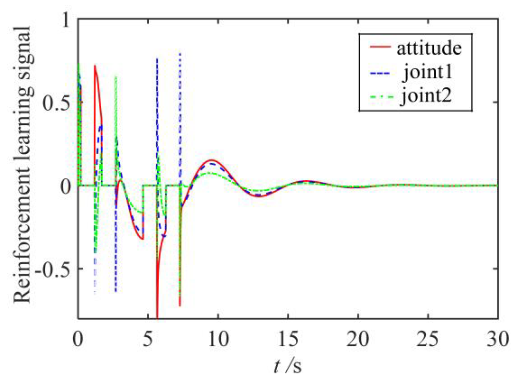
5.2. Buffer Compliance Control Strategy Performance Simulation

To show the buffer compliance control performance of the proposed controller, simulations are carried out for stable control phase. The actual parameters of the system are as follows:$\mathit{\Lambda }=\mathrm{diag}(2,2,2)$, ${\rho }_i=1.5(i=1,2,3)$, $K_{\mathrm{r}}=\mathrm{diag}(150,150,150)$, $\gamma =0.03$, $k_{wck}=3$, $k_{wsk}=3$, $k_{\mathit{\varpi }}=2$, $k_l=2$. The position of hybrid system after capture is $q(t_0)={[{84.61}^{\mathrm{o}}, {11.10}^{\mathrm{o}},{25.65}^{\mathrm{o}}]}^{\mathrm{T}}$, The initial position and velocity of space robot are the same as 5.1, the satellite initial velocity is ${\dot{q}}_{\mathrm{s}}(t_0)={[0.1 \mathrm{m}/\mathrm{s}, 0.1 \mathrm{m}/\mathrm{s}, 0.15 \mathrm{rad}/\mathrm{s}]}^{\mathrm{T}}$, and the expected state of hybrid system is $q_{\mathrm{d}}={[{100}^{\mathrm{o}},{30}^{\mathrm{o}},{60}^{\mathrm{o}}]}^{\mathrm{T}}$.

In order to highlight the advantages of SDD on SEA, the SEA structure of reference [3] is used for comparative analysis. In reference [3], to suppress the flexible vibration introduced by SEA, the controller is divided into a fast subsystem controller and slow subsystem controller, wherein the slow subsystem controller realizes trajectory tracking and the fast subsystem controller suppresses the flexible vibration. The simulation results are shown in Figure 5, Figure 6 and Figure 7.

It can be seen from Figure 5 and Figure 6 that under the same control parameters, whether in regards joint 1 or joint 2, adding SEA requires greater output torque than adding SDD, which means adding SEA will make the joint motor need more load capacity. Figure 7 shows that without the fast subsystem controller, the joint flexible vibration will be difficult to suppress and the joint angle fails to reach the desired state.

Assume that when the joint actuators run, the limit of the impact torque it can bear is $150 \mathrm{N}\cdot \mathrm{m}$. In order to protect the joint actuators, the buffer compliance control strategy of active opening and closing actuators (named switching strategy) is adopted. The shutdown torque threshold is $120 \mathrm{N}\cdot \mathrm{m}$, and the startup torque threshold is $10\mathrm{N}·\mathrm{m}$. The simulation results are shown in Figure 8, Figure 9, Figure 10 and Figure 11.

It can be seen from Figure 8 that the joint motor enters the stable output state after four shutdowns. Figure 9 shows that the RL controller can continuously output reinforcement signals when the base attitude angle and joint angle do not reach the desired position and reinforcement signal will to zero when they reach the desired position. Figure 10 shows that the ACN and ASN are optimized through the interaction with the environment and finally make the hybrid system reach a stable state. Figure 11 shows that the joint impact is limited to the bear torque well, and the buffer compliance strategy can realize the compliance of capture operation well.

Considering that the impact torque that the joint can bear will decrease with the increase of the space robot service years, the second group of simulation sets the shutdown torque threshold is $80 \mathrm{N}\cdot \mathrm{m}$, and the startup torque threshold is $10 \mathrm{N}\cdot \mathrm{m}$. The simulation results are shown in Figure 12, Figure 13, Figure 14 and Figure 15.

Figure 12 shows the joint motor enters the stable output state after seven shutdowns. As can be seen from Figure 12, Figure 13, Figure 14 and Figure 15, even if the shutdown torque threshold is lowered, the joint impact torque can be limited well within a safe range, and the RL controller can still complete the calm control of the unstable hybrid system by outputting the reinforcement signal. This means that the SDD has excellent protection performance for space robot joints, and it plays an important role in prolonging the service life of space robot.

6. Conclusions

In this paper, in order to protect the joints of a space robot from impact damage in the process of capturing satellite operation, an SDD is added between joint motor and manipulator, and a buffer compliance strategy that matches the SDD is given. The dynamic model of hybrid system is derived, and the impact effect and impact force are calculated during the third stage. For the purpose of realizing the stabilization control of the system, an RL control based on fuzzy wavelet neural network is proposed.

In the third stage of capture operation, a huge impact torque will be generated at the motor joint. Adding SDD between the motor and the manipulator can realize the rapid unloading of impact force, and the maximum value can be reduced by 54.14%.

In the fourth stage of capture operation (i.e., matching with the buffer compliance strategy designed by SDD), the joints’ impact torque can be limited to a safe range. The shutdown threshold of buffer compliance strategy can be set flexibly, which can protect the joints of space robot with different service years.

References

1. Fu, X.; Ai, H.; Chen, L. Repetitive learning sliding mode stabilization control for a flexible-base, flexible-link and flexible-joint space robot capturing a satellite. Appl. Sci. 2021, 11, 8077. [Google Scholar] [CrossRef]
2. He, J.; Zheng, H.; Gao, F.; Zhang, H. Dynamics and control of a 7-DOF hybrid manipulator for capturing a non-cooperative target in space. Mech. Machine Theory 2019, 140, 83–103. [Google Scholar] [CrossRef]
3. Ai, H.; Zhu, A.; Wang, J.; Yu, X.; Chen, L. Buffer Compliance Control of Space Robots Capturing a Non-Cooperative Spacecraft Based on Reinforcement Learning. Appl. Sci. 2021, 11, 5783. [Google Scholar] [CrossRef]
4. Meng, Q.; Liang, J.; Ma, O. Identification of all the inertial parameters of a non-cooperative object in orbit. Aerosp. Sci. Technol. 2019, 91, 571–582. [Google Scholar] [CrossRef]
5. Liu, X.; Li, H.; Chen, Y.; Cai, G. Dynamics and control of space robot considering joint friction. Acta Astronaut. 2015, 111, 1–18. [Google Scholar] [CrossRef]
6. Li, M.; Guo, W.; Lin, R.; Wu, C. An efficient motion generation method for redundant humanoid robot arms based on motion continuity. Adv. Robot. 2018, 32, 1185–1196. [Google Scholar] [CrossRef]
7. Fu, X.; Ai, H.; Chen, L. Integrated Fixed Time Sliding Mode Control for Motion and Vibration of Space Robot with Fully Flexible Base–Link–Joint. Appl. Sci. 2021, 11, 11685. [Google Scholar] [CrossRef]
8. Liu, X.; Li, H.; Chen, Y.; Cai, G.; Wang, X. Dynamics and control of capture of a floating rigid body by a spacecraft robotic arm. Multibody Syst. Dyn. 2015, 33, 315–332. [Google Scholar] [CrossRef]
9. Cheng, J.; Chen, L. Mechanical analysis and calm control of dual-arm space robot for capturing a satellite. Chin. J. Theor. Appl. Mech. 2016, 48, 832–842. (In Chinese) [Google Scholar]
10. Uyama, N.; Hirano, D.; Nakanishi, H.; Nagaoka, K.; Yoshida, K. Impedance-based contact control of a free-flying space robot with respect to coefficient of restitution. IEEE/SICE Int. Symp. Syst. Integr. 2012, 1196–1201. [Google Scholar] [CrossRef]
11. Dimitrov, D.; Yoshida, K. Utilization of the bias momentum approach for capturing a tumbling satellite. IEEE/RSJ Int. Conf. Intell. Robot. Syst. 2004, 3333–3338. [Google Scholar] [CrossRef]
12. Yoshida, K.; Nakanishi, H.; Ueno, H.; Inaba, N. Dynamics control and impedance matching for robotic capture of a non-cooperative satellite. Adv. Robot. 2004, 2, 175–198. [Google Scholar] [CrossRef]
13. Dong, Q.; Chen, L. Composite control of robust stabilization and adaptive vibration suppression of flexible space manipulator capturing a satellite. Robot 2014, 36, 342–348. (In Chinese) [Google Scholar]
14. Sariyildiz, E.; Chen, G.; Yu, H. An acceleration-based robust motion controller design for a novel series elastic actuator. IEEE Trans. Ind. Electron. 2016, 63, 1900–1910. [Google Scholar] [CrossRef]
15. Li, X.; Pan, Y.; Chen, G.; Yu, H. Continuous tracking control for a compliant actuator with two-stage stiffness. IEEE Trans. Autom. Sci. Eng. 2018, 15, 57–66. [Google Scholar] [CrossRef]
16. Lin, Y.; Chen, Z.; Yao, B. Decoupled torque control of series elastic actuator with adaptive robust compensation of time-varying load-side dynamics. IEEE Trans. Ind. Electron. 2019, 67, 5604–5614. [Google Scholar] [CrossRef]
17. Irmscher, C.; Woschke, E.; May, E.; Daniel, C. Design, Optimization and testing of a compact, inexpensive elastic element for series elastic actuators. Med. Eng. Phys. 2018, 52, 84–89. [Google Scholar] [CrossRef]
18. Keppler, M.; Lakatos, D.; Ott, C.; Albu-Schaffer, A. Elastic structure preserving (EPS) control for compliantly actuated robots. IEEE Trans. Robot. 2018, 34, 317–335. [Google Scholar] [CrossRef] [Green Version]
19. Yang, T.; Sun, N.; Fang, Y. Adaptive fuzzy control for a class of mimo underactuated systems with plant uncertainties and actuator deadzones: Design and experiments. IEEE Trans. Cybern. 2021, 99, 1–14. [Google Scholar] [CrossRef]
20. Sun, L.; Li, M.; Wang, M.; Yin, W.; Sun, N.; Liu, J. Continuous finite-time output torque control approach for series elastic actuator. Mech. Syst. Signal Processing 2020, 139, 105853. [Google Scholar] [CrossRef]
21. Wang, M.; Sun, L.; Yin, W.; Dong, S.; Liu, J. Continuous robust control for series elastic actuator with unknown payload parameters and external disturbances. IEEE/CAA J. Autom. Sin. 2017, 4, 620–627. [Google Scholar] [CrossRef]
22. Ai, H.; Chen, L. Buffer and compliant dynamic surface control of space robot capturing satellite based on compliant mechanism. Chin. J. Theor. Appl. Mech. 2020, 52, 975–984. (In Chinese) [Google Scholar]
23. Liu, S.; Wu, L.; Lu, Z. Impact dynamics and control of a flexible dual-arm space robot capturing an object. Appl. Math. Comput. 2007, 185, 1149–1159. [Google Scholar] [CrossRef]
24. Huang, X.; Duan, G. Attitude control and structure robust control allocation for combined spacecraft. Control. Theory Appl. 2018, 35, 1447–1457. (In Chinese) [Google Scholar]
25. Luo, J.; Wei, C.; Dai, H.; Yin, Z. Robust inertia-free attitude takeover control of post capture combined spacecraft with guaranteed prescribed performance. ISA Trans. 2018, 74, 28–44. [Google Scholar] [CrossRef]
26. Gangapersaud, R.; Liu, G.; De Ruiter, A. Detumbling of a non-cooperative target with unknown inertial parameters using a space robot. Adv. Space Res. 2019, 63, 3900–3915. [Google Scholar] [CrossRef]
27. Sands, T. Development of Deterministic Artificial Intelligence for Unmanned Underwater Vehicles (UUV). J. Mar. Sci. Eng. 2020, 8, 578. [Google Scholar] [CrossRef]
28. Ai, H.; Chen, L. Passivity-based neural network H∞ avoidance compliant control of space robot capturing spacecraft. Opt. Precis. Eng. 2020, 28, 717–726. (In Chinese) [Google Scholar] [CrossRef]
29. Chen, Z.; Gao, F. Time-optimal trajectory planning method for six-legged robots under actuator constraints. Proc. Inst. Mech. Eng. Part C J. Mech. Eng. Sci. 2019, 233, 095440621983307. [Google Scholar] [CrossRef]
30. Hu, Y.; Si, B. A reinforcement learning neural network for robotic manipulator control. Neural Comput. 2018, 30, 1983–2004. [Google Scholar] [CrossRef] [Green Version]
31. Li, Z.; Liu, J.; Huang, Z.; Peng, Y.; Pu, H.; Ding, L. Adaptive impedance control of human-robot cooperation using reinforcement learning. IEEE Trans. Ind. Electron. 2017, 64, 8013–8022. [Google Scholar] [CrossRef]
32. Leottau, D.; Ruiz-Del-Solar, J.; Babuška, R. Decentralized reinforcement learning of robot behaviors. Artif. Intell. 2018, 256, 130–159. [Google Scholar] [CrossRef] [Green Version]
33. Kobayashi, T. Student-t policy in reinforcement learning to acquire global optimum of robot control. Appl. Intell. 2019, 49, 4335–4347. [Google Scholar] [CrossRef]
34. Tai, L.; Liu, M. Mobile robots exploration through cnn-based reinforcement learning. Robot. Biomim. 2016, 3, 24. [Google Scholar] [CrossRef] [PubMed] [Green Version]
35. Lee, C.C. A self-learning rule-based controller employing approximate reasoning and neural net concepts. Int. J. Intell. Syst. 1991, 6, 71–93. [Google Scholar] [CrossRef]
36. Bustamante, C.; Gadea, E.; Horsfield, A.; Todorov, T.; González Lebrero, M.; Scherlis, D. Dissipative equation of motion for electromagnetic radiation in quantum dynamics. Phys. Rev. Lett. 2021, 126, 087401. [Google Scholar] [CrossRef]
37. Chang, Y.; Chen, B. A nonlinear adaptive H∞ tracking control design in robotic systems via neural networks. IEEE Trans. Control. Syst. Technol. 1997, 5, 13–29. [Google Scholar] [CrossRef]
38. Lin, C.; Wang, S. An adaptive H∞ controller design for bank-to-turn missiles using ridge Gaussian neural networks. IEEE Trans. Neural Netw. 2004, 15, 1507–1516. [Google Scholar] [CrossRef]
Figure 1. Structure of the SDD. (a) 3D structure of SDD, (b) Modeling of the SDD.
Applsci 12 02662 g001
Figure 2. Connection mode of the SDD.
Applsci 12 02662 g002
Figure 3. Space robot with SDD and target satellite systems.
Applsci 12 02662 g003
Figure 4. The control block diagram based on fuzzy logic Reinforcement Learning. (a) The overall control block diagram; (b) The ACN and ASN unit.
Applsci 12 02662 g004aApplsci 12 02662 g004b
Figure 5. 1st joint motor output torque.
Applsci 12 02662 g005
Figure 6. 2st joint motor output torque.
Applsci 12 02662 g006
Figure 7. Joint angle trajectory of without the fast subsystem controller.
Applsci 12 02662 g007
Figure 8. Switch signal of motor ( F C 1 = 120   N m ,   F O 1 = 10   N m ).
Applsci 12 02662 g008
Figure 9. Reinforcement signal ( F C 1 = 120   N m ,   F O 1 = 10   N m ).
Applsci 12 02662 g009
Figure 10. Base and joint angle ( F C 1 = 120   N m ,   F O 1 = 10   N m ).
Applsci 12 02662 g010
Figure 11. Joint impact torque ( F C 1 = 120   N m ,   F O 1 = 10   N m ).
Applsci 12 02662 g011
Figure 12. Switch signal of motor ( F C 2 = 80   N m ,   F O 2 = 10   N m ).
Applsci 12 02662 g012
Figure 13. Reinforcement signal ( F C 2 = 80   N m ,   F O 2 = 10   N m ).
Applsci 12 02662 g013
Figure 14. Base and joint angle ( F C 2 = 80   N m ,   F O 2 = 10   N m ).
Applsci 12 02662 g014
Figure 15. Joint impact torque ( F C 2 = 80   N m ,   F O 2 = 10   N m ).
Applsci 12 02662 g015