A Relative Coordinate-Based Topology Shaping Method for UAV Swarm with Low Computational Complexity

Abstract

Functional topology shaping is crucial for unmanned aerial vehicles (UAVs) swarm applications, such as remote sensing, precision agriculture, and emergency wireless communication. However, the current research on topology shaping is mostly based on the assumption that the target positions of the nodes are known or have been pre-defined. Moreover, the computational complexity of existing shaping methods is still high. In this paper, a topology shaping method based on a relative coordinate system is proposed to solve the problem of UAV swarm topology shaping with no external source of localization information. Based on the relative coordinates of nodes and target topology shape of the swarm, the topology shaping is transformed into a problem of optimal coordinate mapping from initial relative coordinates to target relative coordinates of nodes with minimized global energy consumption. The Jonker–Volgenant algorithm is employed to solve the optimization problem. As verified by simulations, the proposed method can achieve UAV swarm topology shaping with no external localization information. Furthermore, simulation results show that the proposed method has an average reduction in computation time of $94\%$ in the case of 1000 nodes compared with existing methods with the same level of global energy consumption.

1. Introduction

The unmanned aerial vehicle (UAV) swarm, first introduced by Schiller et al. in 1993 [1], is an intelligent cooperative system that provides the advantages of multi-functional integration, flexible adaptation to dynamic scenarios and increased mission efficiency compared with traditional single UAV platforms [2,3]. The UAV swarm has been extensively employed in the civil and military mission scenarios such as remote sensing [4,5,6,7], precision agriculture [8], emergency rescue [9,10], cooperative reconnaissance [11], confrontation [12], and emergency wireless communication [13,14,15].

The system capabilities of a UAV swarm rely on the functional topology [16]. Based on the functional topology, the swarm systems empower physically discrete nodes with system capabilities through a distributed cooperative network, which improves the overall system’s robustness and survivability [17].

The functional topology of a UAV swarm is always mission-oriented, which calls for the swarm system to dynamically and rapidly form a functional topology adapted to new scenarios and mission requirements [18]. In the case of multi-mission scenarios, the UAV swarm needs to achieve the required functional topology for specified missions, which highlights the significance of the functional topology construction method [19].

The process of functional topology construction can be divided into the following two steps [20]: (1) topology shaping, i.e., the determination of all UAV’s optimal target positions for the desired topology shape while considering the global energy consumption.

(2) topology forming, i.e., the motion trajectory control from the initial locations to the target positions based on the corresponding relationship derived from the topology shaping.

Various methods have been proposed to address the problem of UAV swarm topology shaping. Luo et al. [15] designed three static topology shaping strategies for constructing specified triangle topologies from straight lines, slashed lines, and large triangles, which only apply to small-scale UAV swarms. Another topology shaping method was presented in [21], which tried to find the optimal initial target positions of the UAVs by sequentially assigning the shortest distance to the target location for each UAV. However, the global energy consumption of this method may not be optimal. In order to strengthen the robustness and survivability of the swarm systems, it is essential to take energy consumption into account in the process of topology shaping [22,23]. Sui et al. [24] introduced a strategy based on the Hungarian algorithm to determine the optimal corresponding assignment relationship from the initial formation to the target formation to solve optimal topology shape transformation of UAV swarms. To address the automatic swarm takeoff problem for vertical takeoff and landing type UAVs, Fabra et al. designed a heuristic strategy based on position assignment, i.e., assigning each target position in the flight formation to the nearest UAV [25], and improved by implementing the Kuhn–Munkres (KM) algorithm in the assignment process [26]. The evaluation of assignment algorithms for vertical takeoff- and landing-type UAVs [27] shows that the KM algorithm performs best despite some increase in computational complexity compared with the heuristic strategy proposed in [25]. Based on the assumption that each node knows the costs, i.e., its distance to any target position, a distributed topology shaping method is proposed in [20] by Morgan et al. The target positions of UAVs are assigned through a distributed Auction algorithm. Turpin et al. proposed a concurrent assignment strategy based on the KM algorithm for multiple robots in [28] to address the problem of target position determination. Gravell et al. [28] proposed another concurrent assignment method and employed the KM algorithm to achieve the optimal solution. In [29], Ali et al. presented a decentralized topology shaping method and controlled the UAVs to form the desired shape via decentralized Markov decision processes. In this method, the UAVs know the exact target location and randomly select the target location to form the desired topology shape. Fu et al. [30] presented another distributed topology shaping method based on the Auction algorithm and consensus algorithm, but the number of iterations required to form the desired topology is more than 900, which leads to high computational complexity. To solve the problem of topology forming, some bio-inspired methods have been proposed in recent years. In [31], Duan et al. proposed a topology forming method to control UAVs’ flight from initial positions to target positions based on improved particle swarm optimization. In [32], Zhang et al. employed pigeon-inspired optimization in the topology shaping controller to solve the problem of driving UAVs from initial positions to target positions. In [33], Duan et al. presented a hybrid particle swarm optimization and genetic algorithm to tackle the topology shaping problem. However, these bio-inspired topology forming methods are computationally prohibitive if the number of the UAVs in the swarm is large.

The methods mentioned above have successfully achieved topology shaping from different perspectives. However, these methods are commonly based on the assumption that the target locations of the nodes are known or have been pre-defined. In contrast, the topology shape is usually specified rather than providing an exact location for each UAV. Additionally, the external localization information is not available everywhere, and it will be degraded or completely unavailable in hostile areas, building structures etc. [34,35]. On the other hand, the UAV swarm network is a field-level network and therefore requires the swarm to achieve a swarm topology without relying on external localization information. Furthermore, the computational complexity of existing algorithms is still high, which is unacceptable for large-scale UAV swarms.

From the studies reviewed here, how to obtain the specific position information of each UAV through the topology shape in the absence of external localization information (e.g., in a GPS-denied environment) and how to determine the optimal target position in low computation time while considering the global energy consumption remains to be thoroughly studied.

In this paper, for arbitrary topology shapes of UAV swarms, an optimal topology shaping method is proposed to determine each node’s target position in ultra-low computation time with minimum global energy consumption. The topology shaping is formulated into a mapping of a three dimensional (3D) coordinate system from a global system perspective. First, the initial and target topology coordinate system is obtained based on the inter-distance of nodes derived from the topology shape without external localization information. Second, the problem of determining the nodes’ optimal target positions in the topology shaping process is transformed into a problem of optimal coordinates mapping from initial to target topology with minimized global energy consumption, which is solved by the Jonker–Volgenant (LAPJV) algorithm. Finally, the validity and efficiency of the proposed method are shown through simulations.

The contributions of this paper are as follows:

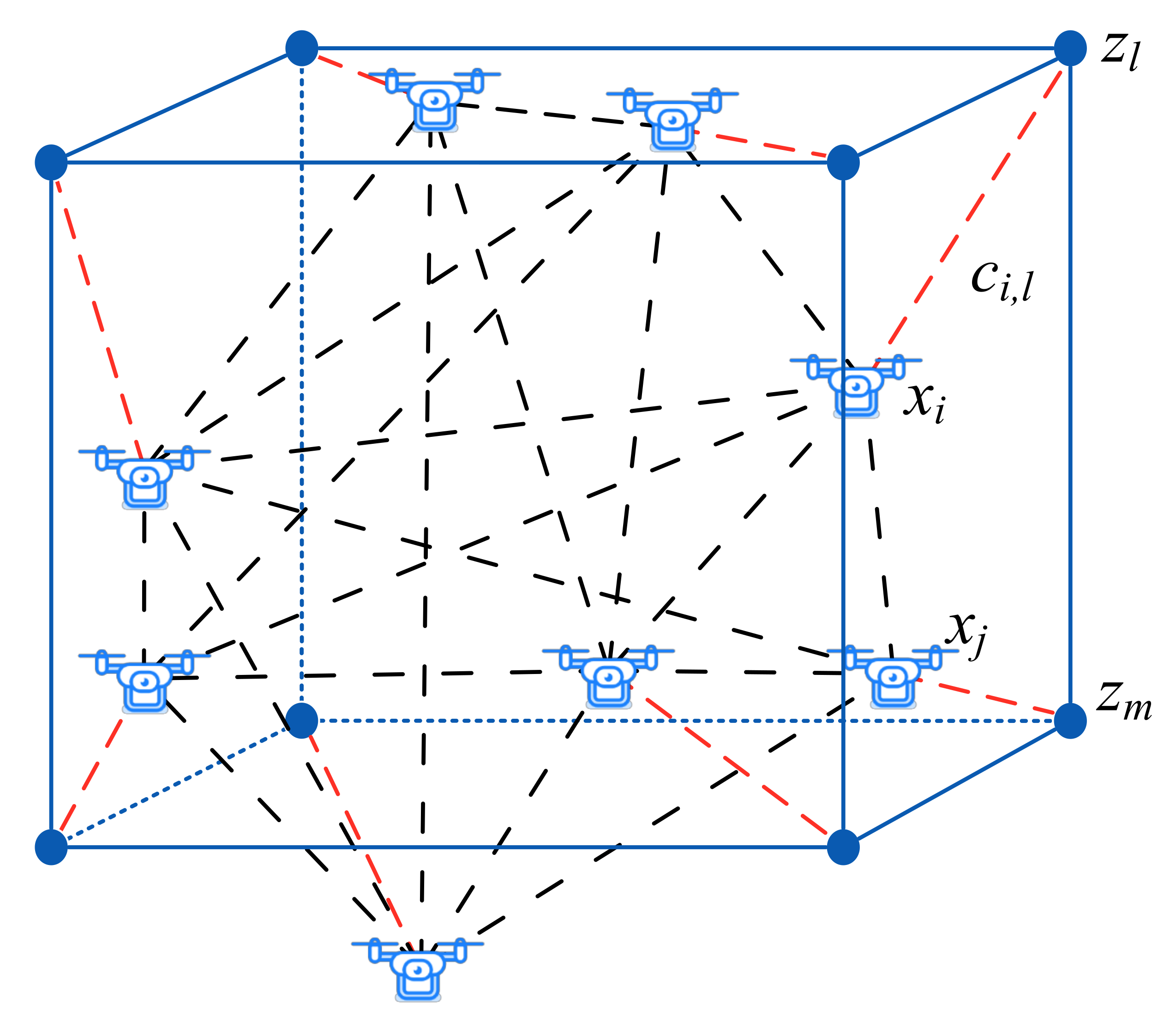
• From a global system perspective, a system optimization model for topology shaping of UAV swarm in 3D space is developed without relying on any external localization information, in which the topology shaping and global energy consumption minimization are considered.
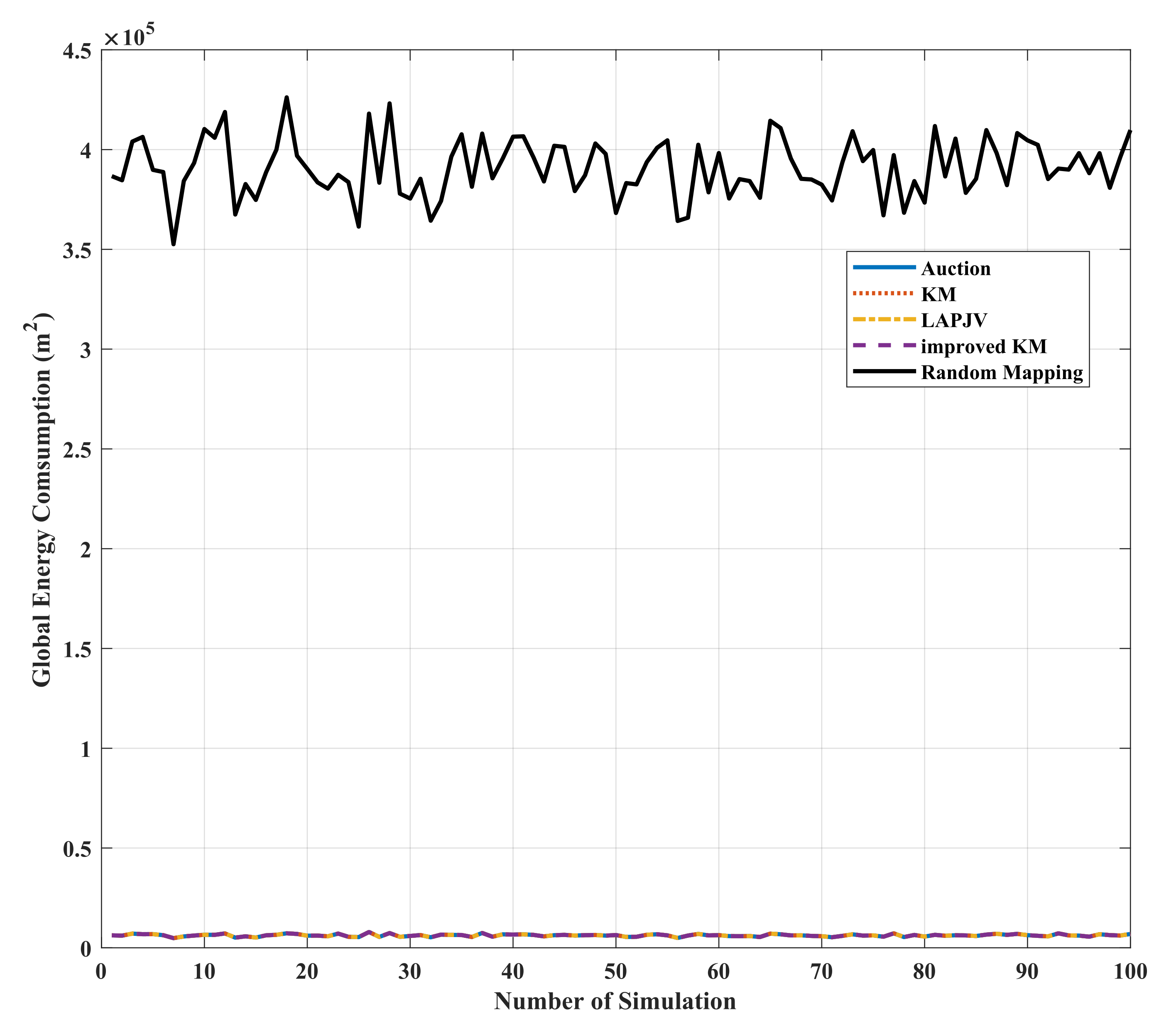
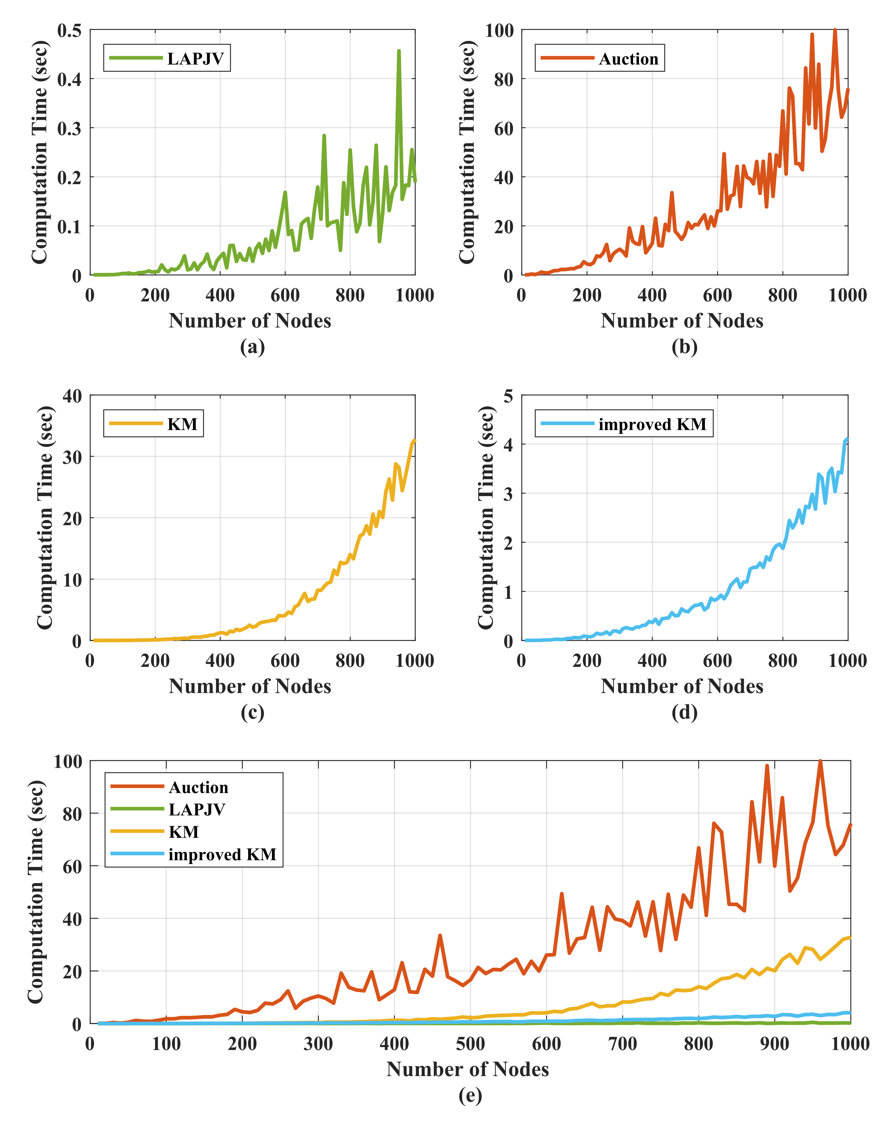
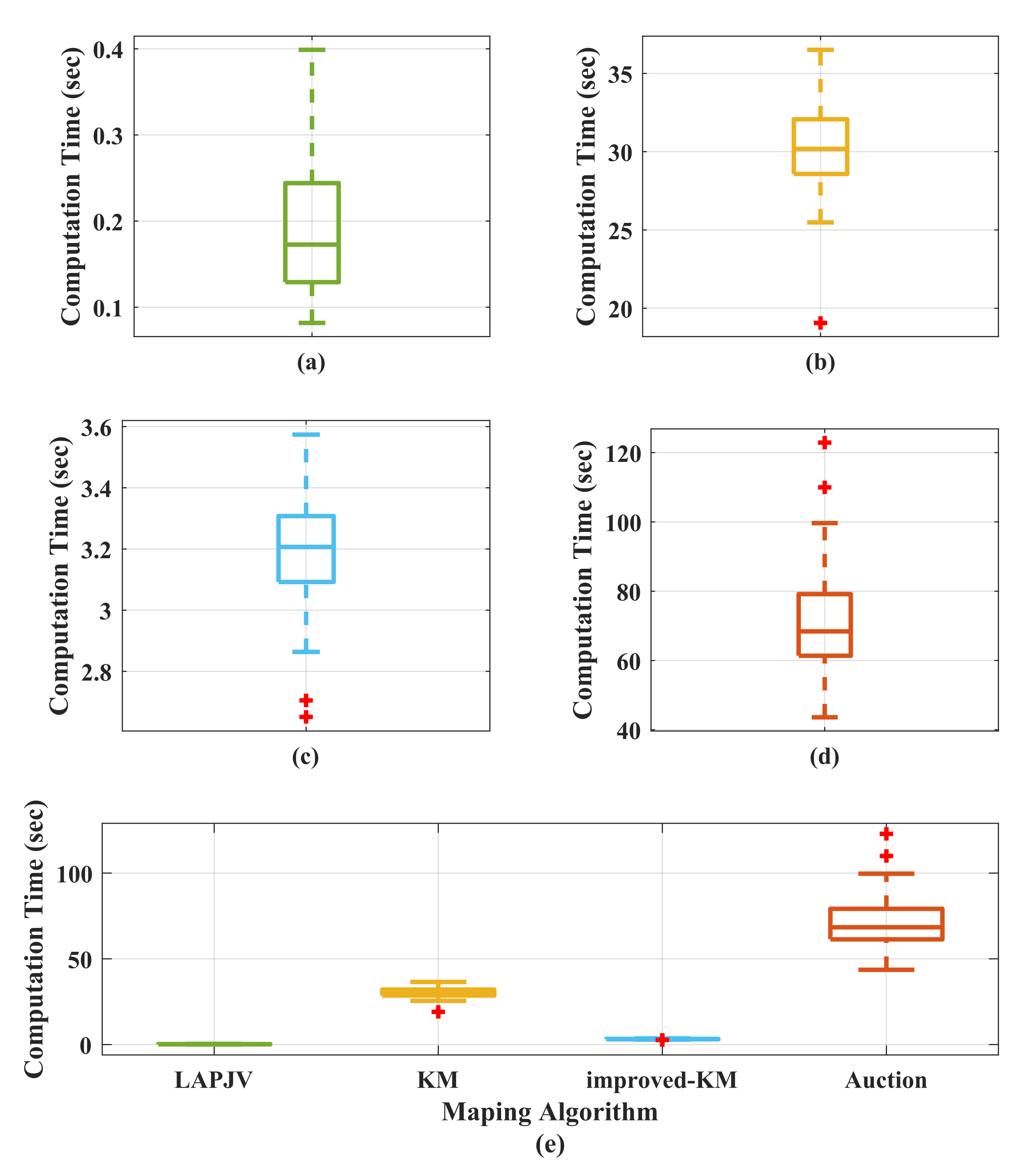
• Under the framework of the topology shaping optimization model, the topology shaping problem is transformed into a problem of relative coordinate mapping. The topology shaping with minimum global energy consumption is achieved by obtaining the optimal mapping relationship of the relative coordinates. The LAPJV algorithm is employed to solve this optimization model. The simulation results have demonstrated the effectiveness of this algorithm. The LAPJV algorithm significantly reduces the computational complexity by an average of $94\%$ in the case of 1000 UAV nodes while achieving the same minimum global energy consumption as other algorithms.

The rest of this paper is organized as follows. In Section 2, the system model of topology shaping for the UAV swarm system is presented. In Section 3, the initial and target topology coordinate systems are constructed based on the inter-distance of nodes without relying on any external localization information. In Section 4, the corresponding relationship of the UAVs from the initial topology to the target topology is derived through optimal coordinate mapping. Numerical simulations and results are shown in Section 5, followed by conclusions and discussions presented in Section 6.

2. System Model

A UAV swarm (target topology shape is a cube denoted by the blue dots) consisting of N homogeneous nodes in a 3D Euclidean space is shown in Figure 1. All UAV nodes can obtain the relative distance between each other without external localization information.

The coordinate system of the initial topology is constructed based on the inter-distance between nodes. Given that the coordinates of node i in the initial topology are ${\mathbf{x}}_i={[a_i,b_i,c_i]}^T\in {\mathbb{R}}^{3\times 1},i=1,2,\dots ,N$, and $\mathbf{X}={\left[{\mathbf{x}}_i^T\right]}_{N\times 1}={[{\mathbf{x}}_1,{\mathbf{x}}_2,{\mathbf{x}}_3,\dots ,{\mathbf{x}}_N]}^T\in {\mathbb{R}}^{N\times 3}$ denotes the coordinate matrix of initial topology. The distance between node i and j in the initial topology is denoted as ${\delta }_{ij}$, where

$$\begin{array}{cc}\hfill {\delta }_{ij}& =∥{\mathbf{x}}_i-{\mathbf{x}}_j∥\hfill \\ \hfill & =\sqrt{{\left(a_i-a_j\right)}^2+{\left(b_i-b_j\right)}^2+{\left(c_i-c_j\right)}^2},\hfill \end{array}$$

(1)

and $∥.∥$ denotes the Euclidean norm.

The coordinate system of target topology is constructed based on the inter-distance derived from the topology shape. Assuming that the coordinates of position l in the target topology are ${\mathbf{z}}_l={[a_l,b_l,c_l]}^T\in {\mathbb{R}}^{3\times 1},l=1,2,\dots ,N$, and $\mathbf{Z}={\left[{\mathbf{z}}_l^T\right]}_{N\times 1}={[{\mathbf{z}}_1,{\mathbf{z}}_2,{\mathbf{z}}_3,\dots ,{\mathbf{z}}_N]}^T$$\in {\mathbb{R}}^{N\times 3}$ denotes the coordinate matrix of target topology. The distance between $z_l$ and $z_m$ is denoted by

$$\begin{array}{c}\hfill d_{lm}=∥{\mathbf{z}}_l-{\mathbf{z}}_m∥.\end{array}$$

(2)

The energy consumption $c_{i,l}$ from node i to position $z_l$ in the topology forming process is assumed to be only related to the Euclidean distance between $x_i$ and $z_l$. Here, for the convenience of analysis, the coordinate origin and standard direction of the target coordinate system are assumed to be overlapped with the initial coordinate system, thus

$$\begin{array}{c}\hfill c_{i,l}=∥{\mathbf{x}}_i-{\mathbf{z}}_l∥.\end{array}$$

(3)

The energy consumption matrix, formed by the energy consumption of all possible mapping relationships, is denoted as

$$\begin{array}{cc}\hfill \mathbf{C}& ={\left[c_{i,l}\right]}_{N\times N}\hfill \\ \hfill & =\left[\begin{array}{ccccc}{c}_{1,1}& c_{1,2}& c_{1,3}& \cdots & c_{1,N}\\ c_{2,1}& c_{2,2}& c_{2,3}& \cdots & c_{2,N}\\ c_{3,1}& c_{3,2}& c_{3,3}& \cdots & c_{3,N}\\ ⋮& ⋮& ⋮& \ddots & ⋮\\ c_{N,1}& c_{N,2}& c_{N,3}& \cdots & c_{N,N}\end{array}\right].\hfill \end{array}$$

(4)

Let $M_{i,l}$ denote the mapping relationship between ${\mathbf{x}}_i$ and ${\mathbf{z}}_l$, $M_{i,l}=1$ means that the target position of ${\mathbf{x}}_i$ is ${\mathbf{z}}_l$, otherwise, $M_{i,l}=0$. $\mathbf{M}={\left[M_{i,l}\right]}_{N\times N}$ is the matrix of mapping relationship, which is expressed by

$$\begin{array}{cc}\hfill \mathbf{M}& ={\left[M_{i,l}\right]}_{N\times N}\hfill \\ \hfill & =\left[\begin{array}{ccccc}{M}_{1,1}& M_{1,2}& M_{1,3}& \cdots & M_{1,N}\\ M_{2,1}& M_{2,2}& M_{2,3}& \cdots & M_{2,N}\\ M_{3,1}& M_{3,2}& M_{3,3}& \cdots & M_{3,N}\\ ⋮& ⋮& ⋮& \ddots & ⋮\\ M_{N,1}& M_{N,2}& M_{N,3}& \cdots & M_{N,N}\end{array}\right].\hfill \end{array}$$

(5)

Only when $M_{i,l}=1$ will the $c_{i,l}$ in $\mathbf{C}$ be chosen to calculate the global energy consumption $C_g$ of topology forming. $C_g$ is expressed by

$$\begin{array}{c}\hfill C_g={∥\mathbf{C}{\mathbf{M}}^T∥}_1=\sum _{i=1}^N\sum _{l=1}^N{c}_{i,l}{M}_{i,l},\end{array}$$

(6)

where ${∥.∥}_1$ denotes the entrywise matrix norm [36].

In the following sections, according to the system model described above, the initial coordinate system is first established to determine the relative coordinates of the initial topology. Then, based on the target topology shape, the target coordinate system is established to obtain the coordinates of each target position. Finally, the optimal coordinate mapping relationship for topology shaping is derived with the minimized global energy consumption.

3. The Construction of Initial and Target Topology Coordinate Systems

The Multidimensional Scaling (MDS) algorithm is one of the dimensionality reduction techniques that transforms multidimensional data into a lower-dimensional space while retaining the inherent information [37,38,39]. The MDS algorithm uses distance as a criterion while maintaining the exact distances between the original points and the dimension-reduced points, thus can be used to establish the coordinate system according to the inter-distance information of nodes.

From Equation (1), it can be found that ${\delta }_{ij}={\delta }_{ji}$, ${\delta }_{ii}=0$, for all $i,j=1,2,\cdots ,N$. The distance matrix of initial topology is a symmetric matrix, which consists of ${\delta }_{ij}$ and expressed as

$$\begin{array}{c}\hfill \Delta ={\left[{\delta }_{ij}\right]}_{N\times N}=\left[\begin{array}{cccc}{\delta }_{11}& {\delta }_{12}& \cdots & {\delta }_{1N}\\ {\delta }_{21}& {\delta }_{22}& \cdots & {\delta }_{2N}\\ ⋮& ⋮& \ddots & ⋮\\ {\delta }_{N1}& {\delta }_{N2}& \cdots & {\delta }_{NN}\end{array}\right].\end{array}$$

(7)

According to $\Delta$, the square of distance ${\delta }_{ij}^2$ is calculated by

$$\begin{array}{cc}\hfill {\delta }_{ij}^2={∥{\mathbf{x}}_i-{\mathbf{x}}_j∥}^2& ={∥{\mathbf{x}}_i∥}^2+{∥{\mathbf{x}}_j∥}^2-2{\mathbf{x}}_i^T{\mathbf{x}}_j.\hfill \end{array}$$

(8)

In general, the geometric center of the swarm system is selected as the coordinate origin, which means

$$\begin{array}{c}\hfill \sum _i{\mathbf{x}}_i=0.\end{array}$$

(9)

Thus, ${\delta }_{ij}^2$ can be obtained as follows:

$$\begin{array}{cc}\hfill \sum _j{\delta }_{ij}^2& =N{∥{\mathbf{x}}_i∥}^2+\sum _j{∥{\mathbf{x}}_j∥}^2-2{\mathbf{x}}_i^T\sum _j{\mathbf{x}}_j\hfill \end{array}$$

$$\begin{array}{cc}\hfill & =N{∥{\mathbf{x}}_i∥}^2+\sum _j{∥{\mathbf{x}}_j∥}^2,\hfill \\ \hfill \sum _i{\delta }_{ij}^2& =N{∥{\mathbf{x}}_j∥}^2+\sum _i{∥{\mathbf{x}}_i∥}^2-2{\mathbf{x}}_j^T\sum _i{\mathbf{x}}_i\hfill \end{array}$$

(10)

$$\begin{array}{cc}\hfill & =N{∥{\mathbf{x}}_j∥}^2+\sum _i{∥{\mathbf{x}}_i∥}^2,\hfill \end{array}$$

(11)

$$\begin{array}{cc}\hfill \sum _{ij}{\delta }_{ij}^2& =N\sum _i{∥{\mathbf{x}}_i∥}^2+N\sum _j{∥{\mathbf{x}}_j∥}^2.\hfill \end{array}$$

(12)

Based on Equations (10)–(12), we obtain

$$\begin{array}{c}\hfill {∥{\mathbf{x}}_i∥}^2+{∥{\mathbf{x}}_j∥}^2=\frac{1}{N}\sum _i{\delta }_{ij}^2+\frac{1}{N}\sum _j{\delta }_{ij}^2-\frac{1}{N^2}\sum _{i,j}{\delta }_{ij}^2\end{array}$$

(13)

For the node relative coordinate ${\mathbf{x}}_i,i=1,2,3,\cdots ,N$, the initial relative coordinate matrix can be expressed by

$$\begin{array}{c}\hfill \mathbf{X}=\left[\begin{array}{c}{\mathbf{x}}_1^T\\ {\mathbf{x}}_2^T\\ ⋮\\ {\mathbf{x}}_N^T\end{array}\right].\end{array}$$

(14)

Defining a matrix

$$\begin{array}{c}\hfill \mathbf{Y}=\mathbf{X}{\mathbf{X}}^T,\end{array}$$

(15)

then for any $y_{ij},i,j=1,2,3\cdots ,N$, in $\mathbf{Y}$,

$$\begin{array}{c}\hfill y_{ij}={\mathbf{x}}_i^T{\mathbf{x}}_j.\end{array}$$

(16)

According to Equation (8), $y_{ij}$ can be derived by

$$\begin{array}{cc}\hfill y_{ij}& =-\frac{1}{2}\left({\delta }_{ij}^2-{∥{\mathbf{x}}_i∥}^2-{∥{\mathbf{x}}_j∥}^2\right).\hfill \end{array}$$

(17)

Combing Equations (13) and (17), $y_{ij}$ can be expressed by

$$\begin{array}{c}\hfill y_{ij}=-\frac{1}{2}\left[{\delta }_{ij}^2-\frac{1}{N}\sum _i{\delta }_{ij}^2-\frac{1}{N}\sum _j{\delta }_{ij}^2+\frac{1}{N^2}\sum _{i,j}{\delta }_{ij}^2\right].\end{array}$$

(18)

Based on Equation (18), the matrix $\mathbf{Y}$ can be obtained. By performing a eigen-decomposition [40], $\mathbf{Y}$ can be decomposed by

$$\begin{array}{c}\hfill \mathbf{Y}=\mathbf{U}\mathsf{\Lambda }{\mathbf{U}}^T=\mathbf{U}\sqrt{\mathsf{\Lambda }}{\left(\mathbf{U}\sqrt{\mathsf{\Lambda }}\right)}^T,\end{array}$$

(19)

where $\mathbf{U}$ is the matrix composed of the three eigenvectors of $\mathbf{Y}$, and $\mathsf{\Lambda }$ is the diagonal matrix composed of the three largest eigenvalues of $\mathbf{Y}$.

Finally, the initial relative coordinate matrix $\mathbf{X}$ can be obtained by

$$\begin{array}{c}\hfill \mathbf{X}=\mathbf{U}\sqrt{\mathsf{\Lambda }}.\end{array}$$

(20)

The solution procedure of $\mathbf{X}$ is shown in Algorithm 1.

Algorithm 1: Obtaining the coordinate matrix.

Input: Distance matrix $\Delta$, coordinate dimension $d=3$;

Output: Relative coordinate matrix $\mathbf{X}$;

1 Derive $y_{ij}$ by Equation (18) from $\Delta$;

2 Obtain Matrix $\mathbf{Y}$ from $y_{ij}$;

3 Eigen-decomposition of matrix $\mathbf{Y}$ and obtain the $eigenvalues$ and $eigenvectors$ of $\mathbf{Y}$;

4 Form the diagonal matrix $\Lambda$ by employ 3 largest $eigenvalues$;

5 Construct matrix $\mathbf{U}$ by $eigenvectors$;

6 Get $\mathbf{X}$ by Equation (20);

7 return$\mathbf{X}$;

The distance matrix $\mathbf{D}$ of target topology is a symmetric matrix, where $d_{lm}=d_{ml}$, $d_{ll}=0$, for all $l,m=1,2,\dots ,N$, and is expressed by

$$\begin{array}{c}\hfill \mathbf{D}={\left[d_{lm}\right]}_{N\times N}=\left[\begin{array}{cccc}{d}_{11}& d_{12}& \cdots & d_{1N}\\ d_{21}& d_{22}& \cdots & d_{2N}\\ ⋮& ⋮& \ddots & ⋮\\ d_{N1}& d_{N2}& \cdots & d_{NN}\end{array}\right],\end{array}$$

(21)

According to Algorithm 1, replacing the input distance matrix $\Delta$ with the distance matrix $\mathbf{D}$ of the target topology, the output of Algorithm 1 will be the target topology coordinate matrix $\mathbf{Z}$. The target coordinates of the target topology shape can be obtained from $\mathbf{Z}$.

4. The Optimal Coordinate Mapping from Initial Topology to Target Topology

The coordinates of initial and target topology have been derived based on Section 3, and the next step is to determine the target coordinates for each UAV.

The optimization model can be expressed by Equations (22)–(25).

$$\begin{array}{ccc}\hfill min& C_g=\sum _{i=1}^N\sum _{l=1}^N{c}_{i,l}{M}_{i,l},\hfill & \hfill \end{array}$$

(22)

$$\begin{array}{ccc}\hfill s.t.& \sum _{i=1}^N{M}_{i,l}=1,l=1,2,3,\cdots ,N,\hfill & \hfill \end{array}$$

(23)

$$\begin{array}{ccc}\hfill & \sum _{l=1}^N{M}_{i,l}=1,i=1,2,3,\cdots ,N,\hfill & \hfill \end{array}$$

(24)

$$\begin{array}{ccc}\hfill & M_{i,l}=0or1foralli,l=1,2,3,\cdots ,N.\hfill & \hfill \end{array}$$

(25)

Equation (22) is the objective function, which reflects the mapping relationship $M_{i,l}$ with the minimum sum of energy consumption $c_{i,l}$. Equations (23)–(25) are the constraint conditions of the mapping relationship, which mean only one position in $\mathbf{Z}$ can be selected for mapping with a node in $\mathbf{X}$. In this way, the topology shaping problem is transformed into a problem of determining the optimal mapping relationship between $\mathbf{X}$ and $\mathbf{Z}$ with minimal global energy consumption. The goal here is to find a mapping relation that minimizes global energy consumption, which has traditionally been formulated as a weighted bipartite graph problem and solved by employing the KM algorithm [24,26,27], the improved KM algorithm [41] or the Auction algorithm [20], even though the computational complexities of these algorithms are relatively high.

From the objective function Equation (22) and constraint conditions Equations (23)–(25), we can find that the optimal coordinate mapping can be formulated into a linear assignment problem (LAP), which is also known as a weighted bipartite matching problem.

In this paper, in order to obtain a topology shaping with minimal global energy consumption while reducing the computation time, the LAPJV algorithm [41,42,43,44] is adopted to solve the linear assignment problem (LAP).

The LAPJV algorithm, which is developed based on some common concepts with the KM algorithm, can significantly reduce the computation time of the whole algorithm by pre-processing the cost matrix and finding the shortest augmentation path. The computational complexity of the algorithm will be analyzed in Section 5.3.

The basic idea of the LAPJV algorithm is as follows:

• Select an unassigned node in the initial topology $\mathbf{X}$.
• Construct the residual (auxiliary, incremental) graph, ${\mathcal{G}}^{\prime }$ with costs $r_{ij}$.
• Find the shortest augmenting path via a modified Dijkstra algorithm (recall $r_{ij}\ge 0$).
• Augment the solution to improve the match, construct the auxiliary network and determine from unassigned row i to unassigned column j an alternating path of minimal total reduced cost.
• Update the dual variables so that CS conditions, i.e., $r_{ij}=u_i+v_j-c_{ij}=0$, hold.

The specific process of deriving optimal coordinate mapping through the LAPJV algorithm consists of two main steps, initialization and augmentation [44]. The input of the LAPJV algorithm is the cost matrix $\mathbf{C}$, the rows in $\mathbf{C}$ corresponding to the nodes in the initial topology, and the columns in $\mathbf{C}$ corresponding to the positions in the target topology. The element $c_{ij}$ in matrix $\mathbf{C}$ is the energy cost from node i to target position j. The process of the LAPJV algorithm is summarized in Algorithms 2 and 3, and the details are as follows.

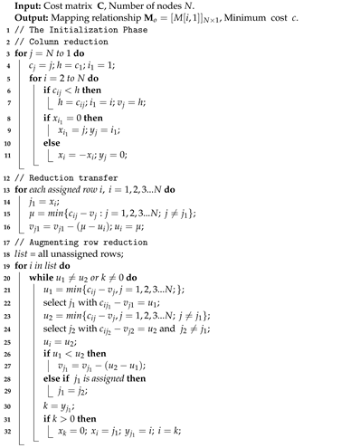
• The initialization phase including three sub-phases: column reduction, reduction transfer, augmenting row reduction.

  (a)

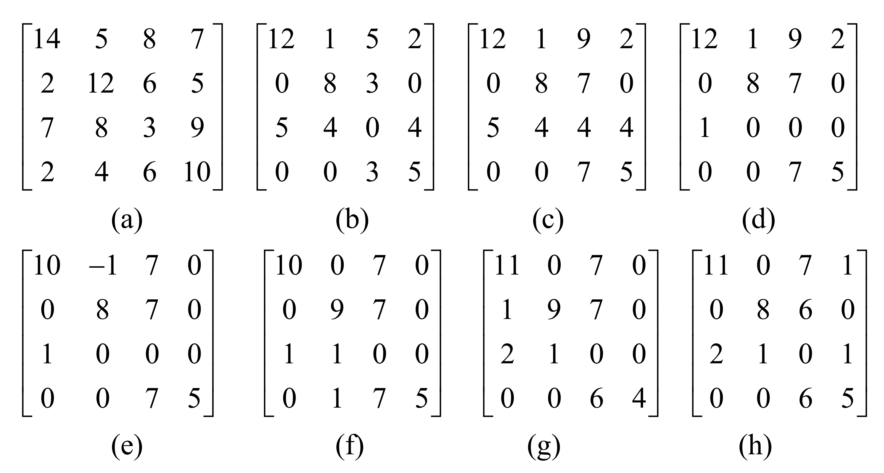
  Column reduction. Each element of a column subtracts a positive value. For the input cost matrix $\mathbf{C}$, from right to left, subtract the smallest value in the current column from each element in each column of the input matrix, as shown in Algorithm 2 (from line 3 to line 11). In this process, each column is assigned to a minimal row element, and some rows may not be assigned.

  (b)

  Reduction transfer, further reducing the unassigned rows. First, suppose the minimum value in the row i is $c_{ij}$, then perform the inverse column reduction, i.e., add $c_{ij}$ to all elements in column j. After that, subtract $c_{ij}$ from all elements in row i, as shown in Algorithm 2 (from line 13 to line 16).

  (c)

  Augmenting row reduction, trying to find a set of alternate paths. Starting from an unassigned row i, i.e., a node in initial topology, attempt to find the alternate path by first finding the current minimum value of $c_{ij}$ in row i, and then finding the second minimum value $c_{il}$, where $c_{il}\ge c_{ij}$. Next, reduce all elements of row i by $c_{il}$. If $c_{il}>c_{ij}$, the new $c_{ij}$ is negative. Assign i to column j with the reverse column reduction for column j. If column j has previously been assigned to row m, repeat this step from row m. This repeats until either row m is matched to an unassigned column, or it becomes impossible to transfer reduction to the selected row m. This process is shown in Algorithm 2 (from line 18 to line 32).

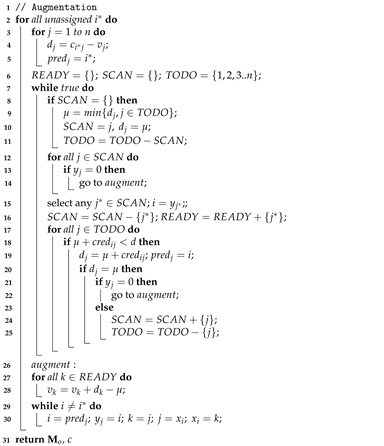
• The augmentation phase, which is the core of the algorithm to construct a bijective graph. For each unassigned row, the augmentation phase will find a shortest alternate path to the unassigned column through a modified Dijkstra’s algorithm. Starting with an unassigned row i, the search returns a shortest path to column j. If column j is assigned to row k, then add row k to the path. If the distances via row k to any given column are shorter, update these distances. After augmentation, all assignments correspond to the minimum value of each row in the cost matrix, which finally leads to the assignment with the lowest weight, i.e., the minimum global energy consumption. The assignment is the mapping relationship from the initial topology coordinates to the target topology coordinates. This process is shown in Algorithm 3.

Algorithm 2: Optimal Mapping Through Linear Assignment

For a more intuitive understanding of the LAPJV algorithm, an example of a step-by-step initialization process is provided. Consider a cost matrix C given in Figure 2a, which is a cost matrix of a four-node UAV swarm. The minimum element in the columns is 2, 4, 3, 5 respectively. The result of column reduction is shown in Figure 2b, in which each column reduces by its minimum element from right to left. Row 1 and column 4 are unassigned. Row 2 is assigned to column 1, row 3 is assigned to column 3, and row 4 is assigned to column 2. Reduction transfer is the following step of initialization. Consider row 3 of Figure 2b, we perform an inverse column reduction, which is to add the minimum element of row 3, i.e., 4 to column 3, the result of reduction transfer of row 3 is depicted in Figure 2c. Apply row reduction to row 3, and the result is illustrated as Figure 2d. The third step of the initialization phase is augmenting row reduction. Starting from unassigned row 1, the minimum element in row 1 is 2 (column 2) as depicted in Figure 2d, and the second minimum element is 2 (column 4). All the elements in row 1 are reduced by 2, and the result is depicted in Figure 2e. Perform inverse column reduction on column 2 and assign row 1 to column 2 and we obtain Figure 2f. Then the unassigned row is row 4. Perform the same augmenting row reduction procedure on row 4, and we obtain the result as shown in Figure 2g. The current unassigned row is row 2. Perform augmenting row reduction on row 2, and we obtain the result as depicted as Figure 2h. Then, the assignment is row 1 assigned to column 2, row 2 is assigned to column 4, row 3 is assigned to column 3, and row 4 is assigned to column 1. All rows are assigned after augmenting row reduction.

Algorithm 3: Augmentation Process of LAPJV

Then, according to the mapping relationships derived by Algorithms 2 and 3, the target position of each UAV can be obtained with minimum global energy consumption.

The LAPJV algorithm is a clever shortest augmenting path implementation of Hungarian which preprocesses the cost matrix by column reduction, reduction transfer, and reduction in unassigned rows, therefor the LAPJV algorithm does not need to perform the augmentation phase (Algorithm 3) too many times. From the examples given above, it is possible that the LAPJV algorithm has already completed the assignment in the initialization phase. Although the worst-case computational complexity of the LAPJV algorithm and the improved KM algorithm is $O\left(N^3\right)$ [45], in practice, the LAPJV algorithm takes less computation time in deriving the optimal mapping, thus the LAPJV algorithm is employed to solve the problem of optimal topology shaping.

The proposed topology shaping method is shown in Figure 3, and the specific process is as follows:

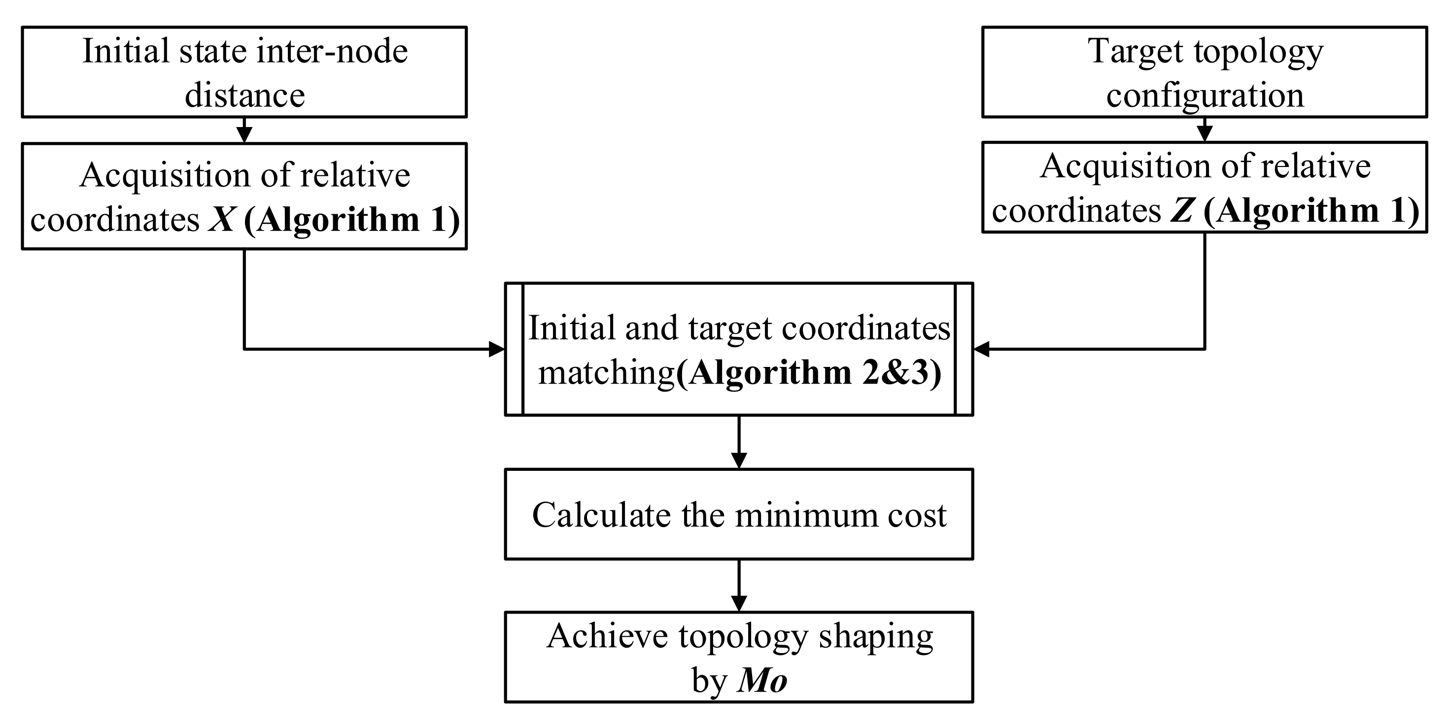
• Obtain the initial and target coordinates matrices $\mathbf{X}$ and $\mathbf{Z}$ by Algorithm 1.
• Obtain the optimal coordinate mapping relationship ${\mathbf{M}}_o$ by Algorithms 2 and 3.
• Achieve the topology shaping based on the optimal coordinate mapping relationship ${\mathbf{M}}_o$.

5. Numerical Results

In this section, the proposed topology shaping method’s validity is evaluated in different target topologies. In addition, its performance is also assessed in terms of energy consumption and computational complexity. All the simulation results are obtained from Matlab running on a personal computer (CPU 12th Gen Intel(R) Core(TM) i9-12900K, 128 GB RAM, Windows 11 Pro).

Two simulation scenarios are set to analyze the proposed topology shaping method. For the first scenario, the target topology shape is an aircraft with a length and wingspan of 350 m, and an aircraft height of 70 m. In total, 32 UAV nodes are randomly distributed in a 3D space of 1000 m × 1000 m × 1000 m. The specific simulation parameters are shown in

Table 1. Simulation parameters (aircraft shape).

$\mathrm{Parameter}$	$\mathrm{Value}$
Number of nodes	32
Spatial area	1000 m × 1000 m × 1000 m
Aircraft length	350 m
Aircraft wingspan	350 m
Aircraft height	70 m
Accuracy requirement	10${}^{-3}$

. For the second scenario, the target topology shape is a cube with a side length of 240 m. The number of nodes, spatial area and accuracy requirement are the same as in the first scenario. The corresponding simulation parameters are shown in

Table 2. Simulation parameters (cube shape).

$\mathrm{Parameter}$	$\mathrm{Value}$
Number of nodes	32
Spatial area	1000 m × 1000 m × 1000 m
Cube side length	240 m
Accuracy requirement	10${}^{-3}$

.

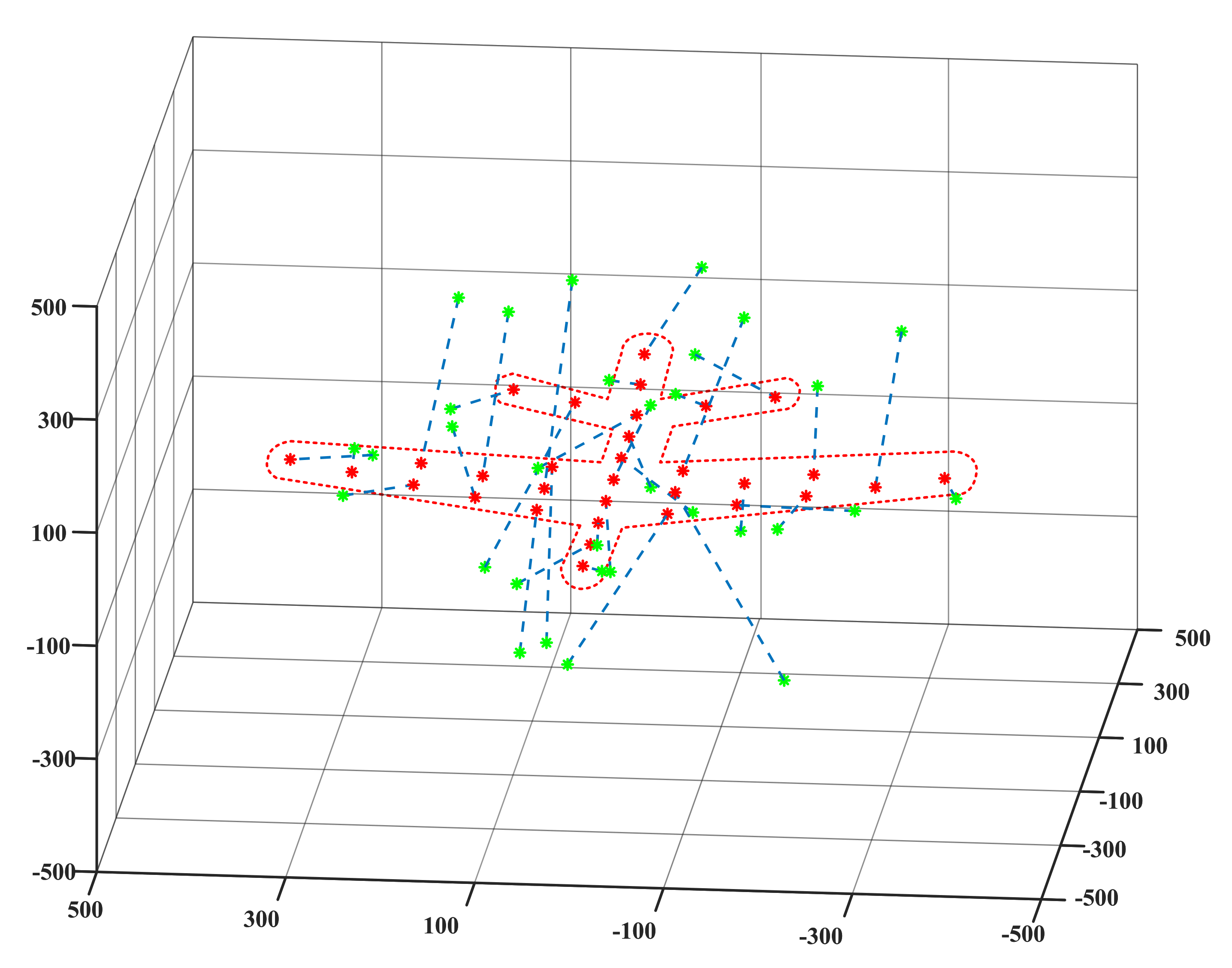
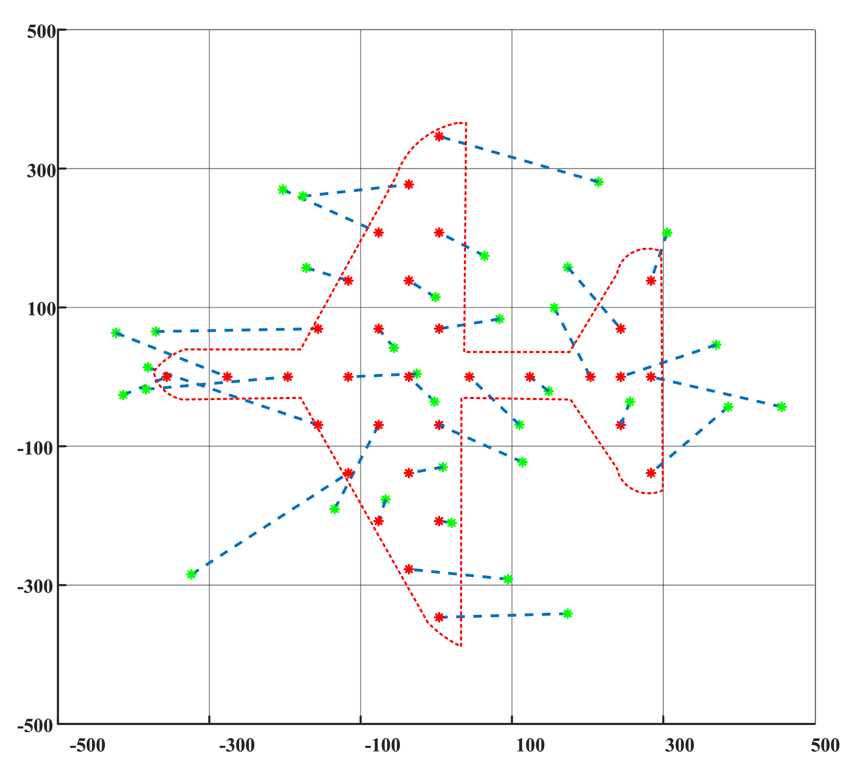
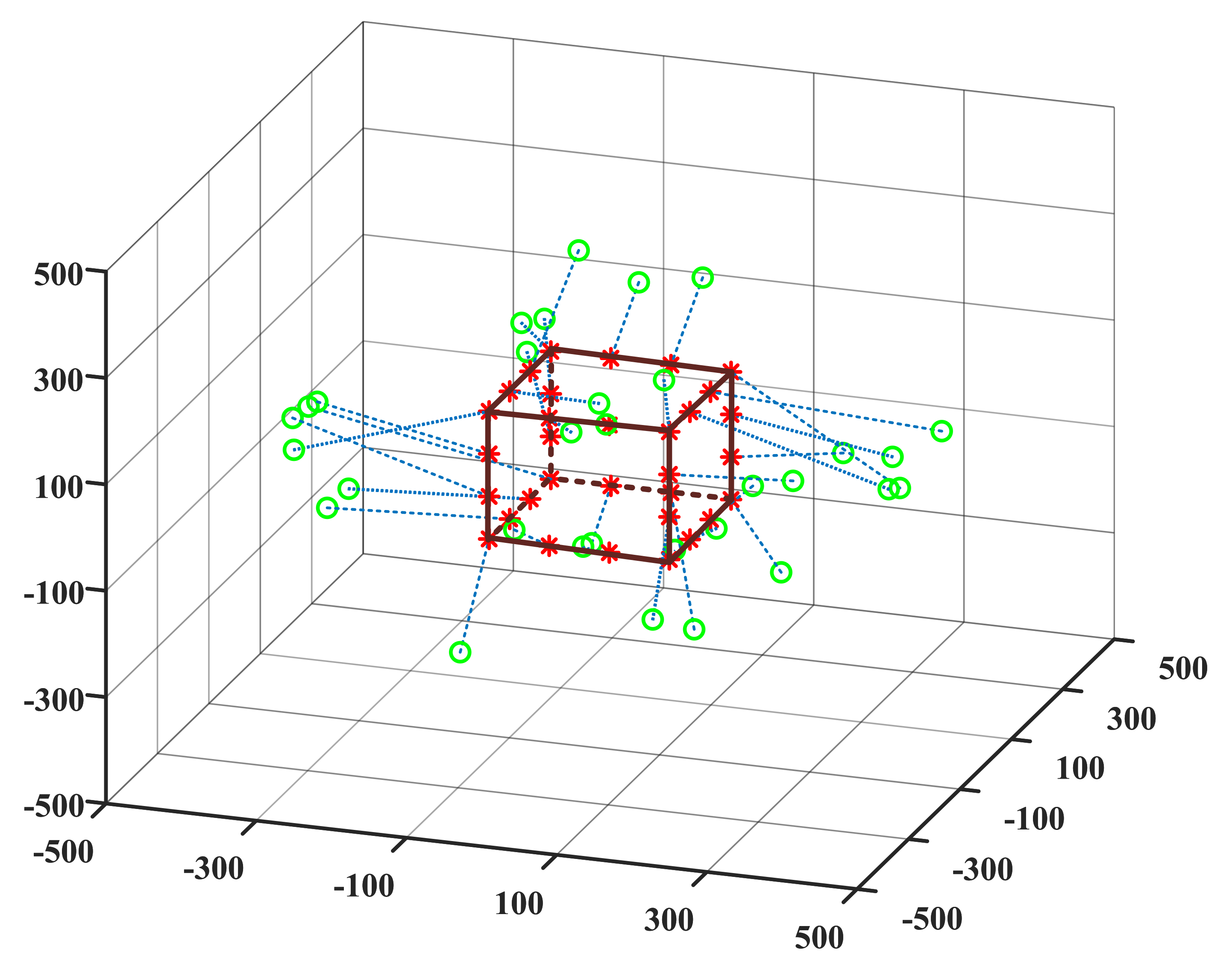
5.1. Validation of Proposed Topology Shaping Method

In order to analyze the validity of the proposed method, we performed the relevant simulations in both scenarios.

Simulation results of the first scenario are shown in Figure 4, Figure 5 and Figure 6, where the green asterisks represent the initial positions of nodes while the red asterisks represent the target positions, and the blue dashed lines denote the mapping relationship between them. The red dashed line is the outline of target topology. It can be seen that the desired topology shaping is successfully achieved based on the proposed method.

In the second simulation scenario, the target topology is a cube shape, and its topology shaping process is the same as in the first scenario. Simulation results are shown in Figure 7, where the green circles represent the initial positions of nodes while the red asterisks represent the target positions. The solid black line indicates the outline of target topology, and the blue dashed lines represent the mapping relationship between initial and target topology. It can be seen that the desired topology shaping is successfully achieved by the proposed method.

5.2. Global Energy Consumption

In order to analyze the global energy consumption, 100 sets of simulations are conducted. In each simulation, the initial topology is randomly distributed in the 3D space of 1000 m × 1000 m × 1000 m, and the target topology is an aircraft shape as shown in Table 1.

To evaluate the performance of proposed algorithm, the global energy consumption of the Auction algorithm, the KM algorithm, the improved KM algorithm and random mapping are compared. It is worth noting that the random mapping randomly selects a set of mapping relationships in each simulation. Simulation results are shown in Figure 8. From the simulation results, it can be seen that the average global energy consumption of the proposed method is reduced by about $98.4\%$ compared with that of the random mapping. On the other hand, the LAPJV algorithm can achieve the same global energy consumption compared with that of the KM algorithm, the improved KM algorithm, and the Auction algorithm.

5.3. Computational Complexity

In this subsection, the computational complexity of the proposed topology shaping method is analyzed and compared.

For a UAV swarm system consisting of N nodes, from Algorithm 2 we can see that the computational complexity of the column reduction process (from line 3 to line 11) is $O\left(5N^2\right)$. The computational complexity of the reduction transfer process (from line 13 to line 16) is $O\left(mN\right)$, in which m is the assigned row after column reduction. The computational complexity of the augmenting row reduction process is $O\left(R{N}^2\right)$, in which R is the range of the cost coefficients [42]. From Algorithm 3, we can find that the computational complexity of the augmentation phase is $O\left(N^3\right)$ [42].

The computational complexity of the Auction algorithm, the KM algorithm, and the improved KM algorithm is shown in

Table 3. Comparison of computation complexity.

$\mathrm{Algorithm}$	$\mathrm{Worst-Case\; Computation\; Complexity}$
Auction	$O\left(N^{2}logN\right)$ [46]
KM	$O\left(N^4\right)$ [41]
improved KM	$O\left(N^3\right)$ [45]

.

The computation time of the algorithm is a direct indicator of computational complexity. In order to compare the computational complexity of the LAPJV algorithm with the Auction algorithm, the KM algorithm, and the improved KM algorithm, we have conducted 100 sets of simulations for nodes varying from 10 to 1000. An extended comparison of the computation time is shown in Figure 9, in which (a), (b), (c), (d) are the curves of the average computation time of the LAPJV algorithm, the Auction algorithm, the KM algorithm, and the improved KM algorithm as the number of UAVs vary, respectively. As shown in Figure 9e, the LAPJV algorithm always achieves an extremely low computation time compared with the other three algorithms when the number of nodes varies from 10 to 1000. The average computation time of the LAPJV algorithm increases with the number of UAVs but is consistently below $0.5s$ for the case of no more than 1000 nodes. More specifically, the average computation time of the Auction algorithm has exceeded $1s$ in the case of 90 UAVs, the KM algorithm exceeds $1s$ in the case of 390 UAVs, and the improved KM algorithm exceeds $1s$ in the case of 640 UAVs.

In the case of 1000 nodes, 100 sets of simulations have been implemented to further investigate the proposed method, and the simulation results are shown in Figure 10. The average computation time of the LAPJV algorithm is 0.19 s, while the KM algorithm takes 30.32 s, the improved KM algorithm takes 3.20 s, and the Auction algorithm takes 71.99 s, which means that the LAPJV algorithm reduces the computation time by $99.37\%$ over the KM algorithm, $94.01\%$ over the improved KM algorithm, and $99.73\%$ over the Auction algorithm.

From the simulation results, we can see that the computation time of the LAPJV algorithm is much lower than that of the improved KM algorithm, the Auction algorithm, and the KM algorithm, which is due to the fact that the only a small percentage of nodes will perform the augmentation phases (computational complexity $O\left(N^3\right)$) after the initialization phase (computational complexity $O\left(N^2\right)$).

For better illustration, ${10}^4$ simulations have been conducted trying to identify the reason for the low computational complexity of the LAPJV algorithm. In the simulations, the number of UAVs is 1000. The assignment results and computation time of the initialization phase (including column reduction, reduction transfer, augmenting reduction) and the augmentation phase of the LAPJV algorithm are logged and analyzed. The statistics of assignments from the initial topology to the target topology are shown in Figure 11. From the simulation results, the average percentage of assigned UAVs in the initialization phase and the augmentation phase are $99.99831\%$ and $0.00169\%$, respectively.

That is to say, $99.99831\%$ of the nodes have been assigned in the initialization phase with a computational complexity of $O\left(N^2\right)$. According to Algorithm 3, only nodes that have not yet been assigned will be processed in the augmentation phase, which means that only $0.00169\%$ of the nodes will implement the augmentation phase with a computational complexity of $O\left(N^3\right)$). Thus, even though the worst-case computational complexity of the LAPJV algorithm is the same as the improved KM algorithm, which is $O\left(N^3\right)$, the average computational complexity of the LAPJV algorithm is much lower.

6. Conclusions and Future Work

The topology shaping method is the significant basis of functional topology construction in UAV swarm applications. In this paper, an LAPJV-based topology shaping method is proposed for the UAV swarm system. In this method, the mapping relationship from initial topology to target topology with minimum global energy consumption is fully considered. First, without relying on external localization information, the coordinates of the UAVs corresponding to the initial and target topology shape are derived by the MDS algorithm. Then, based on the linear assignment problem, the optimal mapping relationships with minimum global energy consumption are obtained through the LAPJV algorithm. Simulation results show that the proposed method can achieve optimal mapping with minimum global energy consumption for any target topology.

Moreover, although the worst-case computational complexities of the LAPJV algorithm are the same as the improved KM algorithm, the proposed LAPJV algorithm reduces computation time by over $94\%$ compared with the improved KM algorithm, the KM algorithm and the Auction algorithm in the case of 1000 UAV nodes. In addition, it does not rely on any external localization information, which is practical for swarming application scenarios in complex environments.

In our future work, the idea of parallel computing can be applied to the proposed topology shaping method to further reduce the computation time. Moreover, topology shaping can be achieved much faster by reducing the connectivity between UAVs to form a sparse distance matrix, which is a more practical model.

References

1. Lachow, I. The upside and downside of swarming drones. Bull. At. Sci. 2017, 73, 96–101. [Google Scholar] [CrossRef] [Green Version]
2. Skorobogatov, G.; Barrado, C.; Salamí, E. Multiple UAV systems: A survey. Unmanned Syst. 2020, 8, 149–169. [Google Scholar] [CrossRef]
3. Bekmezci, I.; Sahingoz, O.K.; Temel, Ş. Flying Ad-Hoc Networks (FANETs): A survey. Ad Hoc Netw. 2013, 11, 1254–1270. [Google Scholar] [CrossRef]
4. Haque, M.E.; Asikuzzaman, M.; Khan, I.U.; Ra, I.H.; Hossain, M.S.; Shah, S.B.H. Comparative Study of IoT-Based Topology Maintenance Protocol in a Wireless Sensor Network for Structural Health Monitoring. Remote Sens. 2020, 12, 2358. [Google Scholar] [CrossRef]
5. Liu, X.; Yin, J.; Zhang, S.; Ding, B.; Guo, S.; Wang, K. Range-Based Localization for Sparse 3-D Sensor Networks. IEEE Internet Things J. 2019, 6, 753–764. [Google Scholar] [CrossRef]
6. Brook, A.; Ben-Dor, E. Automatic Registration of Airborne and Spaceborne Images by Topology Map Matching with SURF Processor Algorithm. Remote Sens. 2011, 3, 65–82. [Google Scholar] [CrossRef] [Green Version]
7. Qiu, T.; Zhang, S.; Si, W.; Cao, Q.; Atiquzzaman, M. A 3D Topology Evolution Scheme with Self-Adaption for Industrial Internet of Things. IEEE Internet Things J. 2020, 8, 9473–9483. [Google Scholar] [CrossRef]
8. Aslan, M.F.; Durdu, A.; Sabanci, K.; Ropelewska, E.; Gültekin, S.S. A Comprehensive Survey of the Recent Studies with UAV for Precision Agriculture in Open Fields and Greenhouses. Appl. Sci. 2022, 12, 1047. [Google Scholar] [CrossRef]
9. Doherty, P.; Rudol, P. A UAV Search and Rescue Scenario with Human Body Detection and Geolocalization. In AI 2007: Advances in Artificial Intelligence; Orgun, M.A., Thornton, J., Eds.; Springer: Berlin/Heidelberg, Germany, 2007; pp. 1–13. [Google Scholar]
10. Shakhatreh, H.; Sawalmeh, A.H.; Al-Fuqaha, A.; Dou, Z.; Almaita, E.; Khalil, I.; Othman, N.S.; Khreishah, A.; Guizani, M. Unmanned aerial vehicles (UAVs): A survey on civil applications and key research challenges. IEEE Access 2019, 7, 48572–48634. [Google Scholar] [CrossRef]
11. Junwei, Z.; Jianjun, Z. Study on multi-UAV task clustering and task planning in cooperative reconnaissance. In Proceedings of the 2014 Sixth International Conference on Intelligent Human-Machine Systems and Cybernetics, Hangzhou, China, 26–27 August 2014; Volume 2, pp. 392–395. [Google Scholar]
12. Chen, H.X.; Nan, Y.; Yang, Y. Multi-UAV reconnaissance task assignment for heterogeneous targets based on modified symbiotic organisms search algorithm. Sensors 2019, 19, 734. [Google Scholar] [CrossRef] [Green Version]
13. He, X.; Yu, W.; Xu, H.; Lin, J.; Yang, X.; Lu, C.; Fu, X. Towards 3D deployment of UAV base stations in uneven terrain. In Proceedings of the 2018 27th International Conference on Computer Communication and Networks (ICCCN), Hangzhou, China, 30 July–2 August 2018; pp. 1–9. [Google Scholar]
14. Lu, J.; Wan, S.; Chen, X.; Chen, Z.; Fan, P.; Letaief, K.B. Beyond Empirical Models: Pattern Formation Driven Placement of UAV Base Stations. IEEE Trans. Wirel. Commun. 2018, 17, 3641–3655. [Google Scholar] [CrossRef]
15. Luo, D.; Xu, W.; Wu, S.; Ma, Y. UAV formation flight control and formation switch strategy. In Proceedings of the 2013 8th International Conference on Computer Science Education, Colombo, Sri Lanka, 26–28 April 2013; pp. 264–269. [Google Scholar] [CrossRef]
16. Nedjah, N.; de Macedo Mourelle, L. Swarm Intelligent Systems; Springer: Berlin, Germany, 2006; Volume 26, pp. 3–25. [Google Scholar]
17. Yang, Y.; Xiao, Y.; Li, T. A Survey of Autonomous Underwater Vehicle Formation: Performance, Formation Control, and Communication Capability. IEEE Commun. Surv. Tutor. 2021, 23, 815–841. [Google Scholar] [CrossRef]
18. Liu, X.; Liu, Y.; Chen, Y.; Hanzo, L. Trajectory design and power control for multi-UAV assisted wireless networks: A machine learning approach. IEEE Trans. Veh. Technol. 2019, 68, 7957–7969. [Google Scholar] [CrossRef] [Green Version]
19. Chung, S.J.; Paranjape, A.A.; Dames, P.; Shen, S.; Kumar, V. A survey on aerial swarm robotics. IEEE Trans. Robot. 2018, 34, 837–855. [Google Scholar] [CrossRef] [Green Version]
20. Morgan, D.; Subramanian, G.P.; Chung, S.J.; Hadaegh, F.Y. Swarm assignment and trajectory optimization using variable-swarm, distributed auction assignment and sequential convex programming. Int. J. Robot. Res. 2016, 35, 1261–1285. [Google Scholar] [CrossRef] [Green Version]
21. Brandão, A.S.; Sarcinelli-Filho, M. On the guidance of multiple uav using a centralized formation control scheme and delaunay triangulation. J. Intell. Robot. Syst. 2016, 84, 397–413. [Google Scholar] [CrossRef]
22. Abeywickrama, H.V.; Jayawickrama, B.A.; He, Y.; Dutkiewicz, E. Empirical Power Consumption Model for UAVs. In Proceedings of the 2018 IEEE 88th Vehicular Technology Conference (VTC-Fall), Chicago, IL USA, 27–30 August 2018; pp. 1–5. [Google Scholar]
23. Babazadeh, R.; Selmic, R. Distance-Based Multiagent Formation Control with Energy Constraints Using SDRE. IEEE Trans. Aerosp. Electron. Syst. 2019, 56, 41–56. [Google Scholar] [CrossRef]
24. Sui, Z.; Pu, Z.; Yi, J. Optimal UAVs formation transformation strategy based on task assignment and Particle Swarm Optimization. In Proceedings of the 2017 IEEE International Conference on Mechatronics and Automation (ICMA), Kagawa, Japan, 6–9 August 2017; pp. 1804–1809. [Google Scholar] [CrossRef]
25. Fabra, F.; Wubben, J.; Calafate, C.T.; Cano, J.C.; Manzoni, P. Efficient and coordinated vertical takeoff of UAV swarms. In Proceedings of the 2020 IEEE 91st Vehicular Technology Conference (VTC2020-Spring), Antwerp, Belgium, 25–28 May 2020; pp. 1–5. [Google Scholar] [CrossRef]
26. Wubben, J.; Aznar, P.; Fabra, F.; Calafate, C.T.; Cano, J.C.; Manzoni, P. Toward secure, efficient, and seamless reconfiguration of UAV swarm formations. In Proceedings of the 2020 IEEE/ACM 24th International Symposium on Distributed Simulation and Real Time Applications (DS-RT), Prague, Czech Republic, 14–16 September 2020; pp. 1–7. [Google Scholar] [CrossRef]
27. Wubben, J.; Cecilia, J.M.; Calafate, C.T.; Cano, J.C.; Manzoni, P. Evaluating the effectiveness of takeoff assignment strategies under irregular configurations. In Proceedings of the 2021 IEEE/ACM 25th International Symposium on Distributed Simulation and Real Time Applications (DS-RT), Valencia, Spain, 27–29 September 2021; pp. 1–7. [Google Scholar] [CrossRef]
28. Gravell, B.; Summers, T. Concurrent goal assignment and collision-free trajectory generation for multiple aerial robots. IFAC-PapersOnLine 2018, 51, 75–81. [Google Scholar] [CrossRef]
29. Azam, M.A.; Mittelmann, H.D.; Ragi, S. UAV Formation Shape Control via Decentralized Markov Decision Processes. Algorithms 2021, 14, 91. [Google Scholar] [CrossRef]
30. Fu, X.; Pan, J.; Wang, H.; Gao, X. A formation maintenance and reconstruction method of UAV swarm based on distributed control. Aerosp. Sci. Technol. 2020, 104, 105981. [Google Scholar] [CrossRef]
31. Duan, H.b.; Ma, G.j.; Luo, D.l. Optimal formation reconfiguration control of multiple UCAVs using improved particle swarm optimization. J. Bionic Eng. 2008, 5, 340–347. [Google Scholar] [CrossRef]
32. Zhang, X.; Duan, H.; Yang, C. Pigeon-Inspired optimization approach to multiple UAVs formation reconfiguration controller design. In Proceedings of the 2014 IEEE Chinese Guidance, Navigation and Control Conference, Yantai, China, 8–10 August 2014; pp. 2707–2712. [Google Scholar] [CrossRef]
33. Duan, H.; Luo, Q.; Shi, Y.; Ma, G. Hybrid Particle Swarm Optimization and Genetic Algorithm for Multi-UAV Formation Reconfiguration. IEEE Comput. Intell. Mag. 2013, 8, 16–27. [Google Scholar] [CrossRef]
34. Balamurugan, G.; Valarmathi, J.; Naidu, V.P.S. Survey on UAV navigation in GPS denied environments. In Proceedings of the 2016 International Conference on Signal Processing, Communication, Power and Embedded System (SCOPES), Paralakhemundi, India, 3–5 October 2016; pp. 198–204. [Google Scholar] [CrossRef]
35. Oh, D.; Lim, J.; Lee, J.K.; Baek, H. Airborne-Relay-based Algorithm for Locating Crashed UAVs in GPS-Denied Environments. In Proceedings of the 2019 IEEE 10th Annual Ubiquitous Computing, Electronics Mobile Communication Conference (UEMCON), New York, NY, USA, 10–12 October 2019; pp. 0877–0882. [Google Scholar] [CrossRef]
36. Abbe, E.; Fan, J.; Wang, K. An theory lp of PCA and spectral clustering. arXiv 2020, arXiv:2006.14062. [Google Scholar]
37. Torgerson, W.S. Multidimensional scaling: I. Theory and method. Psychometrika 1952, 17, 401–419. [Google Scholar] [CrossRef]
38. Tzeng, J.; Lu, H.H.S.; Li, W.H. Multidimensional scaling for large genomic data sets. BMC Bioinform. 2008, 9, 179. [Google Scholar] [CrossRef] [PubMed] [Green Version]
39. Saeed, N.; Nam, H.; Haq, M.I.U.; Muhammad Saqib, D.B. A survey on multidimensional scaling. ACM Comput. Surv. (CSUR) 2018, 51, 1–25. [Google Scholar] [CrossRef] [Green Version]
40. Wickelmaier, F. An introduction to MDS. Sound Qual. Res. Unit Aalb. Univ. Den. 2003, 46, 1–26. [Google Scholar]
41. Jonker, R.; Volgenant, T. Improving the Hungarian assignment algorithm. Oper. Res. Lett. 1986, 5, 171–175. [Google Scholar] [CrossRef]
42. Jonker, R.; Volgenant, A. A shortest augmenting path algorithm for dense and sparse linear assignment problems. Computing 1987, 38, 325–340. [Google Scholar] [CrossRef]
43. Dell’Amico, M.; Toth, P. Algorithms and codes for dense assignment problems: The state of the art. Discret. Appl. Math. 2000, 100, 17–48. [Google Scholar] [CrossRef] [Green Version]
44. Jones, W.; Chawdhary, A.; King, A. Optimising the Volgenant–Jonker algorithm for approximating graph edit distance. Pattern Recognit. Lett. 2017, 87, 47–54, Advances in Graph-based Pattern Recognition. [Google Scholar] [CrossRef] [Green Version]
45. Lawler, E.L. Combinatorial Optimization: Networks and Matroids; Courier Corporation: Chelmsford, MA, USA, 2001. [Google Scholar]
46. Schwartz, B. A computational analysis of the auction algorithm. Eur. J. Oper. Res. 1994, 74, 161–169. [Google Scholar] [CrossRef]
Figure 1. An example of topology mapping for UAV swarm.
Applsci 12 02631 g001
Figure 2. A step-by-step example of the initialization process. (a) Example cost matrix; (b) After column reduction; (c) After reduction transfer of row 3; (d) After row reduction to row 3; (e) After reduce 2 in row 1; (f) After inverse column reduction on column 2; (g) After augmenting row reduction on row 4; (h) After augmenting row reduction on row 2.
Applsci 12 02631 g002
Figure 3. Flow chart of the proposed topology shaping method.
Applsci 12 02631 g003
Figure 4. The side perspective of topology shaping in aircraft shape.
Applsci 12 02631 g004
Figure 5. The X–Y perspective of topology shaping in aircraft shape.
Applsci 12 02631 g005
Figure 6. The X–Z perspective of topology shaping in aircraft shape.
Applsci 12 02631 g006
Figure 7. The side perspective of topology shaping in cube shape.
Applsci 12 02631 g007
Figure 8. Global energy consumption comparison between the proposed method(LAPJV), the Auction algorithm, the KM algorithm, the improved KM algorithm and random mapping.
Applsci 12 02631 g008
Figure 9. Computation time comparison between LAPJV, Auction, KM and improved KM as nodes varies from 10 to 1000. (a) Average computation time of the LAPJV algorithm; (b) Average computation time of the KM algorithm; (c) Average computation time of the improved KM algorithm; (d) Average computation time of the Auction algorithm; (e) Average computation time comparison of the four algorithms in the same scale.
Applsci 12 02631 g009
Figure 10. Computation time statistics of the four algorithms in the case of 1000 nodes. (a) Computation time statistics for the LAPJV algorithm; (b) Computation time statistics for the KM algorithm; (c) Computation time statistics for the improved KM algorithm; (d) Computation time statistics for the Auction algorithm; (e) Computation time statistics comparison for the four algorithms in the same scale.
Applsci 12 02631 g010
Figure 11. The number of assignment statistics in the case of 1000 nodes. (a) Number of assignment statistics after column reduction; (b) Number of assignment statistics after reduction transfer; (c) Number of assignment statistics after augmenting reduction; (d) Number of assignment statistics after augmenting phase.
Applsci 12 02631 g011