Article

Geochemical Association Rules of Elements Mined Using Clustered Events of Spatial Autocorrelation: A Case Study in the Chahanwusu River Area, Qinghai Province, China

1
Key Laboratory of Metallogenic Prediction of Nonferrous Metals and Geological Environment Monitoring (Ministry of Education), Central South University, Changsha 410083, China
2
School of Geosciences and Info-Physics, Central South University, Changsha 410083, China
*
Author to whom correspondence should be addressed.
Appl. Sci. 2022, 12(4), 2247; https://doi.org/10.3390/app12042247
Submission received: 20 January 2022 / Revised: 17 February 2022 / Accepted: 19 February 2022 / Published: 21 February 2022
(This article belongs to the Topic Data Science and Knowledge Discovery)

Abstract

:
The spatial distribution of elements can be regarded as a numerical field of concentration values with a continuous spatial coverage. An active area of research is to discover geologically meaningful relationships among elements from their spatial distribution. To solve this problem, we proposed an association rule mining method based on clustered events of spatial autocorrelation and applied it to the polymetallic deposits of the Chahanwusu River area, Qinghai Province, China. The elemental data for stream sediments were first clustered into HH (high–high), LL (low–low), HL (high–low), and LH (low–high) groups by using local Moran’s I clustering map (LMIC). Then, the Apriori algorithm was used to mine the association rules among different elements in these clusters. More than 86% of the mined rule points are located within 1000 m of faults and near known ore occurrences and occur in the upper reaches of the stream and catchment areas. In addition, we found that the Middle Triassic granodiorite is enriched in sulfophile elements, e.g., Zn, Ag, and Cd, and the Early Permian granite quartz diorite (P1γδο) coexists with Cu and associated elements. Therefore, the proposed algorithm is an effective method for mining coexistence patterns of elements and provides an insight into their enrichment mechanisms.

1. Introduction

Spatial autocorrelation analysis focuses on the similarity of attributes, as well as spatial similarity between one geological entity and adjacent entities. The spatial distribution of concentrations of elements can be regarded as a numerical field with a continued spatial coverage, which can be characterized by using spatial autocorrelation among different elements. Korobova and Romanov (2009) stressed that the nonrandom characteristics and spatial structure of geochemical data depend on the concentration field [1]. Analysis of the concentration field includes comparison of samples to recognize anomalies and using the spatial correlation among elements to explain geochemical processes. Geological interactions between elements result in mutual influence and restriction. Therefore, it is necessary to consider spatial auto- and cross correlation in geochemical studies. The concentrations and spatial association of different elements are usually related to parent lithostrata. Therefore, it is of great significance to study the distribution, enrichment, and relationships among different elements to understand regional magmatism and ore-forming process [2].
Tobler (1970) proposed the first law of geography: everything is related to everything else, but near things are more related than distant things [3]. The measurement of spatial autocorrelation includes global and local indicators. Global indicators reveal the spatial pattern of the whole region and reflect global characteristics. In contrast, local indicators measure the relationship between each location and its neighbors to reveal more detailed local spatial patterns. Global metrics include Moran’s I [4] and Geary’s C [5]. Improvements in spatial theory and statistical tests have made Moran’s I and Geary’s C the most widely used global indicators [6,7,8]. Based on Moran’s I, Cliff and Ord (1981) also proposed a simple spatiotemporal autocorrelation indicator form, Is-t [8]. Getis and Ord (1992, 1995) proposed global G statistic and local G* statistic [9,10]. Anselin (1995) developed local indicators of spatial association (LISA), including local Moran’s I and local Geary’s C [11]. Boots and Okabe (2007) proposed the concept of local spatial statistical analysis (LoSSA) both as an integrative structure for existing methods and as a framework that facilitates the development of new local and global statistics [12]. Anselin (2019) extended the application of the local Geary’s C statistic to a multivariate context. According to the characteristics of experimental data, each local autocorrelation indicator has its advantages and disadvantages [13]. Spatial autocorrelation indicators have been used in the fields of environmental science, regional economy, identification of diseases and mortality, and detection of geochemical anomalies [14,15,16,17,18].
The spatial pattern of the concentration field is caused by different geological processes [19]. The concentration field reflects the migration and spatiotemporal distribution of various elements. Therefore, both the spatial characteristics of a single element and the spatial relationship among multiple elements need to be considered.
For a long time, the identification and evaluation of geochemical anomalies has been a key issue in the field of geochemical exploration [20,21,22]. A geochemical anomaly is the enrichment or dilution of elements. The enriched area often has high mineral resource potential [23,24]. Geologists use the spatial pattern to distinguish an anomaly from the background. For many years, various statistical methods, such as mean ± 2 × standard deviations [25], probability graphs [26], univariate analysis [27], multivariate analysis [28,29], logistic regression [30,31], weights of evidence [32,33,34], fractal/multifractal models [35,36,37], and geostatistics [38,39], have been used to identify geochemical anomalies. In recent years, machine learning methods have been used in geological prospecting. These methods include support vector machines [40,41], random forests [42,43], Bayesian networks [44,45,46], and deep autoencoder networks [47].
Some small ore deposits or occurrences are overlooked in actual mineral prospecting if the association rules among elements are not considered [19]. How to efficiently delineate the metallogenic target area has become one of the main objectives of geochemical exploration. Nguyen et al. (2014) found that local Moran’s I could better detect the spatial clustering of elements in stream sediments on a small spatial scale than classical statistics, and local G* is suitable for detecting high clusters on a large scale [48]. Wang et al. (2015) used geostatistics, as well as fractal and spatial autocorrelation methods, to study the spatial characteristics of geochemical data for stream sediments in southwest Fujian and concluded that the spatial autocorrelation method delineates the geochemical anomaly [49]. Ji et al. (2017) used local Moran’s I to analyze the spatial clustering and outliers of elemental concentrations and extracted geochemical anomalies [50]. Yu et al. (2021) proposed a local correlation coefficient based on spatial neighborhoods to characterize the global distribution of elements [16].
The mutual influence and interaction among different elements produce a spatial pattern [51,52]. The effects of regional geological and geochemical processes can be inferred from the spatial patterns in the concentration field. Therefore, exploring the association rules among different elements is of great significance for understanding geological processes. Association rule mining is one of the branch fields of data mining. The Apriori algorithm can uncover Boolean association rules between itemsets and has been widely used in spatial data mining [53,54,55,56]. The Apriori algorithm was proposed by Agrawal et al. (1993), who used it to mine association rules of sales data obtained from a large retailing company [57]. Liu and Zhou (2019) used the Apriori algorithm to derive the anomalies of elements for metallogenic prediction [58].
In this paper, we propose an association rule mining method to study the cross correlation of concentration fields based on clustered events of spatial autocorrelation. This method can be used to comprehensively understand the spatial distribution of geochemical concentrations and co-existing of elements. Moreover, we compared the advantages and limitations of bivariate spatial autocorrelation and association rule mining results and finally explored the relationship of specific geological features with the results of association rule mining.

2. Study Area and Data

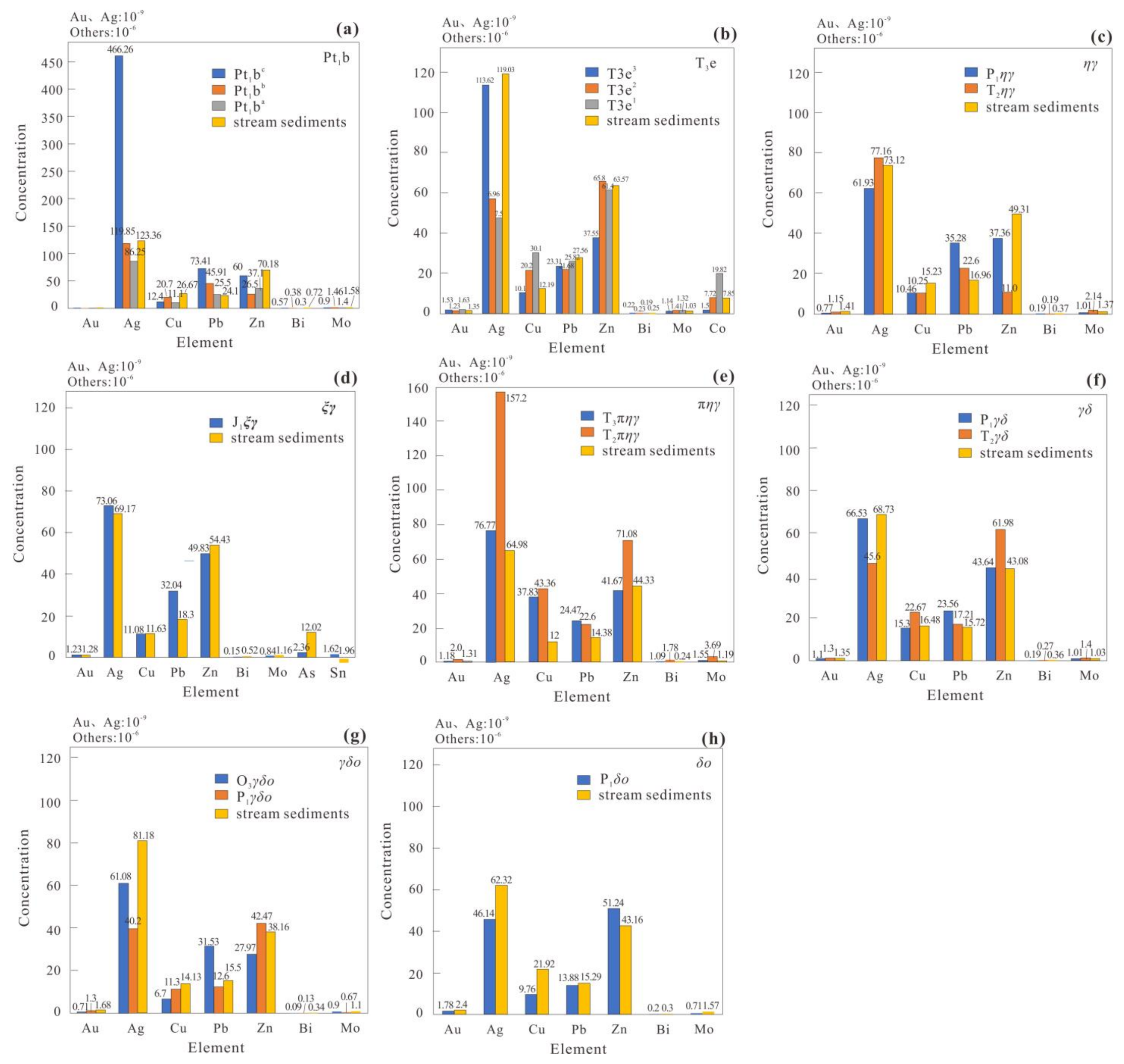
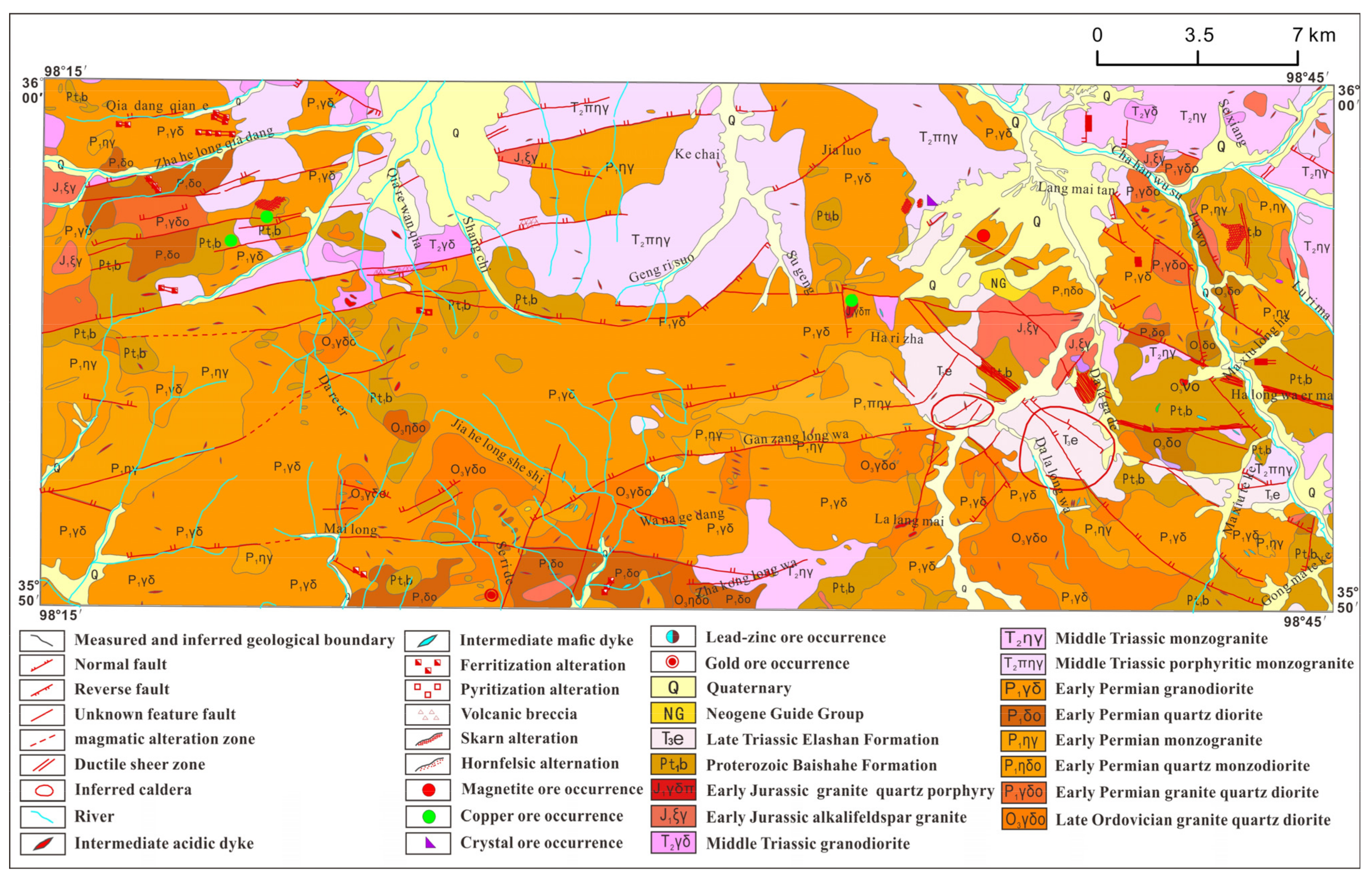
2.1. Geological Background

The Chahanwusu River area (98°15′ E–98°45′ E, 35°50′ N–36°00′ N) covers approximately 893 km2 in the eastern part of the East Kunlun tectonic belt in Dulan County in central Qinghai Province. The area is a polymetallic belt where one gold deposit, three copper deposits, one lead-zinc deposit two magnetite deposits, and one gemstone deposit have been found [59]. Figure 1 shows a geological map of the study area [43].
The main faults in the study area are EW-, NW-, and NE-trending and constitute the structural framework of the area. NW-trending faults are the most developed and control the distribution of strata and magmatic rocks. The sedimentary strata in the study area are undeveloped and dispersed. The outcropping strata, from old to new, are the Paleoproterozoic Baishahe Formation (Pt1b), the Late Triassic Elashan Formation (T3e), the Neogene Guide Group (NG), and Quaternary sediments (Q). Outcrops of intrusive rocks are widespread in the study area and are dominated by the Early Permian and the Middle Triassic intrusives.

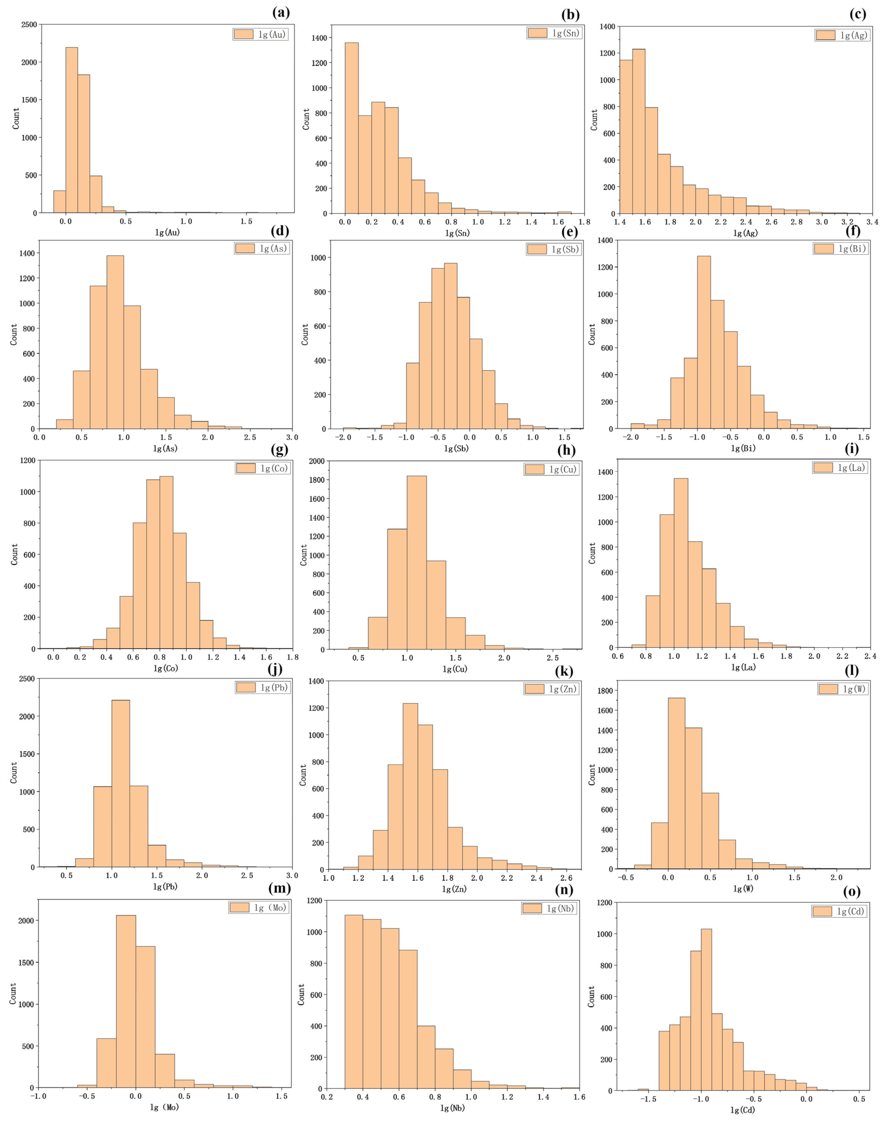
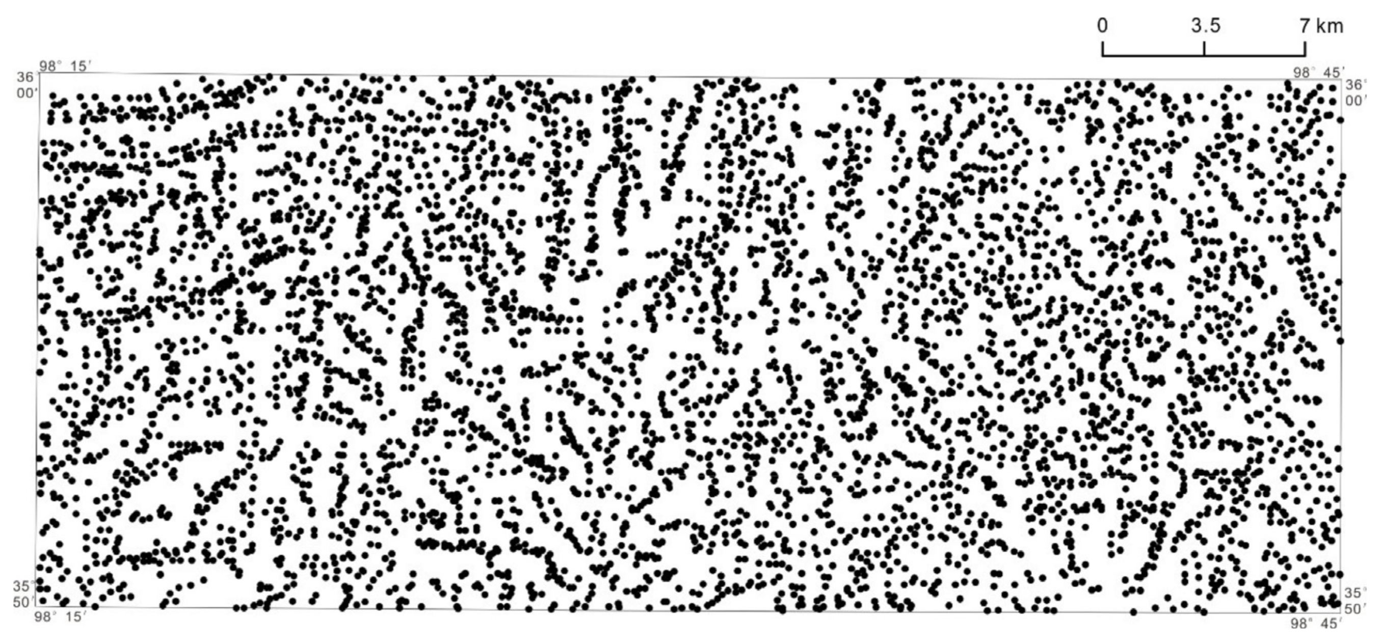
2.2. Geochemical Data

The datasets used in this study were geochemical analyses of 4959 stream sediment samples taken at a density of 5.55 points per 1 km2 by the Geological Survey Institute of Qinghai Province (Figure 2). The concentrations of 15 elements (Au, Sn, Ag, As, Sb, Bi, Co, Cu, La, Pb, Zn, W, Mo, Nb, and Cd) were measured in each sample. The samples were obtained through multi-pit combination sampling and were mainly collected from the debris materials of the bedrock composition in the catchment area, as well as medium- and coarse-grained sand in the stream sediments. The methods used to analyze the concentration of heavy metals include atomic emission spectrometry (AES) for Au, Ag, and Sn; atomic fluorescence spectrometry (AFS) for As, Sb, and Bi; atomic absorption spectrometry (AAS) for Cu, Pb, Zn, Co, and Ni; and polarography (POL) for W and Mo.
The elemental concentrations are summarized in Table 1. The coefficient of variation (CV) is expressed as the ratio of the standard deviation to the mean and is an important parameter that reflects the homogenization of element distribution. The elements with CV > 1, from largest to smallest, are Bi, W, Sb, As, Ag, Sn, Au, Cu, Pb, and Mo. Larger CV represents more inhomogeneous elemental concentrations. The higher the coefficient of variation, the greater the level of dispersion around the mean. We performed a logarithmic transformation on the 15 elements and plotted the log-frequency distribution histogram in the study area (Figure 3); therefore, we found that most elements tend to be lognormally distributed.
In addition, we compared the average concentrations of seven mineralized elements in the widely distributed bedrocks with those in the corresponding overlaying stream sediments (Figure 4). The element concentrations in the bedrocks and their corresponding overlaying stream sediments are very close; in particular, the two kinds of concentrations in the upper Triassic Elashan Formation almost coincide. The element concentrations show strong correlations between the bedrocks and their corresponding overlying stream sediments.

3. Methods

3.1. Spatial Autocorrelation

3.1.1. Univariate Spatial Autocorrelation

Spatial autocorrelation indicates the extent to which one attribute of a feature is related to nearby features [60]. Spatial autocorrelation indicators are the sum of the cross product of a similarity matrix, c i j , and a spatial similarity matrix, w i j , and include global (Equation (1)) and local (Equation (2)) metric indicators [11]. In general form, they are written as:
Γ g = i = 1 n j = 1 n c i j w i j
Γ i = j = 1 n c i j w i j
where n is the total number of observations, c i j is the self-similarity matrix, and w i j is the spatially weighted matrix.
Global indicators give the degree of spatial association for a single value, and local indicators assess the extent to which observations of similar and dissimilar values are clustered for each location [11]. Different measures of similarity yield different indices for spatial association [11]. For example, using c i j = x i x ¯ x j x ¯ yields a Moran-like indicator, setting c i j = x i x j 2 yields a Geary-like indicator, and setting c i j = x i x j yields a Getis–Ord-like indicator. The corresponding spatial autocorrelation indicators are global Moran’s I [4,6,7,8], Geary’s C [5,6,8], and Getis–Ord’s G [9], respectively. A global spatial autocorrelation indicator can only reflect the overall spatial trend and autocorrelation of the geographical entity or phenomenon. However, local spatial autocorrelation indicators measure the correlation among various locations and their neighbors to reveal more detailed local spatial patterns. These indicators include local Moran’s I [11], Geary’s C [11], and Getis–Ord’s G [9]. The calculation method of univariate global and local spatial autocorrelation statistics is shown in Table 2.

3.1.2. Multivariate Spatial Cross Correlation

Spatial cross correlation indicates the extent to which the multiple attributes of a feature are related to nearby features. The exploration of multivariate spatial cross correlation is a core functionality of current exploratory data analysis (EDA), knowledge discovery, and data mining tools [61]. Anselin et al. (2002) proposed bivariate global (Equation (3)) and local (Equation (4)) Moran’s I to quantify bivariate spatial cross correlation [62]. They are calculated from:
I a b = n i n j n w i j a i a ¯ b j b ¯ i n j n w i j i n a i a ¯ 2
I a b i = n a i a ¯ i n a i a ¯ 2 j n w i j b j b ¯
where a i and b j are the observed values of variables a and b at positions i and j , respectively; n is the total number of observations; a ¯ and b ¯ are the mean values of the observations of variables a and b , respectively; and w i j is the spatial weighted matrix.
Anselin (2019) proposed using the univariate local Geary’s C to measure the squared distance in attribute space (i.e., along a line for the univariate case) between the values at a geographic location and its neighboring locations, which is summarized in the form of a weighted sum [13]. This indicator can be readily extended to a multivariate context. For example, consider two variables, p and q . The squared distance, d i j 2 , in two-dimensional attribute space between the values at observation i and its geographic neighbor, j , is:
d i j 2 = p i p j 2 + q i q j 2
The bivariate local Geary’s C can be defined as:
c a b i = 1 2 j w i j d i j 2 = 1 2 j w i j p i p j 2 + q i q j 2 = 1 2 [ j w i j p i p j 2 + j w i j q i q j 2 ] = 1 2 ( c a i + c b i )
where p i and p j are the observed values of variable a at positions i and j , respectively; q i and q j are the observed values of variable b at positions i and j , respectively; and w i j is the spatial weighted matrix.
Following standard practice in multivariate clustering analysis, these variables have been standardized such that the mean of the transformed variable is zero and its variance is one. Moreover, the concept of a local Geary’ C is additive in the attribute dimension. Therefore, a multivariate local Geary’s C can be defined as:
c t o t a l i = v = 1 k   c v i / k
where k represents k -dimensional attribute space, and c v i represents the univariate local Geary’s C of variable v .

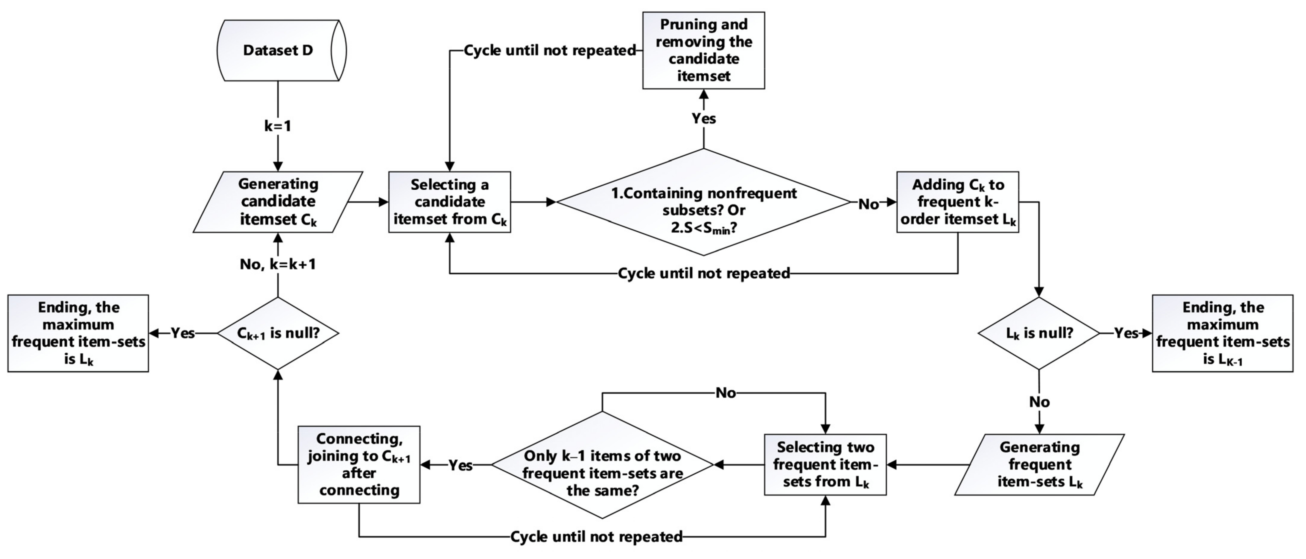
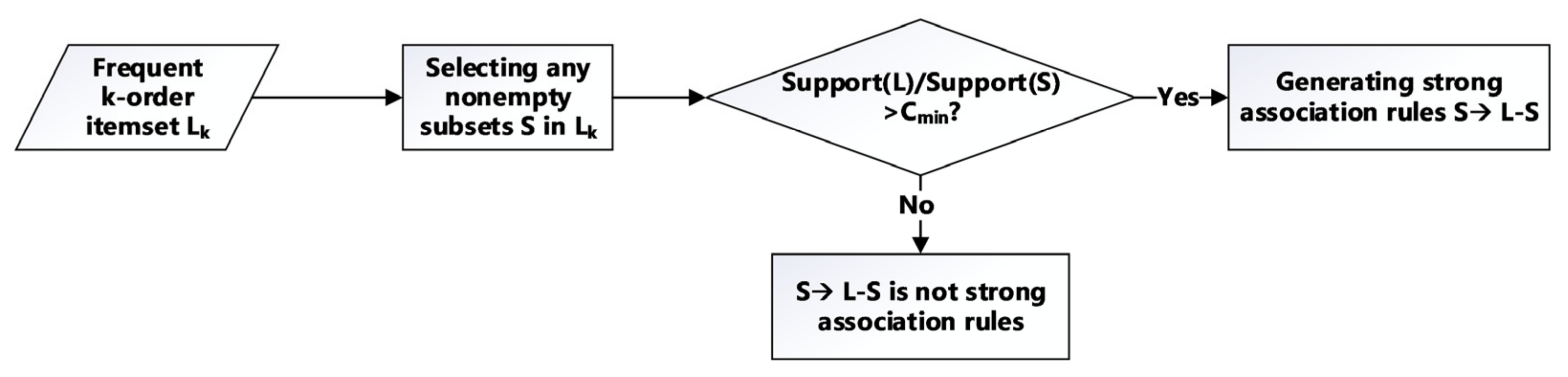
3.2. Association Rule Mining and Apriori Algorithm

Association rule mining is used to reveal the association among items in a dataset. We assume that   D = t 1 , t 2 , , t N is the event dataset, t k = i 1 , i 2 , , i K represents an event corresponding to a geochemical sample, and i k represents an item belonging to an aggregated event, t k . Itemset I = i 1 , i 2 , , i M is a specific item combination that contains M different items. For a subset, X in I , if X t k , then the event, t k , contains X . The goal of association rule mining is to find an implicit form of X Y , where X I , Y I , and X Y = . If the rule X Y exists, there are two key coefficients: the support degree, S, and confidence, C. The support degree,   S X Y = P X Y , represents the probability of co-occurrence of itemsets X and Y. The confidence,   C X Y = P Y | X = P X Y / P X , represents conditional probability of occurrence of itemset Y , given that itemset X has occurred. The itemsets that satisfy the minimum threshold (Smin) of support degree are so-called frequent itemsets, and those that satisfy both Smin and a minimum threshold of confidence (Cmin) are strong association rules.
The Apriori algorithm [57] can be decomposed into two main steps. The basic intuition is that any subset of a frequent itemset must be frequent. The first step is to generate frequent itemsets, as shown in Figure 5. The second step is to extract strong association rules based on frequent itemsets, as shown in Figure 6. The Apriori algorithm generates the candidate itemsets to be counted in a pass by using only the frequent itemsets in the previous pass. To improve the efficiency of frequent itemset extraction, the method utilizes a pruning strategy in order to compress the search space, that is, all non-empty subsets of frequent itemsets must also be frequent, and all parent sets of nonfrequent itemsets are nonfrequent.

4. Results and Discussion

4.1. Spatial Autocorrelation of Elements

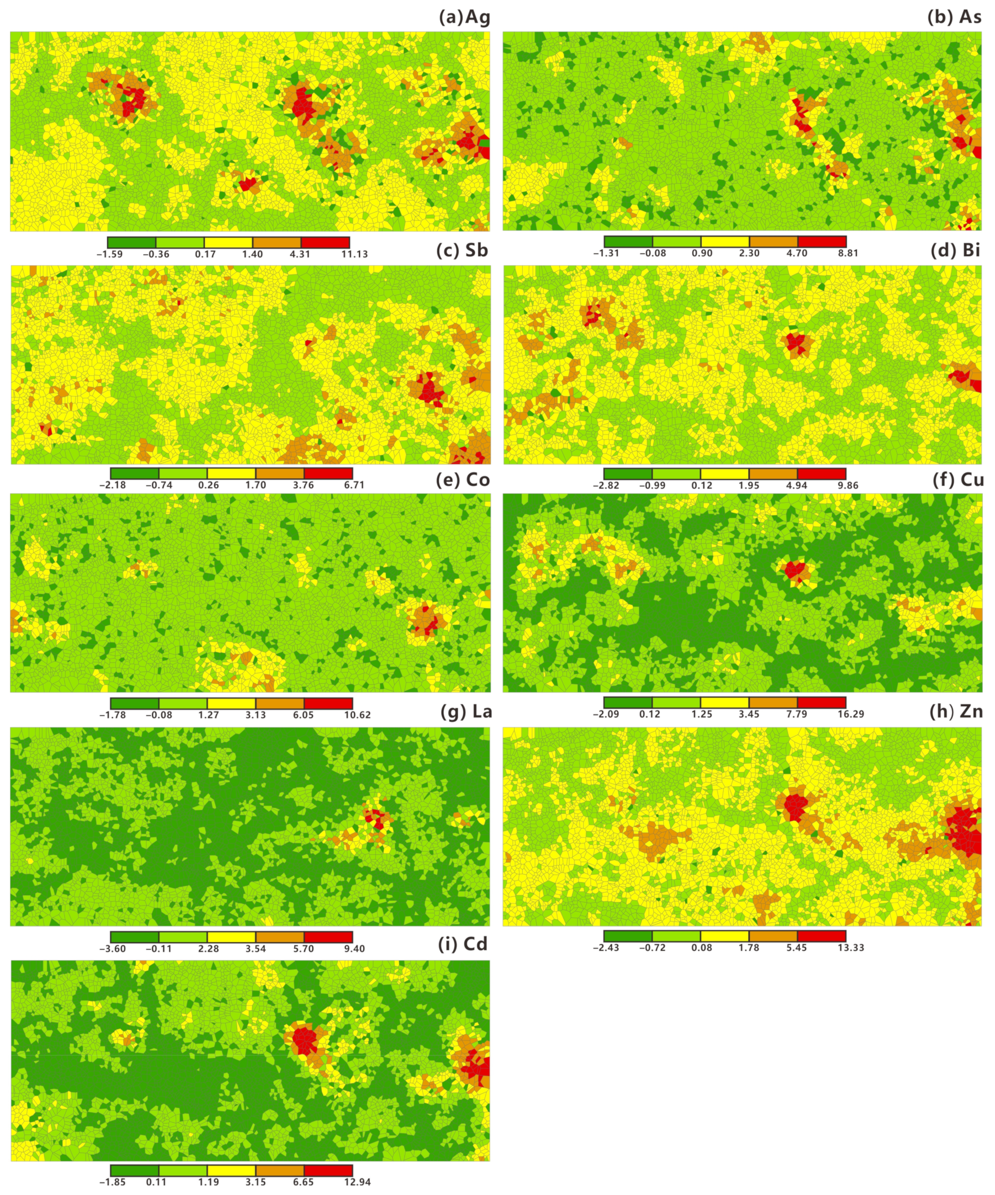
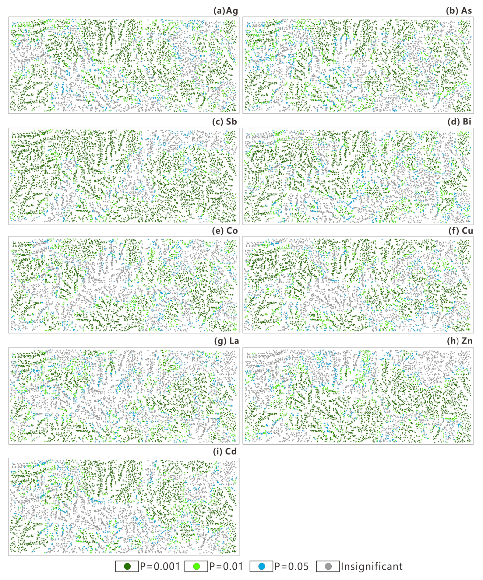
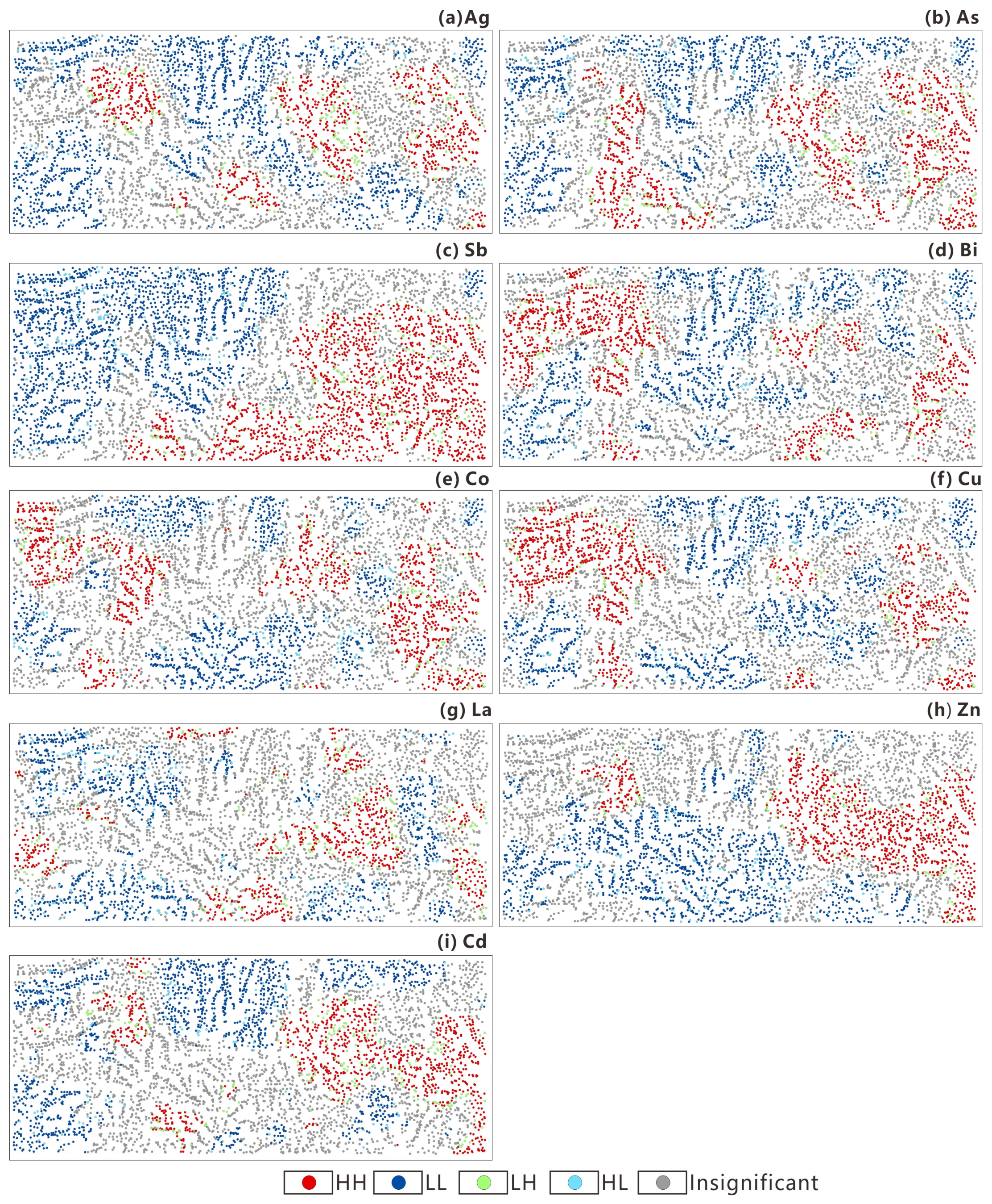
4.1.1. Univariate Spatial Autocorrelation of Individual Elements

We calculated the spatial autocorrelation and cross-correlation indicators of each element using open-source software packages Geoda (http://geodacenter.github.io, accessed on 28 May 2021) and spdep (https://github.com/r-spatial/spdep, accessed on 4 April 2021). Then, we applied the Z-score to test the significance of spatial autocorrelation and cross-correlation statistics. Because the global Moran’s I can be tested by normal or permutation tests [8], the Z-score was calculated by Monte Carlo simulation by randomly sampling 999 permutations. The global Moran’s I, global Geary’s C, and global Getis–Ord’s G for 15 elements passed the statistical significance test and were consistent with each other (Table 3). The global Moran’s I and Geary’s C are both suitable for characterizing the overall spatial pattern of an element; however, the global Getis–Ord’s G only indicates whether an element’s concentration exhibits a positive correlation (LL-clustered or HH-clustered) or is randomly distributed. It cannot be used to ascertain a negative correlation or compare the correlation between elements.
The global Getis–Ord’s G shows that all 15 elements have a positive correlation in the study area. The global Moran’s I and Geary’s C show that Au is randomly distributed, and the other 14 elements are positively correlated. The elements, ordered from high to low correlation, are Sb, Zn, Pb, Cu, Cd, As, Sn, Bi, Ag, Mo, Co, W, La, and Nb (Table 3). Except for Au, the global Moran’s I and Geary’s C are consistent with Getis–Ord’s G. According to the geological survey report, an Au deposit was found in the study area [59]. However, because of the low concentrations of Au in most sampling points of the study area, it would be easy to overlook the local clustering in the global spatial autocorrelation analysis.
We calculated the local Moran’s I of major elements in the study area and visualized the results via a Voronoi diagram (Figure 7). Anselin (1995) proposed a local indicator of spatial association (LISA) statistic that satisfies the following two requirements: (a) the LISA for each observation gives an indication of the extent of significant spatial clustering of similar values around that observation; and (b) the sum of LISAs for all observations is proportional to a global indicator of spatial association [11]. By calculating the local Moran’s I, I i , in each quadrant, this divides the concentrations of elements into five categories: insignificant, high–high (HH), low–low (LL), low–high (LH), or high–low (HL) clustering [11]. A local Moran’s I clustering map (LMIC) represents different types of association between the value at a given location and its spatial lag, i.e., the weighted average of the values in the surrounding locations. The LISA significance map is shown in Figure 8, in which we set p = 0.05. The local Moran’s I clustering map is shown in Figure 9. These results are consistent with the Moran’s I clustering results, which show that the HH and LL clustering in LMIC can reflect the spatial pattern of elements’ concentrations with a certain statistical significance. In addition, maps of local Moran’s I have natural transitions from strong to weak, which capture the local details and are consistent with the distributions of elements in nature.
Moreover, we also calculated indicators of the local Geary’s C and the local Getis–Ord’s G of all the elements in the study area. The HH- and LL-clustered values of the local Moran’s I and the local Geary’s C are similar; however, the local Getis–Ord’s G covers a broader space, especially for Sb, As, Cu, and Co. Compared with local Geary’s C and local Getis–Ord’s G, we can identify points with HH, LL, LH, and HL clustering with a precise meaning for each category from the local Moran’s I. Therefore, we chose the LMIC results to mine the association rules of various elements.

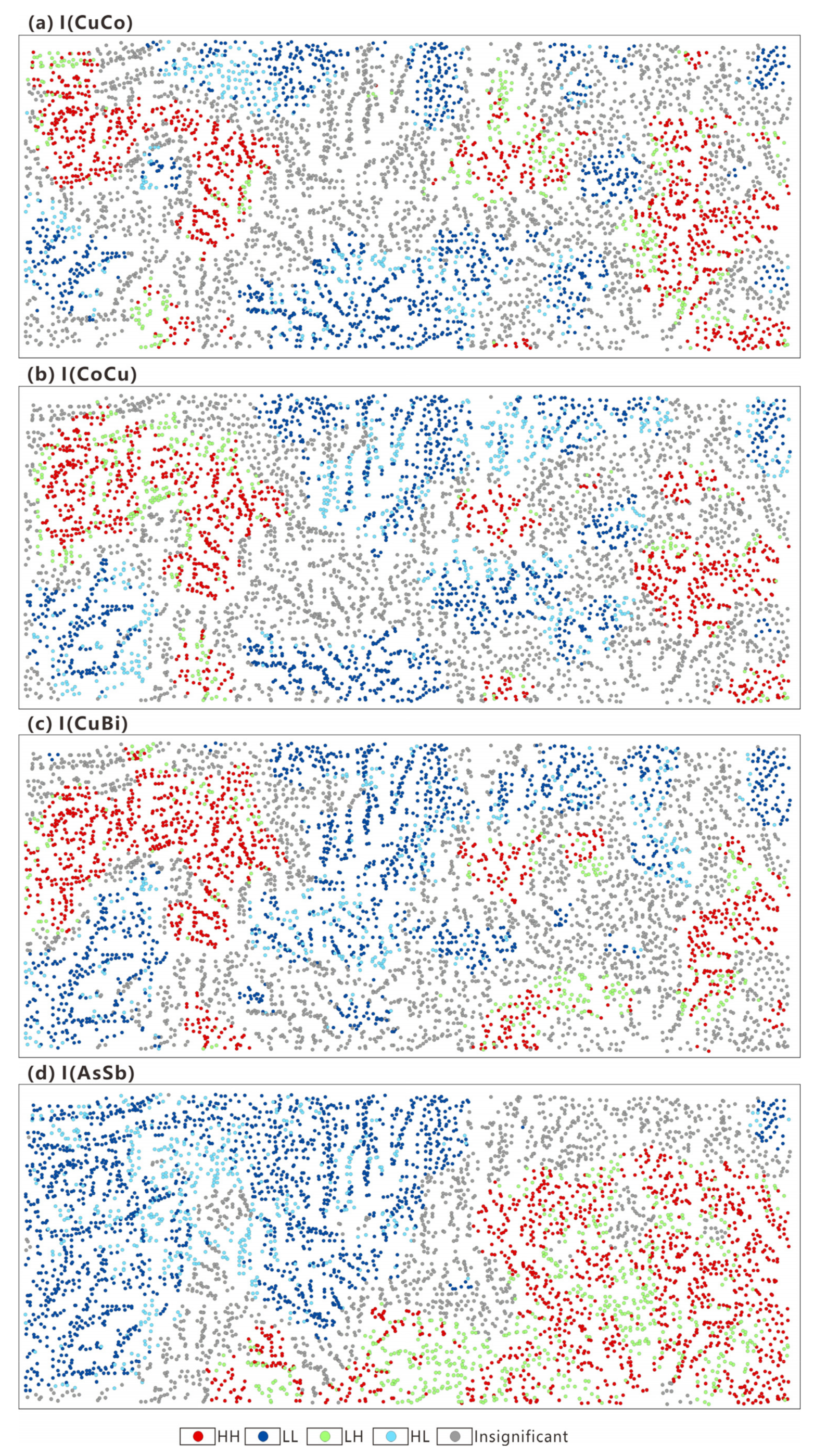
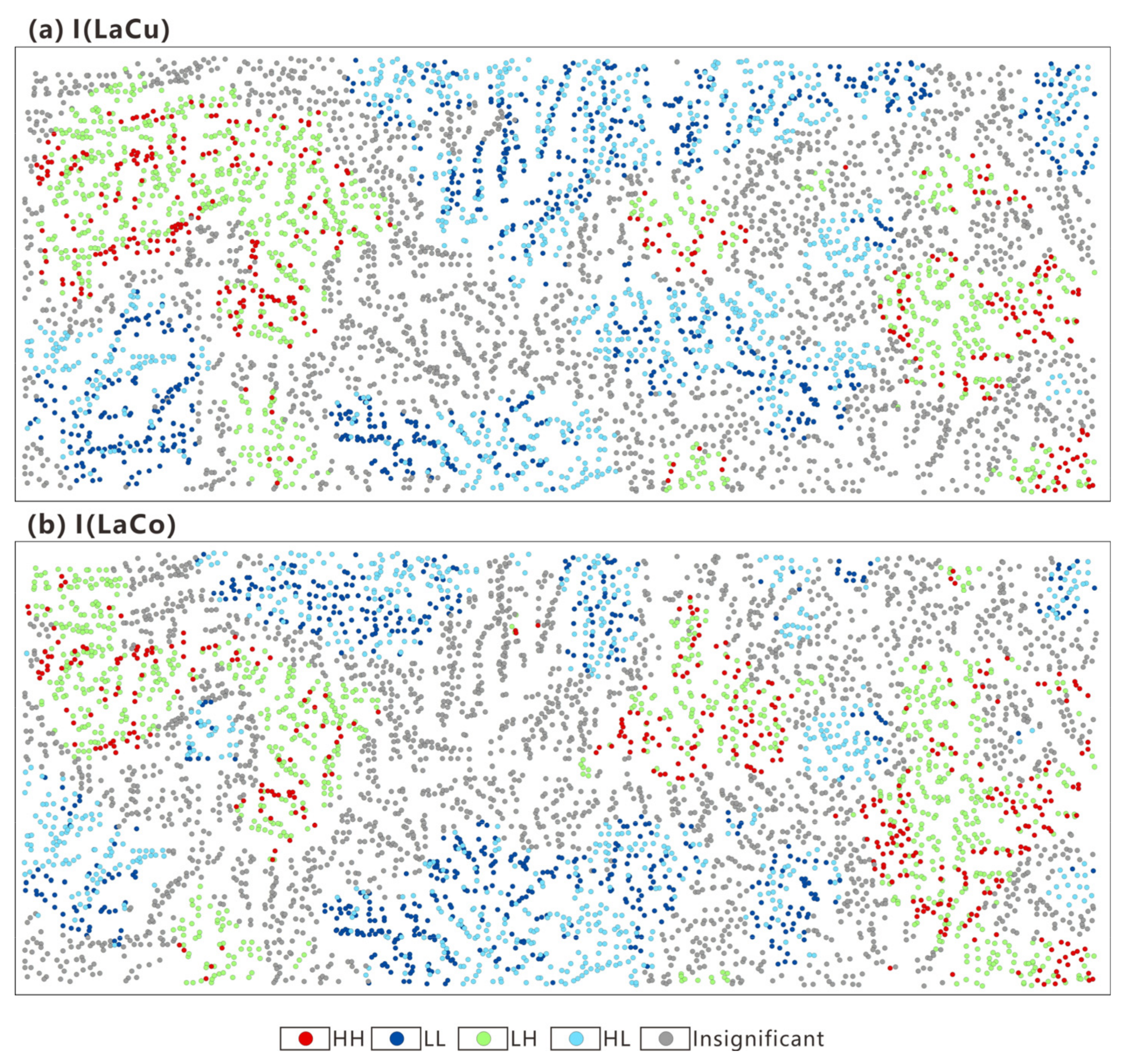
4.1.2. Bivariate Spatial Cross Correlation between Two Elements

The bivariate global Moran’s I for 15 elements in the study area are shown in Table 4, and all the calculated results passed the statistical significance test. We quantified the strength of spatial cross correlation between all element pairs, as shown in Table 4, the diagonal values of which are consistent with the univariate global Moran’s I. The elements with strong positive correlations include Pb and Cd, Pb and Zn, Cu and Bi, and Zn and Cd, and those with negative correlations include La and Co, and La and Cu (Table 5 and Table 6).
The clustering map of bivariate local Moran’s I divides the sampling points into five categories, i.e., insignificant, high–high (HH), low–low (LL), low–high (LH), and high–low (HL) clustered. However, their meanings are different from categories in a univariate clustering map. In the clustering map of bivariate local Moran’s I, I a b i indicates the spatial pattern of the related element, b , around the main element, a . From this, we plotted I CuCo , I CoCu , I CuBi , and I AsSb , as shown in Figure 10. In the I CuCo and I CoCu , the sampling points with high–high (HH) and low–low (LL) clustering are consistent with the univariate I Cu and I Co . Therefore, I CuCo and I CoCu show that the spatial distributions of Cu and Co in the study area are similar and positively cross-correlated. Due to the differences in the spatial distribution of Cu and Co, there are some differences in I CuCo and I CoCu after exchanging the main variable and related variable. The high–high (HH) clustering in I CuBi and I AsSb also has obvious regionality. Although these element pairs are globally positively cross-correlated, there are still some local negative cross-correlation (LH/HL) points beside mainly local positive cross-correlation points. The map for I LaCu and I LaCo is shown in Figure 11. There are apparent areas of low–high (LH) and high–low (HL) clustering in Figure 11, which indicate a negative cross correlation of the two elements. Although these two element pairs are globally negatively cross-correlated, there are still some local positive cross-correlation (HH/LL) points. Therefore, the bivariate local Moran’s I not only effectively reveals whether two elements have a spatial cross correlation but also helps us to better understand the spatial distribution pattern of coexistence of elements.

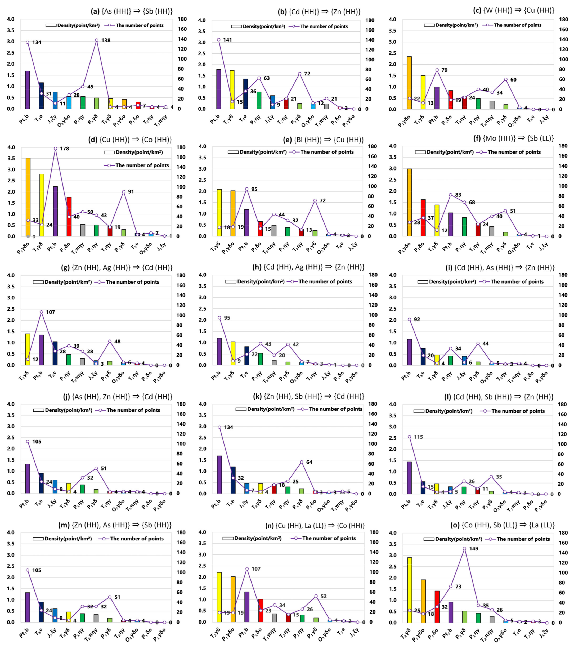
4.2. Association Rules among Multiple Elements

4.2.1. Association Rule Mining

The 4959 geochemical sampling points were each taken as an event in the Apriori algorithm. Then, we reorganized the geochemical concentration data into the original dataset, D, for association rule mining according to clustering by local univariate Moran’s I, as shown in Table 7. Table 8 shows the statistics for the LMIC analysis. Some items frequently appear in events, whereas some items are very sparse. If the support threshold in the Apriori algorithm is set too low, the efficiency of the mining algorithm is low, and a large number of meaningless rules may be extracted. If the support threshold is set too high, the efficiency of the mining algorithm is high, but it may filter out some sparse items. For this study, we set the support threshold a Smin = 0.05 and the confidence threshold at Cmin = 0.7.
We used the Apriori algorithm to mine out dozens of association rules, of which 15 rules were selected for interpretation (Table 9). The supports for Au and Pb in the Apriori algorithm are lower than the threshold, so no relevant association rules were mined. Meanwhile, the relevance of these association rules was judged according to the coexistence of elements and the geological environment in the study area.

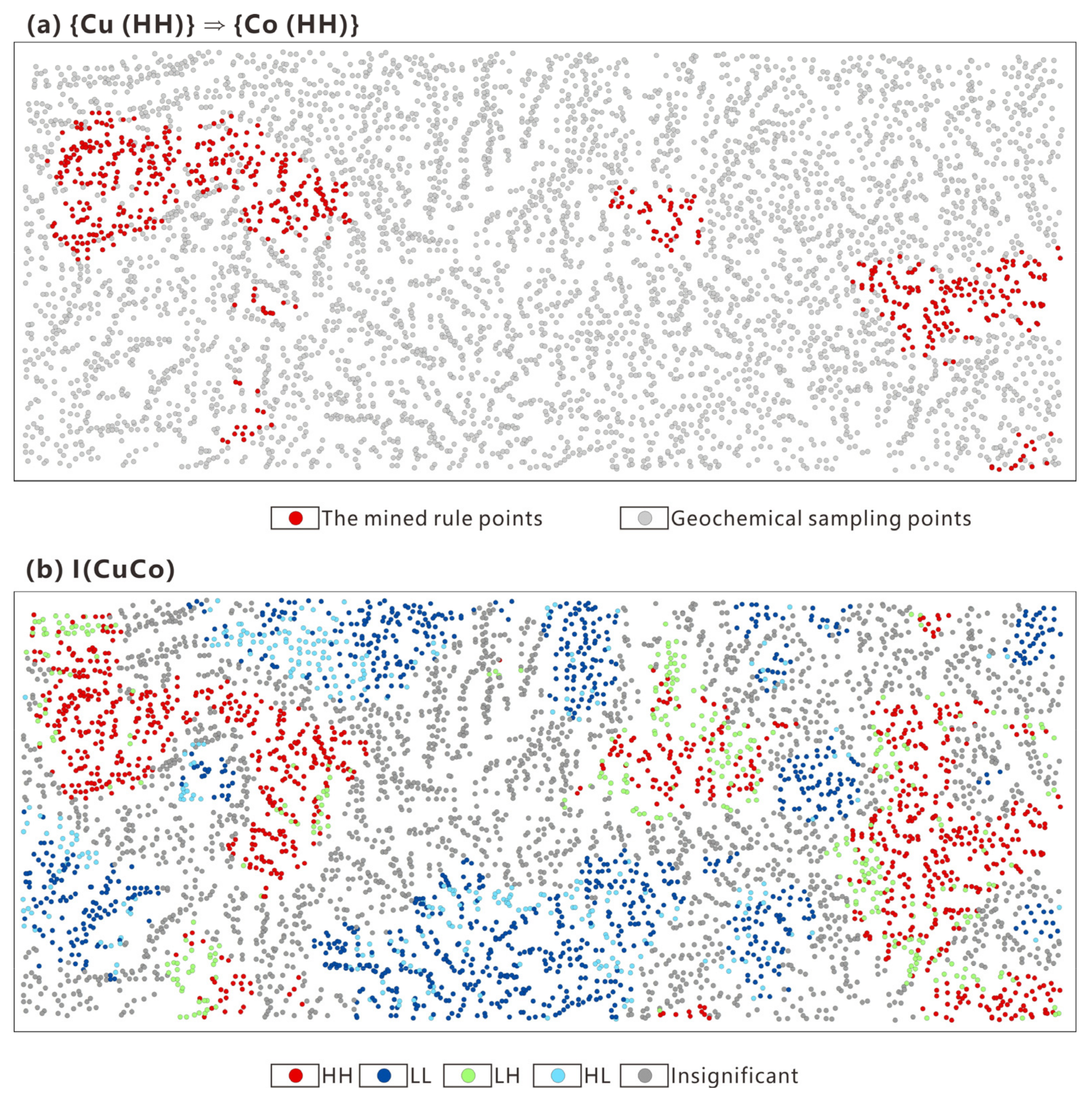
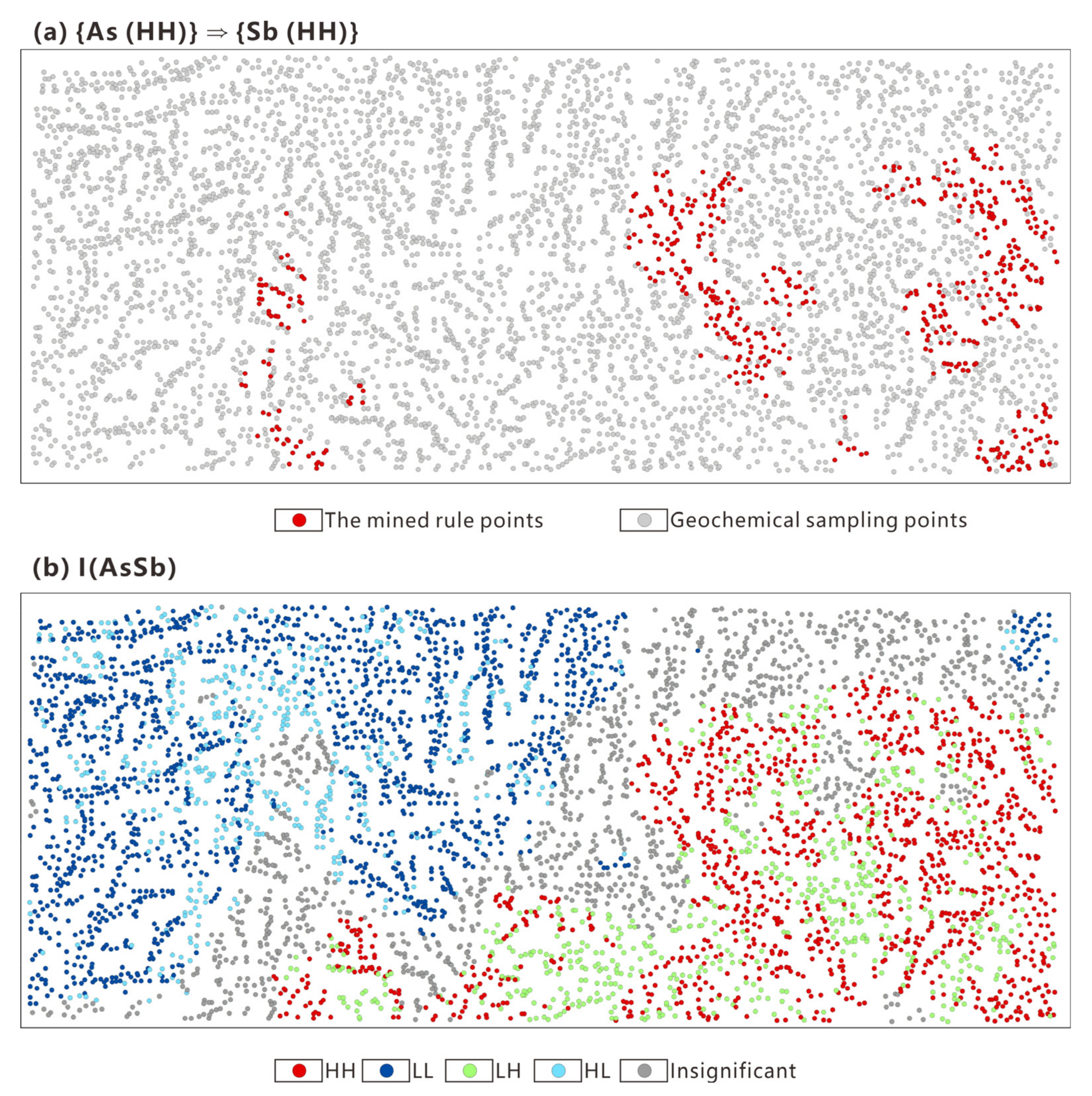
4.2.2. Comparison with Bivariate Spatial Cross Correlation

The affinity of elements is the ability of elements to preferentially coexist with each other. The most abundant anions in the crustal system are oxygen (O) and sulfur (S). Therefore, according to the geochemical affinities, the 15 elements are divided into the following three categories: (1) native elements, i.e., Au; (2) sulfides, i.e., Sn, Ag, As, Sb, Bi, Cu, Co, Pb, Zn, and Cd; and (3) oxides and lithophiles, i.e., Mo, Nb, W, and La.
The mining of association rules shows that there are positive correlations among all sulfophile elements with HH clustering, that is, {As (HH)} ⇒ {Sb (HH)}, {Cd (HH)} ⇒ {Zn (HH)}, {Cu (HH)} ⇒ {Co (HH)}, {Bi (HH)} ⇒ {Cu (HH)}, {Zn (HH), Ag (HH)} ⇒ {Cd (HH)}, {Cd (HH), Ag (HH)} ⇒ {Zn (HH)}, {Cd (HH), As (HH)} ⇒ {Zn (HH)}, {As (HH), Zn (HH)} ⇒ {Cd (HH)}, {Zn (HH), Sb (HH)} ⇒ {Cd (HH)}, {Cd (HH), Sb (HH)} ⇒ {Zn (HH)}, and {Zn (HH), As (HH)} ⇒ {Sb (HH)}. In rules {Mo (HH)} ⇒ {Sb (LL)}, {Cu (HH), La (LL)} ⇒ {Co (HH)}, and {Co (HH), Sb (LL)} ⇒ {La (LL)}, there are positive correlations between sulfophile elements with HH clustering and oxyphile elements with LL clustering.
We next compared the bivariate spatial cross correlations and association rules for Cu and Co (Figure 12), as well as As and Sb (Figure 13). The distributions of I CuCo HH clustering and I AsSb HH clustering are spatially similar to the association rules {Cu (HH)} ⇒ {Co (HH)} and {As (HH)} ⇒ {Sb (HH)}, respectively; however, I CuCo HH clustering and I AsSb HH clustering cover wider areas. In addition, I CuCo and I AsSb reveal not only high HH clustering but also LL, LH, and HL clustering, which shows the simultaneous relationship between two elements but does not scale efficiently to massive data sets. In contrast, association rule mining is suitable for revealing the association among items in a large geochemical dataset.

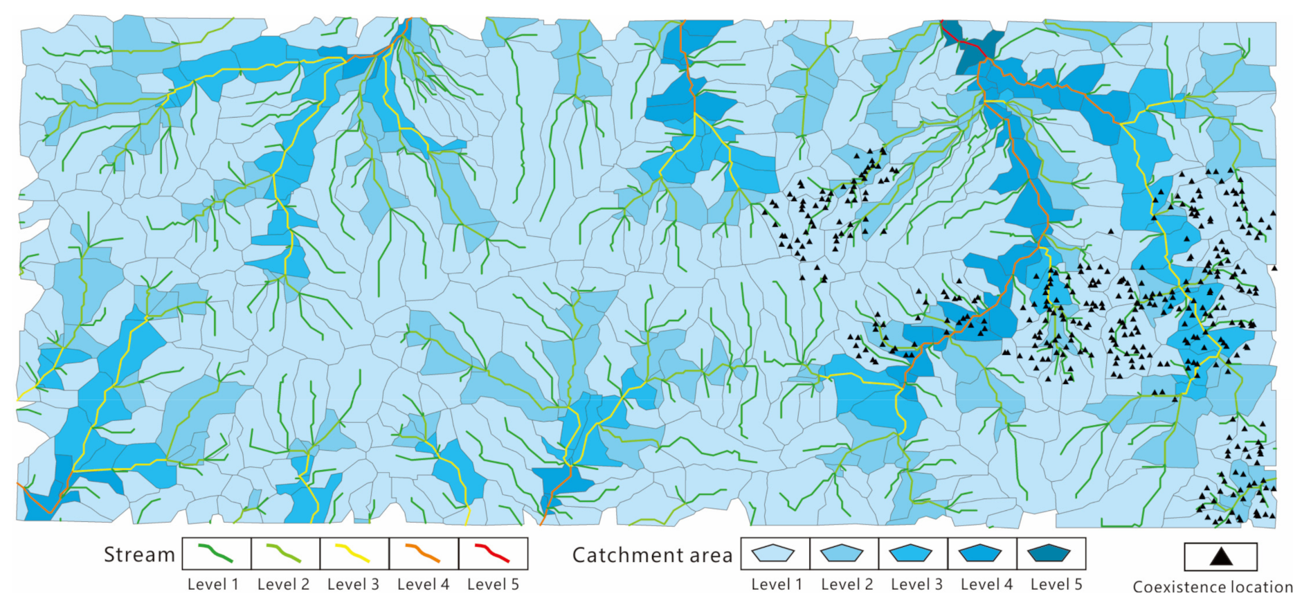
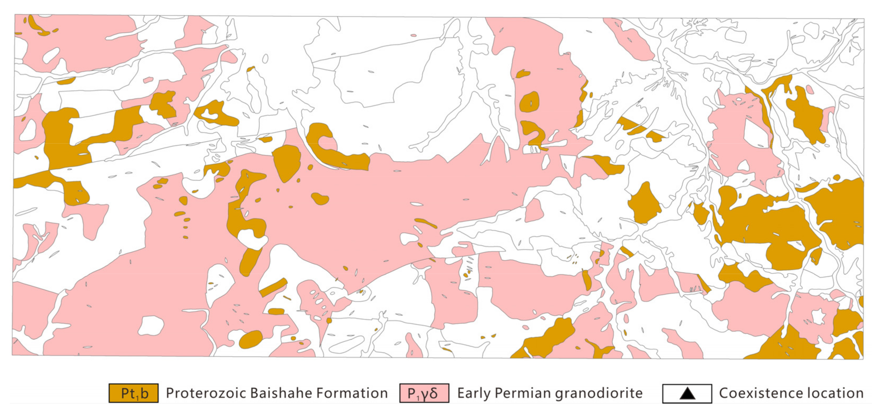
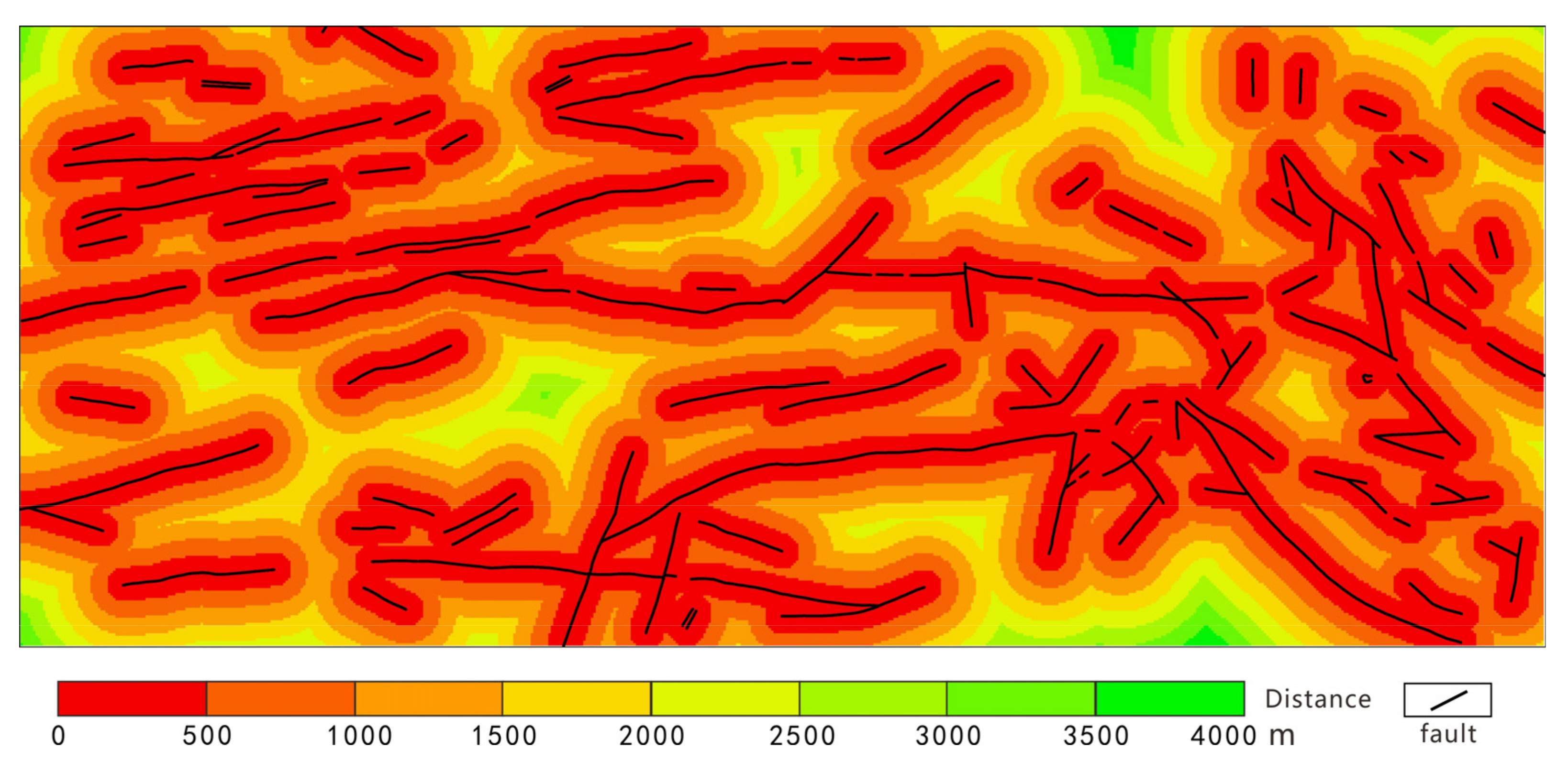
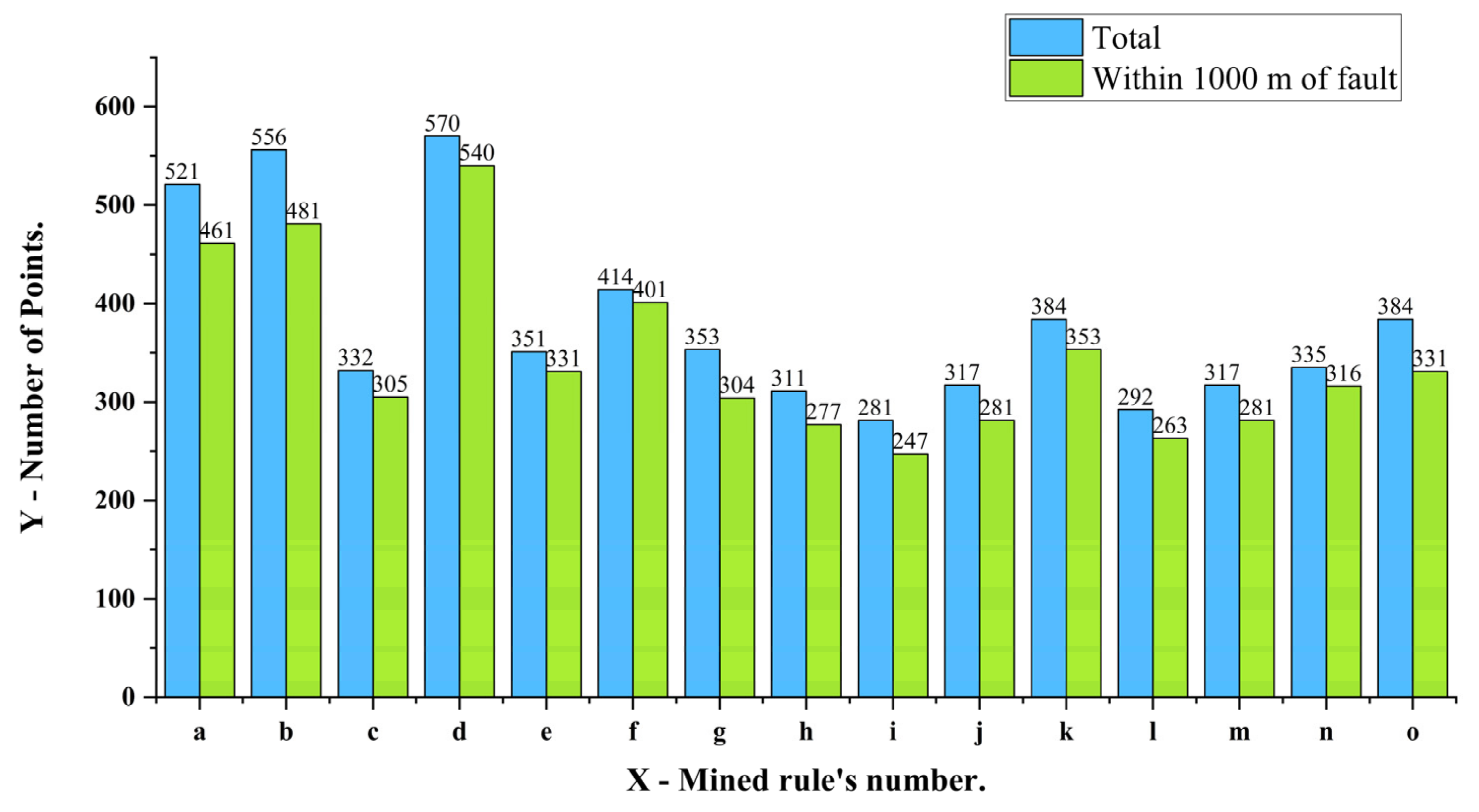
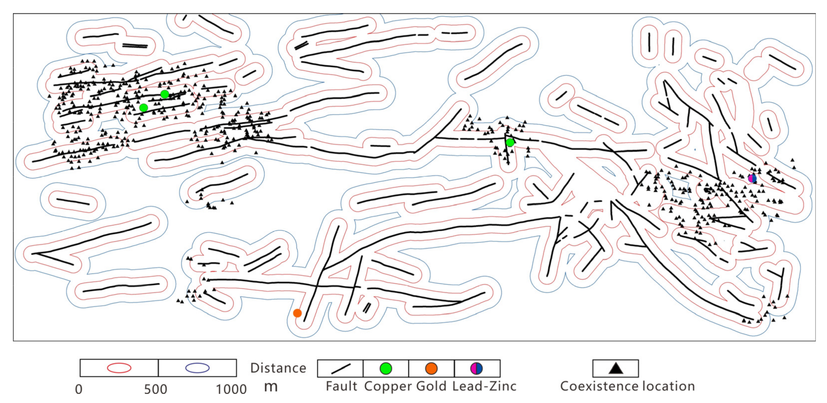
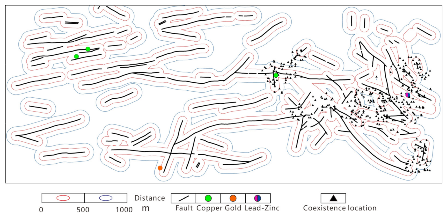
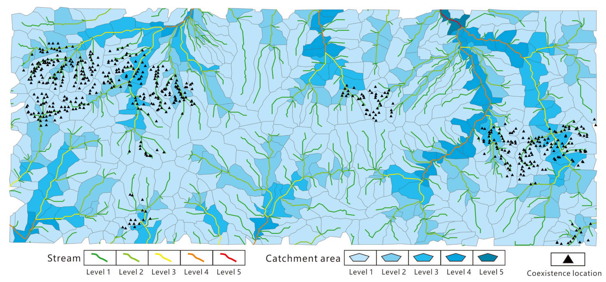
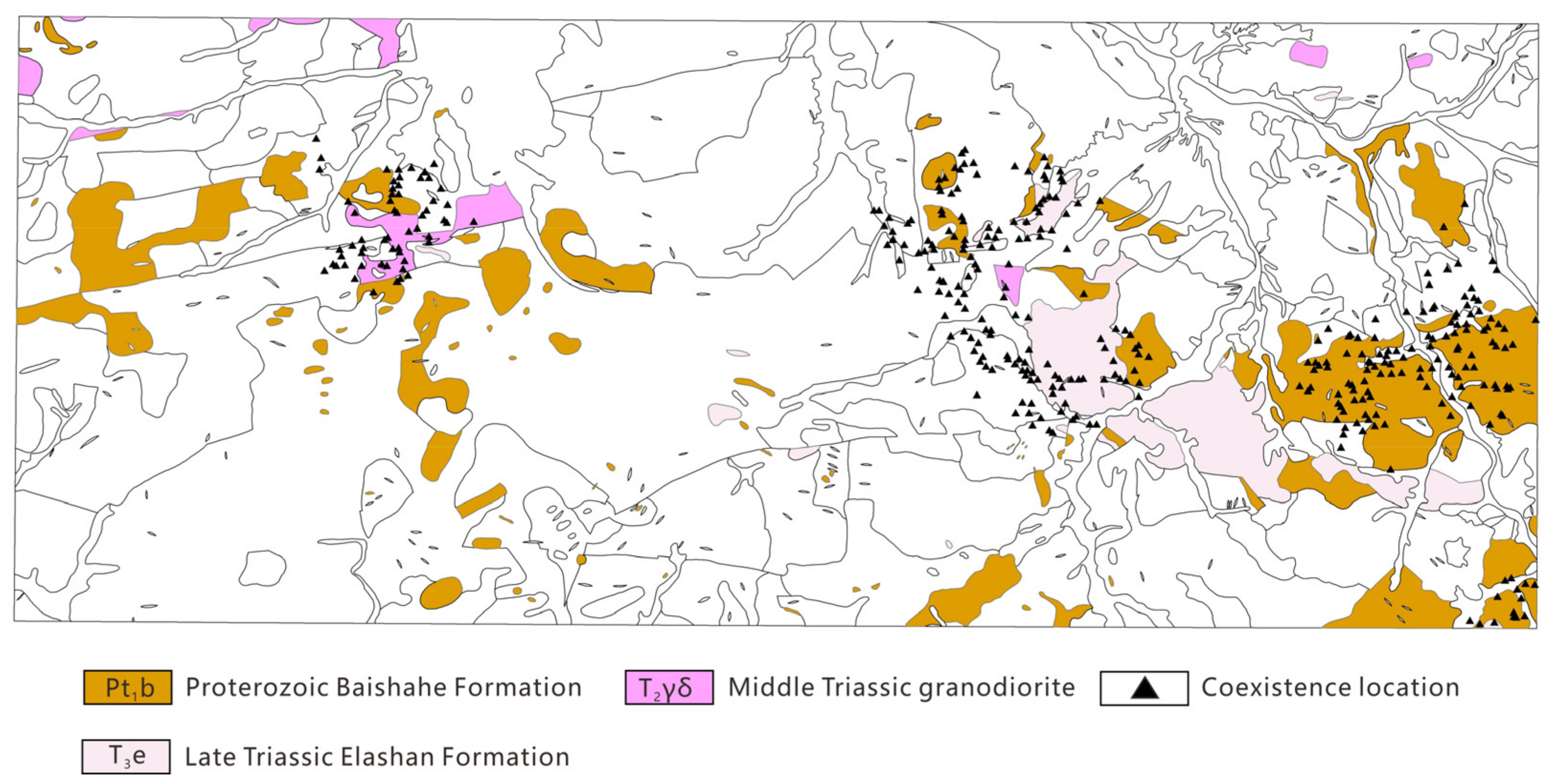
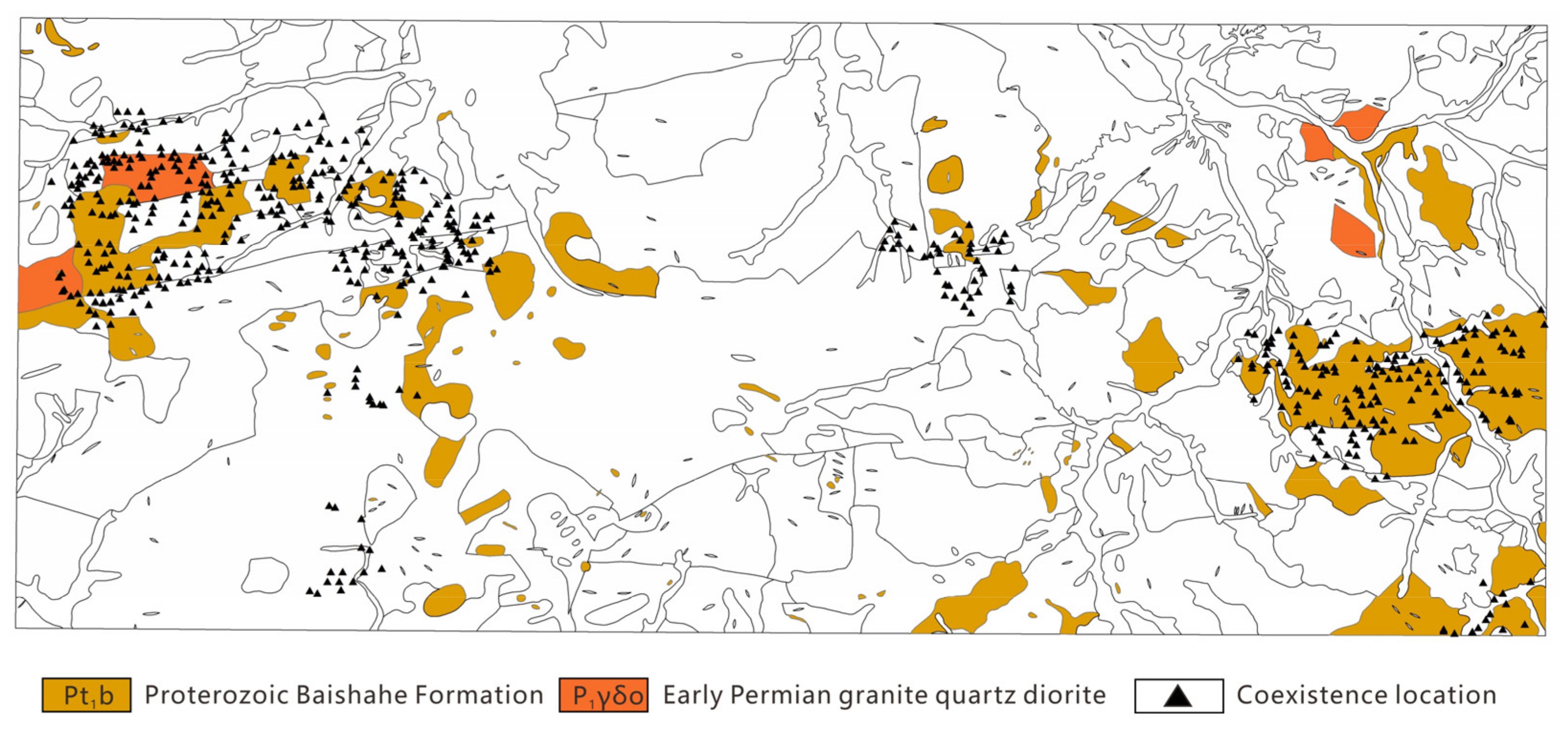
4.2.3. Controls of Geological Features

Due to the influence of multiple stages of tectonic and magmatic activities, the fault structures in the study area are relatively well developed. We calculated the Euclidean distance field for the faults in the study area (Figure 14). Then, the 15 mined association rules were overlaid with the fault distance field (Figure 15). We found that more than 86% of the mined rule points are located within 1000 m distance of the fault, especially {Cu (HH)} ⇒ {Co (HH)} (Figure 16) and {Zn (HH), Sb (HH)} ⇒ {Cd (HH)} (Figure 17). The rule {Cu (HH)} ⇒ {Co (HH)} is most predominant near the faults in the northwest and southeast parts of the study area, and three known copper ore occurrences are also near the faults. The rule {Zn (HH), Sb (HH)} ⇒ {Cd (HH)} is most strongly associated with the faults in the southeastern part of the study area, and a known lead-zinc ore occurrence is near the faults. That is, the fault structure has an obvious control effect on clustering of the elements. Figure 16 and Figure 17 show that three copper ore occurrences and one lead-zinc ore occurrence all appear in areas with high densities of their corresponding association rule points. In addition, we extracted streams and catchment areas to analyze whether element co-occurrence is related to stream transport. As shown in Figure 18 and Figure 19, most {Cu (HH)} ⇒ {Co (HH)} and {Zn (HH), Sb (HH)} ⇒ {Cd (HH)} events are distributed in the upper reaches of the streams and catchment areas, so the impact of stream transport on element association rule mining is weak in the study area.
The mineralogical composition of lithological strata impacts the coexistence of elements. We overlaid the mined association rules with the geological map and counted the points and density of each rule in the main lithostrata (Figure 20). A greater density and number of points of association rules of sulfides and the related elements occurs in the Proterozoic Baishahe Formation (Pt1b) and the Early Permian granodiorite (P1γδ), especially {As (HH)} ⇒ {Sb (HH)}. The Proterozoic Baishahe Formation (Pt1b) is the basement rock series in the study area, which is divided into carbonate rock, schist, and gneiss. Due to the influence of multiple orogenic events and frequent magmatic activity, the Proterozoic Baishahe Formation (Pt1b) and various intrusive rocks show good metallogenic conditions and prospects in the study area. The Late Triassic Elashan Formation (T3e) is divided into andesite, dacite, and rhyolite. During this geological period, tectonic movements, volcanic eruptions, and structural fractures were developed, which were good storage places for later metallogenic materials. However, because the Late Triassic Elashan Formation is not the main source of metallogenic materials, we found that it is not strongly related to association rules. Figure 21 shows that rule {As (HH)} ⇒ {Sb (HH)} occurs not only in Pt1b but also in the contact zones between intrusive rocks of different ages and Pt1b.
According to the geological survey data, the enrichment of Cu, Pb, Zn, Ag, Bi, and other elements in the Proterozoic Baishahe Formation (Pt1b) provides the main ore-forming materials in the study area. The locations of rules {As (HH)} ⇒ {Sb (HH)}, {Zn (HH), Ag (HH)} ⇒ {Cd (HH)}, and {Cu (HH)} ⇒ {Co (HH)} are related to Pt1b, as shown in Figure 21, Figure 22 and Figure 23. The association rules of sulfophile elements, e.g., {As (HH)} ⇒ {Sb (HH)}, {Cd (HH)} ⇒ {Zn (HH)}, {Zn (HH), Ag (HH)} ⇒ {Cd (HH)}, {Cd (HH), Ag (HH)} ⇒ {Zn (HH)}, {Cd (HH), As (HH)} ⇒ {Zn (HH)}, {Cd (HH), As (HH)} ⇒ {Zn (HH)}, {Zn (HH), Sb (HH)} ⇒ {Cd (HH)}, {Cd (HH), Sb (HH)} ⇒ {Zn (HH)}, and {Zn (HH), As (HH)} ⇒ {Sb (HH)}, are mainly distributed in the Proterozoic Baishahe Formation (Pt1b), the Late Triassic Elashan Formation (T3e), and the Middle Triassic granodiorite (T2γδ). The Middle Triassic magmatism resulted in the intrusion of the middle Triassic Kekesai Sequence granite and the Late Triassic Zamari Sequence granite, which provided conditions for enrichment of many sulfophile elements in the study area, especially represented by the rule {Zn (HH), Ag (HH)} ⇒ {Cd (HH)} (Figure 22). Therefore, the Middle Triassic magmatism provided a heat and material source to enrich elements and is an important geological unit for aggregating sulfophile elements. Cu mineralization often occurs in the contact between the Early Permian magmatic rocks and surrounding rocks, such as the Proterozoic Baishahe Formation (Pt1b), forming the Keregou East copper occurrence and the Hariza copper deposit. The rules of {W (HH)} ⇒ {Cu (HH)}, {Cu (HH)} ⇒ {Co (HH)}, {Bi (HH)} ⇒ {Cu (HH)}, {Cu (HH), La (LL)} ⇒ {Co (HH)}, and {Co (HH), Sb (LL)} ⇒ {La (LL)} related to Cu HH and Co HH clustering also have high density in the Early Permian granite quartz diorite (P1γδο), especially {Cu (HH)} ⇒ {Co (HH)} (Figure 23). Therefore, we may infer that a coexisting relationship between Cu and other elements developed in the Early Permian granite quartz diorite.

5. Conclusions

Our case study of association rule mining in the Chahanwusu River area yielded the following conclusions.
(1) According to the global autocorrelation indicators, Au shows a random distribution in the study area, and 14 other elements have positive correlations, ranked from large to small: Sb, Zn, Pb, Cu, Cd, As, Sn, Bi, Ag, Mo, Co, W, La, and Nb. Compared with local Geary’s C and local Getis–Ord’s G, local Moran’s I can identify points of HH, LL, LH, and HL clustering with a precise meaning for each category, which makes it a better local autocorrelation indicator for association rule mining.
(2) Based on the univariate LMIC results, the proposed method successfully mined 15 association rules among various elements in the study area. Bivariate spatial cross correlation can also detect distribution-pattern details of the co-occurrence of pair elements compared with association rule mining. However, it cannot be used to efficiently explore massive geochemical datasets. In contrast, association rule mining can reveal the association among items in a large geochemical dataset.
(3) Overlying the mining results of association rules on the faults, ore occurrences, and catchment areas, we found that more than 86% of the mined rule points are located within 1000 m of faults and near known ore occurrences, and the impact of stream transport on element co-occurrences is weak. Greater densities and numbers of points of association rules were found in the Proterozoic Baishahe Formation (Pt1b) and the Early Permian granodiorite (P1γδ). Therefore, the association rules are closely related to specific geological features.
The association rules mined in this paper are mainly high-value element co-occurrence. Where these combinations appear, higher concentrations of the element are more likely, which can improve the prediction of unknown ore deposits or occurrences. However, the mining efficiency of low-value element co-occurrence is low, and the local dilution of elements in the study area cannot be effectively detected. In the future, we will build an element-association rule database to find combinations of anomalies for known metallogenic elements and to map the probability of unknown mineralization in the study area.

Author Contributions

Conceptualization, B.Z. and J.D.; methodology, Y.C.; software, Z.J. and N.C.; validation, B.Z., Z.J. and Y.C.; data curation, Y.C.; writing—original draft preparation, B.Z. and Z.J.; writing—review and editing, B.Z. and U.K.; funding acquisition, B.Z. All authors have read and agreed to the published version of the manuscript.

Funding

This study was supported by grants from the National Natural Science Foundation of China (Grant Nos. 42072326 and 41772348), China Geological Survey Project (Grant No. DD20190156), and the National Key Research and Development Program of China (Grant No. 2019YFC1805905).

Institutional Review Board Statement

Not applicable.

Informed Consent Statement

Not applicable.

Data Availability Statement

The dataset of the current study is not publicly available due to a data privacy agreement we signed with The 8th Team of Qinghai Provincial Bureau of Nonferrous Metals and Geological Exploration but are available from the corresponding author on reasonable request.

Acknowledgments

The authors would like to thank the Co-Construction MapGIS Library by Engineering Research Center for Geographic Information System of China and Central South University for providing MapGIS® software (Wuhan Zondy Cyber-Tech Co., Ltd., Wuhan, China). We also thank ZHANG Shao-ning (The 8th Team of Qinghai Provincial Bureau of Nonferrous Metals and Geological Exploration) and LAI Jian-qing (Central South University) for their kind assistance with data collection and Jeffrey Dick (Central South University) for revising scientific English writing of this manuscript.

Conflicts of Interest

The authors declare no conflict of interest.

References

  1. Korobova, E.M.; Romanov, S.L. A Chernobyl 137Cs contamination study as an example for the spatial structure of geochemical fields and modeling of the geochemical field structure. Chemom. Intell. Lab. Syst. 2009, 99, 1–8. [Google Scholar] [CrossRef]
  2. Zhang, B.; Chen, Y.; Huang, A.; Lu, H.; Cheng, Q. Geochemical field and its roles on the 3D prediction of concealed ore-bodies. Acta Petrol. Sin. 2018, 34, 352–362. [Google Scholar]
  3. Tobler, W.R. A computer movie simulating urban growth in the Detroit region. Econ. Geogr. 1970, 46, 234–240. [Google Scholar] [CrossRef]
  4. Moran, P.A. Notes on continuous stochastic phenomena. Biometrika 1950, 37, 17–23. [Google Scholar] [CrossRef]
  5. Geary, R.C. The Contiguity Ratio and Statistical Mapping. Inc. Stat. 1954, 5, 115–146. [Google Scholar] [CrossRef]
  6. Cliff, A.D.; Ord, J.K. The Problem of Spatial Autocorrelation. Reg. Sci. 1969, 1, 26–55. [Google Scholar]
  7. Cliff, A.D.; Ord, J.K. Evaluating the percentage points of a spatial autocorrelation coefficient. Geogr. Anal. 1971, 3, 51–62. [Google Scholar] [CrossRef]
  8. Cliff, A.D.; Ord, J.K. Spatial Processes: Models & Applications; Taylor & Francis: Oxford, UK, 1981. [Google Scholar]
  9. Getis, A.; Ord, J.K. The Analysis of Spatial Association by Use of Distance Statistics; Springer: Berlin/Heidelberg, Germany, 2010; pp. 127–145. [Google Scholar]
  10. Ord, J.K.; Getis, A. Local spatial autocorrelation statistics: Distributional issues and an application. Geogr. Anal. 1995, 27, 286–306. [Google Scholar] [CrossRef]
  11. Anselin, L. Local indicators of spatial association—LISA. Geogr. Anal. 1995, 27, 93–115. [Google Scholar] [CrossRef]
  12. Boots, B.; Okabe, A. Local statistical spatial analysis: Inventory and prospect. Int. J. Geogr. Inf. Sci. 2007, 21, 355–375. [Google Scholar] [CrossRef]
  13. Anselin, L. A local indicator of multivariate spatial association: Extending Geary’s C. Geogr. Anal. 2019, 51, 133–150. [Google Scholar] [CrossRef]
  14. Goovaerts, P.; Jacquez, G.M. Accounting for regional background and population size in the detection of spatial clusters and outliers using geostatistical filtering and spatial neutral models: The case of lung cancer in Long Island, New York. Int. J. Health Geogr. 2004, 3, 14. [Google Scholar] [CrossRef] [PubMed] [Green Version]
  15. McLaughlin, C.C.; Boscoe, F.P. Effects of randomization methods on statistical inference in disease cluster detection. Health Place 2007, 13, 152–163. [Google Scholar] [CrossRef] [PubMed]
  16. Yu, X.; Wang, S.; Wang, H.; Liang, Y.; Chen, S.; Wu, K.; Yang, Z.; Li, C.; Chang, Y.; Zhan, Y. Detection of Geochemical Element Assemblage Anomalies Using a Local Correlation Approach. J. Earth Sci. 2021, 32, 408–414. [Google Scholar] [CrossRef]
  17. Xiao, G.; Hu, Y.; Li, N.; Yang, D. Spatial autocorrelation analysis of monitoring data of heavy metals in rice in China. Food Control 2018, 89, 32–37. [Google Scholar] [CrossRef]
  18. Bivand, R.S.; Wong, D.W. Comparing implementations of global and local indicators of spatial association. Test 2018, 27, 716–748. [Google Scholar] [CrossRef]
  19. Cheng, Q. Singularity theory and methods for mapping geochemical anomalies caused by buried sources and for predicting undiscovered mineral deposits in covered areas. J. Geochem. Explor. 2012, 122, 55–70. [Google Scholar] [CrossRef]
  20. Carranza, E.J.M. Geochemical Anomaly and Mineral Prospectivity Mapping in GIS; Elsevier: Amsterdam, The Netherlands, 2008. [Google Scholar]
  21. Zuo, R.; Xiong, Y. Geodata science and geochemical mapping. J. Geochem. Explor. 2019, 209, 106431. [Google Scholar] [CrossRef]
  22. Wang, J.; Zhou, Y.; Xiao, F. Identification of multi-element geochemical anomalies using unsupervised machine learning algorithms: A case study from Ag–Pb–Zn deposits in north-western Zhejiang, China. Appl. Geochem. 2020, 120, 104679. [Google Scholar] [CrossRef]
  23. Taylor, R.; Steven, T. Definition of mineral resource potential. Econ. Geol. 1983, 78, 1268–1270. [Google Scholar] [CrossRef]
  24. Wang, L.; Wu, X.; Zhang, B.; Li, X.; Huang, A.; Meng, F.; Dai, P. Recognition of Significant Surface Soil Geochemical Anomalies Via Weighted 3D Shortest-Distance Field of Subsurface Orebodies: A Case Study in the Hongtoushan Copper Mine, NE China. Nat. Resour. Res. 2019, 28, 587–607. [Google Scholar] [CrossRef]
  25. Hawkes, H.E.; Webb, J.S. Geochemistry in mineral exploration. Soil Sci. 1963, 95, 283. [Google Scholar] [CrossRef]
  26. Sinclair, A. Selection of threshold values in geochemical data using probability graphs. J. Geochem. Explor. 1974, 3, 129–149. [Google Scholar] [CrossRef]
  27. Govett, G.; Goodfellow, W.; Chapman, R.; Chork, C. Exploration geochemistry—distribution of elements and recognition of anomalies. J. Int. Assoc. Math. Geol. 1975, 7, 415–446. [Google Scholar] [CrossRef]
  28. El-Makky, A.M. Statistical analyses of La, Ce, Nd, Y, Nb, Ti, P, and Zr in bedrocks and their significance in geochemical exploration at the Um Garayat Gold mine area, Eastern Desert, Egypt. Nat. Resour. Res. 2011, 20, 157. [Google Scholar] [CrossRef]
  29. Ravani, P.; Barrett, B.J.; Parfrey, P.S. Longitudinal Studies 2: Modeling Data Using Multivariate Analysis. Methods Mol. Biol. Clifton NJ 2021, 2249, 103–124. [Google Scholar]
  30. Cox, D.R.; Snell, E.J. Analysis of Binary Data; Routledge: London, UK, 2018. [Google Scholar]
  31. Cioci, A.C.; Cioci, A.L.; Mantero, A.M.; Parreco, J.P.; Yeh, D.D.; Rattan, R. Advanced statistics: Multiple logistic regression, Cox proportional hazards, and propensity scores. Surg. Infect. 2021, 22, 604–610. [Google Scholar] [CrossRef]
  32. Agterberg, F.P. Computer programs for mineral exploration. Science 1989, 245, 76–81. [Google Scholar] [CrossRef]
  33. Cheng, Q.; Agterberg, F. Fuzzy weights of evidence method and its application in mineral potential mapping. Nat. Resour. Res. 1999, 8, 27–35. [Google Scholar] [CrossRef]
  34. Goyes-Penafiel, P.; Hernandez-Rojas, A. Double landslide susceptibility assessment based on artificial neural networks and weights of evidence. Bol. Geol. 2021, 43, 173–191. [Google Scholar]
  35. Cheng, Q.; Agterberg, F.; Ballantyne, S. The separation of geochemical anomalies from background by fractal methods. J. Geochem. Explor. 1994, 51, 109–130. [Google Scholar] [CrossRef]
  36. Cheng, Q.; Xu, Y.; Grunsky, E. Integrated spatial and spectrum method for geochemical anomaly separation. Nat. Resour. Res. 2000, 9, 43–52. [Google Scholar] [CrossRef]
  37. Cheng, Q. Mapping singularities with stream sediment geochemical data for prediction of undiscovered mineral deposits in Gejiu, Yunnan Province, China. Ore Geol. Rev. 2007, 32, 314–324. [Google Scholar] [CrossRef]
  38. Goovaerts, P. Geostatistical modelling of spatial uncertainty using p-field simulation with conditional probability fields. Int. J. Geogr. Inf. Sci. 2002, 16, 167–178. [Google Scholar] [CrossRef]
  39. Naik, M.R.; Barik, M.; Prasad, K.; Kumar, A.; Verma, A.K.; Sahoo, S.K.; Jha, V.; Sahoo, N.K. Hydro-geochemical analysis based on entropy and geostatistics model for delineation of anthropogenic ground water pollution for health risks assessment of Dhenkanal district, India. Ecotoxicology 2021, 2, 43–52. [Google Scholar] [CrossRef] [PubMed]
  40. Zuo, R.; Carranza, E.J.M. Support vector machine: A tool for mapping mineral prospectivity. Comput. Geosci. 2011, 37, 1967–1975. [Google Scholar] [CrossRef]
  41. Xiong, J.; Li, J.; Cheng, W.; Wang, N.; Guo, L. A GIS-based support vector machine model for flash flood vulnerability assessment and mapping in China. ISPRS Int. J. Geo-Inf. 2019, 8, 297. [Google Scholar] [CrossRef] [Green Version]
  42. Rodriguez-Galiano, V.; Chica-Olmo, M.; Chica-Rivas, M. Predictive modelling of gold potential with the integration of multisource information based on random forest: A case study on the Rodalquilar area, Southern Spain. Int. J. Geogr. Inf. Sci. 2014, 28, 1336–1354. [Google Scholar] [CrossRef]
  43. Zhang, B.; Li, M.; Li, W.; Jiang, Z.; Khan, U.; Wang, L.; Wang, F. Machine learning strategies for lithostratigraphic classification based on geochemical sampling data: A case study in the area of the Chahanwusu River, Qinghai Province, China. J. Cent. South Univ. 2021, 28, 1422–1447. [Google Scholar] [CrossRef]
  44. Porwal, A.; Carranza, E.J.M. Classifiers for Modeling of Mineral Potential; Wiley-Blackwell: Hoboken, NJ, USA, 2008. [Google Scholar]
  45. Porwal, A.; Carranza, E.J.M.; Hale, M. Bayesian network classifiers for mineral potential mapping. Comput. Geosci. 2006, 32, 1–16. [Google Scholar] [CrossRef]
  46. Klüppelberg, C.; Krali, M. Estimating an extreme Bayesian network via scalings. J. Multivar. Anal. 2021, 181, 104672. [Google Scholar] [CrossRef]
  47. Xiong, Y.; Zuo, R. Recognition of geochemical anomalies using a deep autoencoder network. Comput. Geosci. 2016, 86, 75–82. [Google Scholar] [CrossRef]
  48. Nguyen, T.T.; Liu, X.; Ren, Z. A study of geochemical exploration spational cluster identification based on local spatial autocorrelation. Geophys. Geochem. Explor. 2014, 38, 370–376. [Google Scholar]
  49. Wang, H.; Cheng, Q.; Zuo, R. Spatial characteristics of geochemical patterns related to Fe mineralization in the southwestern Fujian province (China). J. Geochem. Explor. 2015, 148, 259–269. [Google Scholar] [CrossRef]
  50. Ji, B.; Zhou, T.; Yuan, F.; Zhang, D.; Liu, L.; Liu, G. A method for identifying geochemical anomalies based on spatial autocorrelation. Sci. Surv. Mapp. 2017, 42, 24–27. [Google Scholar]
  51. Sadeghi, M.; Morris, G.A.; Carranza, E.J.M.; Ladenberger, A.; Andersson, M. Rare earth element distribution and mineralization in Sweden: An application of principal component analysis to FOREGS soil geochemistry. J. Geochem. Explor. 2013, 133, 160–175. [Google Scholar] [CrossRef]
  52. Wang, J.; Zuo, R. Quantifying the Distribution Characteristics of Geochemical Elements and Identifying Their Associations in Southwestern Fujian Province, China. Minerals 2020, 10, 183. [Google Scholar] [CrossRef] [Green Version]
  53. Zhang, C.-S.; Li, Y. Extension of local association rules mining algorithm based on apriori algorithm. In Proceedings of the 2014 5th IEEE International Conference on Software Engineering and Service Science (ICSESS), Beijing, China, 27–29 June 2014; pp. 340–343. [Google Scholar]
  54. Zhang, X. Study of an improved Apriori algorithm for data mining of association rules. In Proceedings of the International Conference on Applied Science & Engineering Innovation, Jinan, China, 30–31 August 2015. [Google Scholar]
  55. Xu, T.; Dong, X. Mining frequent patterns with multiple minimum supports using basic Apriori. In Proceedings of the 2013 Ninth International Conference on Natural Computation (ICNC), Shenyang, China, 23–25 July 2013; pp. 957–961. [Google Scholar]
  56. Wu, X.; Kumar, V.; Quinlan, J.R.; Ghosh, J.; Yang, Q.; Motoda, H.; McLachlan, G.J.; Ng, A.; Liu, B.; Philip, S.Y. Top 10 algorithms in data mining. Knowl. Inf. Syst. 2008, 14, 1–37. [Google Scholar] [CrossRef] [Green Version]
  57. Agrawal, R.; Imieliński, T.; Swami, A. Mining association rules between sets of items in large databases. In Proceedings of the 1993 ACM SIGMOD International Conference on Management of Data, Washington, DC, USA, 25–28 May 1993; pp. 207–216. [Google Scholar]
  58. Liu, X.; Zhou, Y. Application of association rule algorithm in studying abnormal elemental associations in the Pangxidong area in western Guangdong Province, China. Earth Sci. Front. 2019, 26, 57–71. [Google Scholar]
  59. Qinghai Geological Survey Institute. Comprehensive Survey Report of 1:50000 Regional Mineral Geology, Stream Sediment Geochemistry and High-Precision Magnetic Survey in the Chahanwusu River Area, Dulan County, Qinghai Province; Qinghai Geological Survey Institute: Xining, China, 2008; pp. 254–273. [Google Scholar]
  60. Chou, Y.H. Spatial pattern and spatial autocorrelation. In Proceedings of the International Conference on Spatial Information Theory, Semmering, Austria, 21–23 September 1995; pp. 365–376. [Google Scholar]
  61. Buja, A.; Cook, D.; Swayne, D.F. Interactive high-dimensional data visualization. J. Comput. Graph. Stat. 1996, 5, 78–99. [Google Scholar]
  62. Anselin, L.; Syabri, I.; Smirnov, O. Visualizing multivariate spatial correlation with dynamically linked windows. In Proceedings of the Proceedings, CSISS Workshop on New Tools for Spatial Data Analysis, Santa Barbara, CA, USA, 22–26 July 2002. [Google Scholar]
Figure 1. Geological map of the study area, modified from [43].
Applsci 12 02247 g001
Figure 2. Map of stream sediment geochemical sampling points.
Applsci 12 02247 g002
Figure 3. Log-frequency distribution histogram of the 15 elements in the study area: (a) Au, (b) Sn, (c) Ag, (d) As, (e) Sb, (f) Bi, (g) Co, (h) Cu, (i) La, (j) Pb, (k) Zn, (l) W, (m) Mo, (n) Nb, and (o) Cd.
Applsci 12 02247 g003
Figure 4. Average concentrations of main mineralization elements in bedrock, e.g., (a) the Baishahe Formation, (b) the Elashan Formation, (c) monzogranite, (d) alkali feldspar granite, (e) monzogranite porphyry, (f) granodiorite, (g) quartz granodiorite, and (h) quartz diorite and their corresponding overlaying stream sediments, modified from [43].
Applsci 12 02247 g004
Figure 5. Algorithm for generating frequent itemsets.
Applsci 12 02247 g005
Figure 6. Algorithm for extracting strong association rules based on frequent itemsets.
Applsci 12 02247 g006
Figure 7. Voronoi diagrams of local Moran’s I indicators for major elements.
Applsci 12 02247 g007
Figure 8. LISA significance map of local Moran’s I indicators for major elements.
Applsci 12 02247 g008
Figure 9. Clustering map of local Moran’s I indicators for major elements.
Applsci 12 02247 g009
Figure 10. Clustering map of bivariate local Moran’s I with mainly positive cross correlation.
Applsci 12 02247 g010
Figure 11. Clustering map of bivariate local Moran’s I with mainly negative cross correlation.
Applsci 12 02247 g011
Figure 12. (a) Association rule mining result, {Cu (HH)} ⇒ {Co (HH)}, and (b) bivariate spatial cross-correlation indicator, I CuCo , of Cu and Co.
Applsci 12 02247 g012
Figure 13. (a) Association rule mining result, {As (HH)} ⇒ {Sb (HH)}, and (b) bivariate spatial cross-correlation indicator, I AsSb , of As and Sb.
Applsci 12 02247 g013
Figure 14. Euclidean distance field of faults.
Applsci 12 02247 g014
Figure 15. Number of mined rule points that are close to faults.
Applsci 12 02247 g015
Figure 16. Rule {Cu (HH)} ⇒ {Co (HH)} points within 500 m and 1000 m of faults.
Applsci 12 02247 g016
Figure 17. Rule {Zn (HH), Sb (HH)} ⇒ {Cd (HH)} points within 500 m and 1000 m of faults.
Applsci 12 02247 g017
Figure 18. Rule {Cu (HH)} ⇒ {Co (HH)} points overlayed with streams and catchment areas.
Applsci 12 02247 g018
Figure 19. Rule {Zn (HH), Sb (HH)} ⇒ {Cd (HH)} points overlayed with streams and catchment areas.
Applsci 12 02247 g019
Figure 20. Total number of points and density of each mined rule in the main lithostrata.
Applsci 12 02247 g020
Figure 21. Rule {As (HH)} ⇒ {Sb (HH)} overlayed with the main lithostrata.
Applsci 12 02247 g021
Figure 22. Rule {Zn (HH), Ag (HH)} ⇒ {Cd (HH)} overlayed with the main lithostrata.
Applsci 12 02247 g022
Figure 23. Rule {Cu (HH)} ⇒ {Co (HH)} overlayed with the main lithostrata.
Applsci 12 02247 g023
Table 1. Main statistical results of the stream-sediment elements in the study area.
ElementMeanMedianStandard DeviationSkewnessKurtosisCoefficient of Variation
Au1.421.201.8125.07793.151.27
Sn2.311.703.2110.35134.681.39
Ag76.3141.00117.356.7767.021.54
As13.078.1021.8913.21303.481.68
Sb0.820.471.4514.56372.591.88
Bi0.370.171.0013.68256.652.50
Co7.076.403.443.0724.090.48
Cu16.0512.1020.4415.15330.621.27
La13.7312.008.308.99192.650.61
Pb17.0012.8021.2913.35314.691.25
Zn48.2940.4032.064.2727.610.66
W2.741.705.9918.99528.952.22
Mo1.200.961.369.31117.221.17
Nb3.933.302.264.5337.900.59
Cd0.150.100.185.2849.300.85
Au, Ag: 10−9, others: 10−6.
Table 2. Spatial autocorrelation statistics.
Spatial Autocorrelation StatisticsCalculation FormulaRemarksReferences
global Moran’s I I = n i n j n w i j x i x ¯ x j x ¯ i n j n w i j i n x i x ¯ 2 The range of I is [−1, 1], I < 0 indicates negative spacial autocorrelation, I > 0 indicates positive spacial autocorrelation, and I tends to 0 indicates spatial random distribution.[4,6,7,8]
global Geary’s C C = n 1 i n j n w i j x i x j 2 2 i n j m w i j i n x i x ¯ 2   The range of C is [0, 2] C > 1 indicates indicates negative spatial autocorrelation, C < 1 indicates positive spatial autocorrelation, and C tends to 1 indicates spatial random distribution.[5,6,8]
global Getis–Ord’s G G = i n j n w i j x i x j i n j n x i x j     G < mathematical expectation (ME) indicates low value clustered, G > ME indicates high value clustered, and G tends to ME indicates spatial random distribution.[9]
local Moran’s I I i = x i x ¯ S 2 j n w i j x j x ¯
S 2 = i n x i x ¯ 2 n  
Z I i < 0 indicates negative spatial autocorrelation, Z I i > 0 indicates positive spatial auto-correlation, and Z I i tends to 0 indicates spatial random distribution.[9]
local Geary’s C C i = 1 S 2 j n w i j x i x j 2
S 2 = i n x i x ¯ 2 n
Z C i < 0 indicates negative spatial autocorrelation, and Z C i > 0 indicates positive spatial autocorrelation, and Z C i tends to 0 indicates spatial random distribution.[11]
local Getis–Ord’s G G i = j n w i j x j / j n x j   Z G i < 0 indicates negative spatial autocorrelation, Z G i > 0 indicates positive spatial autocorrelation, and Z G i tends to 0 indicates spatial random distribution.[9]
  x i and x j are the observed value at positions i and j , respectively; x j is x i position’s neighbor point at a certain distance; n is the total number of observations; x ¯ is the mean value of the observations; w i j is the spatial weight matrix; Z Γ = Γ E Γ / V A R Γ , Γ is a spatial statistic; E Γ is the mathematical expectation of Γ ; and V A R Γ is the variance of Γ .
Table 3. Univariate global spatial autocorrelation indicators for 15 elements in the study area.
VariableGlobal Moran’s IGlobal Geary’s CGlobal Getis–Ord’s G
Ip-Value (×10−16)Cp-Value (×10−16)Gp-Value (×10−16)E(G) (×10−9)
log10(Au)0.059<2.20.949<2.20.009<2.25.1
log10(Sn)0.439<2.20.563<2.20.014<2.26.7
log10(Ag)0.430<2.20.570<2.20.013<2.29.0
log10(As)0.451<2.20.551<2.20.012<2.211.0
log10(Sb)0.608<2.20.394<2.20.014<2.213.0
log10(Bi)0.438<2.20.564<2.20.019<2.252.0
log10(Co)0.423<2.20.578<2.20.009<2.20.6
log10(Cu)0.468<2.20.535<2.20.012<2.25.3
log10(La)0.259<2.20.740<2.20.009<2.20.9
log10(Pb)0.500<2.20.500<2.20.011<2.25.1
log10(Zn)0.530<2.20.468<2.20.010<2.21.1
log10(W)0.365<2.20.638<2.20.015<2.224.0
log10(Mo)0.430<2.20.572<2.20.012<2.24.0
log10(Nb)0.181<2.20.817<2.20.009<2.20.8
log10(Cd)0.459<2.20.539<2.20.012<2.24.0
p-value < 0.05 means that the indicator passes the statistical significance test.
Table 4. Bivariate global Moran’s I for 15 elements in the study area.
Element/log10()AuSnAgAsSbBiCoCuLaPbZnWMoNbCd
Au0.060.030.030.030.030.01−0.030.000.010.02−0.020.01−0.02−0.010.02
Sn0.030.440.280.270.200.300.150.29−0.030.290.150.190.08−0.030.30
Ag0.030.280.430.310.260.250.150.260.010.360.300.220.140.020.34
As0.030.270.310.450.350.220.190.22−0.020.340.260.160.090.020.33
Sb0.030.200.260.350.610.150.110.100.040.320.260.12−0.010.000.30
Bi0.010.300.250.220.150.440.180.36−0.060.280.210.270.230.030.24
Co−0.030.150.150.190.110.180.420.31−0.150.200.220.150.150.010.16
Cu0.000.290.260.220.100.360.310.47−0.130.260.220.290.270.040.23
La0.01−0.030.01−0.020.04−0.06−0.15−0.130.260.060.06−0.02−0.010.070.04
Pb0.020.290.360.340.320.280.200.260.060.500.420.230.160.050.43
Zn−0.020.150.300.260.260.210.220.220.060.420.530.220.210.220.36
W0.010.190.220.160.120.270.150.29−0.020.230.220.370.320.070.19
Mo−0.020.080.140.09−0.010.230.150.27−0.010.160.210.320.430.100.11
Nb−0.01−0.030.020.020.000.030.010.040.070.050.220.070.100.180.03
Cd0.020.300.340.330.300.240.160.230.040.430.360.190.110.030.46
Table 5. Bivariate global Moran’s I for elements with positive correlations.
I a b Positive Correlation
I a b = 0.43Pb-Cd
I a b = 0.42Pb-Zn
I a b = 0.36Ag-Pb, Cu-Bi, Zn-Cd
I a b = 0.35As-Sb
I a b = 0.34Ag-Cd, Pb-As
I a b = 0.33As-Cd
I a b = 0.32Pb-Sb, Mo-W
I a b = 0.31Ag-As, Cu-Co
I a b = 0.30Sn-Bi, Sn-Cd, Ag-Zn, Sb-Cd
Table 6. Bivariate global Moran’s I for elements with negative correlations.
I a b Negative Correlation
I a b = −0.13La-Co
I a b = −0.15La-Cu
Table 7. Original example dataset for association rule mining.
t k
(Point)
i 1
(Au)
i 2
(Sn)
i 3
(Ag)
i 4
(As)
i 5
(Sb)
i 6
(Bi)
i 7
(Co)
i 8
(Cu)
i 9
(La)
i 10
(Pb)
i 11
(Zn)
i 12
(W)
i 13
(Mo)
i 14
(Nb)
i 15
(Cd)
1HL HHHH HHHHHHHHHHHHHH
2 LL HH HH HL
3 HH LHHHLH HH
4HHHH HH HH LH HH
5 LLLLLL LLLLLLHHLL LL
6 LLLLLLLLLL LL LLLLLLLL LL
4959 HHHHHHHHHHHHHHLHHHHHHHHH HH
Table 8. Counts of items in local Moran’s I clustering (LMIC) of elements.
ElementInsignificantHigh–HighLow–LowLow–HighHigh–Low
Au4023113466163194
Sn2584300178619099
Ag1706560228633671
As19315212137259111
Sb1192867250930586
Bi2352351197319489
Co18109811613327228
Cu20365702044169140
La20256591529417329
Pb37406579631543
Zn16627932049200255
W24423321874193118
Mo22894141952128176
Nb27494781132329271
Cd20545561927303119
Table 9. Mined association rules among elements.
IDAssociation RulesSupport DegreeConfidence
a{As (HH)} ⇒ {Sb (HH)}0.0760.73
b{Cd (HH)} ⇒ {Zn (HH)}0.0900.81
c{W (HH)} ⇒ {Cu (HH)}0.0510.76
d{Cu (HH)} ⇒ {Co (HH)}0.0890.77
e{Bi (HH)} ⇒ {Cu (HH)}0.0590.83
f{Mo (HH)} ⇒ {Sb (LL)}0.0650.77
g{Zn (HH), Ag (HH)} ⇒ {Cd (HH)}0.0580.81
h{Cd (HH), Ag (HH)} ⇒ {Zn (HH)}0.0580.92
i{Cd (HH), As (HH)} ⇒ {Zn (HH)}0.0530.93
j{As (HH), Zn (HH)} ⇒ {Cd (HH)}0.0530.82
k{Zn (HH), Sb (HH)} ⇒ {Cd (HH)}0.0550.71
l{Cd (HH), Sb (HH)} ⇒ {Zn (HH)}0.0550.93
m{Zn (HH), As (HH)} ⇒ {Sb (HH)}0.0520.82
n{Cu (HH), La (LL)} ⇒ {Co (HH)}0.0520.76
o{Co (HH), Sb (LL)} ⇒ {La (LL)}0.0560.73
HH (high–high clustered), LL (low–low clustered).
Publisher’s Note: MDPI stays neutral with regard to jurisdictional claims in published maps and institutional affiliations.

