Abstract
Fault diagnosis in high-speed machining centers (HSM) is critical in manufacturing systems, since early detection saves a substantial amount of time and money. It is known that 42% of failures in these centers occur in rotatory machineries, such as spindles, in which, the bearings are fundamental elements for effective operation. Nowadays, there are several machine- and deep-learning methods to diagnose the faults. To improve the performance of those traditional machine-learning tools, a deep-learning network that works on raw signals, which do not require previous analysis, has been proposed. The 1D Convolutional Neural Network (CNN) proposed model showed great capacity of adapting to three types of configurations and three different databases, despite a training set with a smaller number of categories. The network still detected faults at early damage stages. Additionally, the low computational cost shows the Deep-Learning Neural Network’s (DLNN) suitability for real-time applications in industry. The proposed structure reached a precision of 99%; real-time processing was around 8 ms per signal, and standard deviation of repeatability was 0.25%.
1. Introduction
Industry 4.0 has transformed the company environment, from a wide variety of sensors and control systems, to the development of new maintenance strategies. One of the most popular maintenance strategies is based on decision making, which seeks to optimize performance times by detecting, replacing or repairing machine components before severe and costly problems [1]. By way of illustration, the main components of rotating machines are the bearings, and most failures in industrial machinery occur due to their malfunction. So, if the quality of the bearings is guaranteed, the safety and economic operation can be guaranteed as well [2].
Bearings are the main non-linear components of rotating machines, whose malfunctioning severely affects system operation. Therefore, several monitoring and preventive maintenance strategies have been proposed to guarantee the efficient operation of bearings. In many applications, such as turbines, aircraft engines and others, minor faults can cause dangerous and expensive side effects [3].
Bearing diagnostics and diagnostics of rotational equipment have been widely used for several decades owing to the availability of data monitoring systems. Bearing diagnostic systems based on Deep-Learning (DL) networks have yielded promising results [4]. In particular, Deep Neural Networks (DNN), including, perceptron multi-layer networks, auto-encoder networks and Convolutional Neural Networks (CNN), have reached high levels of accuracy, robustness and reliability [5,6].
Technological advances have led to a rapid evolution of autonomous and highly effective manufacturing systems. Maintenance is an essential machine process. The acquisition and installation costs represent less than half the cost during the lifetime of a machine. On the contrary, the maintenance value is between 15% and 40% of the total value. Several technological solutions have been proposed, but industries have refused to implement them, since they demand complex data analysis and elaborated result interpretation [7]. However, a few industry applications, such as the early detection and accurate diagnosis of bearing failures in Computer Numerical Control (CNC) rotatory, save both human and financial resources. On this basis, it seems that intelligent systems for detection and diagnosis of faults are necessary [8].
Computational tools, such as Neural Networks (NN), support vector machines and logistic regression have limitations owing to nature, size and diversity of data [9]. In comparison, Deep-Learning Neural Networks (DLNNs) are new tools with great power of representation. DLNNs identify relevant data information without pre-processing, transformation or domain mapping through complex non-linear functions. Some of the most efficient DLNN models are: Deep Belief Network (DBN), DNN and CNN. In addition, there are hybrid methods that combine the best features of traditional methods with DL networks to increase performance and efficiency. When comparing the three types of networks, it has been identified that DNN and DBN are used to extract typical features, while CNN identifies very distinguishing and essential ones [10]. However, the CNN algorithm is more complex and needs longer training periods [11,12].
The factors that determine the effectiveness of a diagnostic system are the extraction of relevant information and selection of valuable information [8]. DLNNs have optimized this process, but complex machining faults are still difficult to identify [12]. DLNNs are capable of dealing with a large amount of information and monitoring the machine condition. DLNNs have been successfully applied to computer vision, automatic voice recognition, audio recognition and bioinformatics [13]. The most remarkable advances of DLNN applications in the monitoring and diagnosis of bearing machinery failures are summarized in Table 1.

Table 1.
Application of DNN model in fault detection.
Several bearing failures arise from spindle rotation speed. Furthermore, rotation speed does not only cause machinery failure, but it also generates noise. Noise pollution significantly alters human mood (e.g., stress, anxiety and loss of attention) and body functioning (e.g., heart and breathing rates, and blinks), which in turn affects work performance and life quality of nearby inhabitants [14,15]. As machinery failure and noise related to rotation speed are generated by vibration, the accurate and prompt detection of vibration signals can lead to a reduction of both of them, including their side effects.
When a specific feature extraction method is applied, the repeatability of selected features must be somehow guaranteed, since the classifier in use searches for singularities to identify patterns of interest. As the nature of vibration signals depends highly on rotation speed, which constantly changes in accordance with machinery operation, feature repeatability is not necessary. Therefore, the extraction and selection of relevant and valuable information from raw signals seems to be feasible in moving toward an efficient detection system, regardless of vibration level. As well as the importance of extracting all that information in a short time, it is also important to be able to apply it in real time.
In light of the above evidence, a method based on DL (specifically, 1D-CNN) to identify spindle anomalies via vibration signals is proposed in this paper. In the Methods section, the 1D-CNN implementation is described according to three steps: (1) design in line with signal length, number of layers and quantity and size of filters per layer, (2) configuration based on hyper parameters and (3) training and validation to achieve the highest performance. In the Results section, the CNN performance based on three databases is reported on the basis of three evaluation conditions: (1) increasing the number of iterations, (2) varying the number of classes and (3) eliminating the most identifiable classes. Databases used in the present work were (1) the standard reference provided by Case Western Reserve University (CWRU) [22], (2) the bearing failure dataset provided by [23] and (3) the dataset generated by the National Science Foundation (NSF) for Intelligent Maintenance Systems (IMS) [24]. In the Discussion section, the 1D-CNN performance to identify spindle anomalies based on vibration signals is evaluated in comparison with other computational methodologies. In addition, scientific contribution and future work are specified. To conclude the paper, a Conclusions section is provided. Finally, the main contribution of the 1D-CNN network has been to detect faults at early damage stages. Additionally, by eliminating the easiest identifiable classes, 1D-CNN yields the highest accuracy in classifying more diffuse classes. Furthermore, the low computational cost shows the network’s suitability for real-time applications in industry, at around 8 ms per signal.
2. Materials and Methods
2.1. Databases
To evaluate the method based on 1D-CNN proposed in this paper, three databases were used: (1) the standard reference provided by CWRU, (2) the bearing failure dataset provided by T-Y Wu and (3) the dataset generated by the NSF for IMS. Experimental setup and test conditions for each of the three databases are described below. In Table 2, the main characteristics of the three databases are outlined.
Table 2.
Databases to evaluate the proposed method based on 1D-CNN.
2.1.1. CWRU Bearing Signals
Bearing databases provided by the CWRU have become the standard reference for validating new fault diagnostic methods based on vibration signals. It consists of a two-HP motor, a torque transducer and a dynamometer. Data have been recorded using loads from 0 to 3 HP in the motor, motor speeds from 1720 to 1797 RPM and two sampling frequencies: 12 and 48 KHz. Bearing failures have been produced by an electro-erosion process or electric discharge machining (EDM) [22].
The machinery comprised three different defects: (1) failure in the inner race (Inner Race—IR), (2) failure in the outer race (Outer Race—OR) and (3) failure in the rolling element (Rolling Element—RE). The motor had two bearings: one at the end of the motor and the other at the fan. Each bearing had 4 degrees of severity for each fault, and the damage level corresponded to the diameter of the fault: 7, 14, 21 and 28 mm.
2.1.2. Bearing Signals Provided by T-Y Wu
The test bench consisted of an electric motor with the corresponding controller. The motor was coupled to the shaft with two bearings and an encoder. The accelerometer was connected to an acquisition card of National Instruments (NI) 9234, the rotary encoder was connected to the NI 9402, the module and motor speed control circuit was connected to the NI 9172 card [23].
Data were recorded with a sampling frequency at 6400 Hz. Each test had four velocity profiles, ranging from 300 to 750 RPM, and the duration of each recording was five seconds. The bearing faults were produced with the EDM technique, and the defects generated were IR, OR and RE. Each fault signal had two levels of damage: light (0.4 mm × 0.3 mm) and severe (0.8 mm × 0.3 mm), generating six fault categories and one of normal status.
2.1.3. NSF-IMS Bearing Signals
Data were generated by the NSF-I/UCRC for IMS. Such testing bank for fault diagnosis took into account a whole range of bearings’ useful life. All the bearing faults occurred after their service life, which had exceeded 100 million revolutions. The bank consisted of an AC motor, eight ICP accelerometers PCB 353B33, four double row bearings Rexnord ZA-2115 and one acquisition card NI DAQ Card 6062E. Rotation speed and radial load were kept constant at 2000 RPM and 6000 lbs, respectively. Sampling frequency was 20 kHz [24]. Test experiments were undertaken until a failure occurred, and the available recordings were 10 min in duration. The four bearings were exactly the same. Note that IMS provides three databases, but only the first pair was considered in the present work. The third database had the same fault conditions as the second one.
2.2. Data Organization
To increase the number of 1D-CNN input data, segmentation was applied according to [25,26]. For that purpose, rotation speed (RPM) was firstly converted into revolutions per second (rps) by using Equation (1). Afterward, segment length (td) was estimated, considering the number of revolutions of interest (# revol) and previously calculated revolutions per second (Equation (2)).
Once the segments were obtained, they were organized into seven categories in accordance with a column entitled “Failure Level” in Table 2, due to the compatibility among datasets; in other words, the machine had to have had three machinery defects and two failure levels in order to test the network’s robustness. Those categories were: (1) moderate and (2) severe IR failure, (3) moderate and (4) severe OR failure, (5) moderate and (6) severe RE failure and (7) no failure. As each category was different in size (see Figure 1), the overlapping at 12.5% or 25% (depending on category size) was applied in order to balance all the categories [27,28]. Lastly, each database was divided into two sets: training (80% of data) and testing (20% of data) [29]. Training datasets were subdivided further into two parts: training (75% of data) and validation (25% of data). Data organization is depicted in Figure 1.
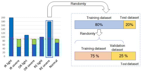
Figure 1.
Data organization: 80% of data were used to train 1D-CNN and 20% were used to test it. From training data, 75% were used to train the network, while 25% were used to validate it.
Having organized and balanced the three databases, CWRU, NSF-IMS and T-Y Wu databases were, respectively, used to (1) determine configuration parameters, (2) train a model and (3) generalize such a model.
2.3. 1D-CNN: Design and Configuration
The present model was inspired by applications of 1D-CNN in human pattern recognition and fault diagnosis systems [30,31]. This model, however, has fewer layers to reduce training time, and it only requires a single raw input (vibration signal).
The design process is presented in Figure 2 and was as follows. Firstly, the following parameters were adjusted: number of layers, quantity and size of filters for each layer, and training and optimization algorithms. Hyper parameters for the network were also adjusted. These were: number of signals per category, signal length, ratio training/testing, learning rate, learning training cycles (epochs) and training lot size (batch size). The recommended values are detailed in Table 3. Secondly, CNN structure was created as shown in Table 4. By determining the number of layers of the network model, it is possible to select both the quantity and dimensions of the filters of each convolutional layer. Table 5 presents the performance of each of the configurations that have been selected by adjusting a few options reported in the literature; in this case, the network structure in bold fonts was the best option. The internal structure and configuration of the Kernels filters are shown in Figure 3.
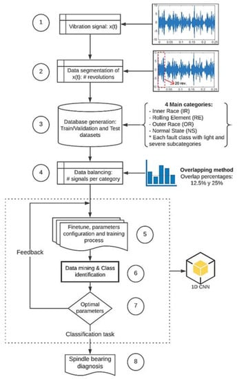
Figure 2.
Design and configuration of the proposed 1D-CNN method to detect spindle failures.
Table 3.
Hyper parameters configuration for the 1D-CNN.
Table 4.
1D-CNN structure.
Table 5.
Filter structure of the network.
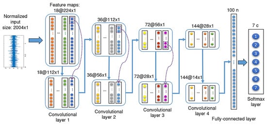
Figure 3.
Internal structure of 1D-CNN network.
For data mining, the network applies algorithms to automatically identify and select the most significant features from raw data. For this purpose, the convolution operation (Convolutive Layer) is applied to the input data, resulting in a vector with greater length and whose maximum clustering criterion (Max-Pooling Layer) is applied to extract the most representative features. The same procedure is repeated four times, but as can be seen in Table 4, the number of Kernels is increased for each Convolutive plus Max-Pooling set. This variation is performed to generate feature maps with the capacity to represent adequately the non-linearity of the signals. Figure 4 sequentially shows the generation of the first three values of a feature map by using a filter with a length of three samples and a sliding pass of one sample (stride). This operation is applied to each convolutional layer. The parameters that are regulated for this operation are the quantity and size of the filters (u), and the sliding factor of the window (stride).
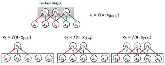
Figure 4.
Generation of feature maps in the convolutive layers.
The size of each feature vector is obtained by Equation (3). The configuration of the network requires only the calculation of map length of the last convolutional layer, since it is the input vector of the fully connected layer:
where flattenvector represents the size of the feature map, #filter indicates the number of filters of the convolutional layer, radio signals/cat indicates the amount of data by category, N represents the number of convolutional layers, and epochs is the number of training cycles. During each training cycle, new feature maps are generated and updated until the number of cycles that have been selected is completed. Two parameters are monitored in each iteration: the value of the loss function and the accuracy yielded by the network. The loss function of the 1D-CNN model is the crossed entropy between the probability distribution estimated by the Softmax layer and the probability distribution of the target class. The optimal learning parameters for the current model, in order to minimize the negative effect of random initialization of the weights and calculate the loss function, are calculated with the ADAM optimization stochastic algorithm in order to achieve greater efficiency during the training process.
For classification purposes, feature maps are used during the training for successive comparisons between the input signal and each map. At each comparison, each feature vector sweeps from the beginning to the end of the signal by means of a sliding window. The results of each comparison are kept as a vector. Each feature is a probability that the processed signal segment belongs to one of the bearing states.
For implementation, TensorFlow library for Python Deep Learning processing was used. The algorithm is illustrated in Figure 5. This consisted of importing libraries, entering training and testing data, and normalizing the signals before performing an internal random separation of the training set.
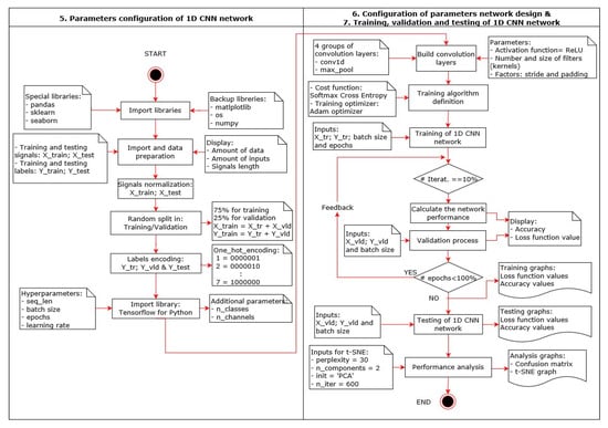
Figure 5.
1D-CNN network algorithm.
3. Results
The proposed 1D-CNN was evaluated in line with three parameters: (1) accuracy percentage, (2) confusion matrix and (3) t-distribution Stochastic Neighbor Embedding (t-SNE) algorithms. t-SNE refers to a 2D representation of the fully connected layer that allows for visual analysis of the classification performed by the network, using both the validation and testing sets.
The configuration-training-testing cycle described in previous section was run three times by (1) increasing the number of iterations, (2) varying the number of classes and (3) eliminating the most identifiable classes, so as to evaluate accuracy, generalization and versatility of 1D-CNN to identify spindle bearing failures. Results of the three evaluations are presented below.
3.1. Number of Iterations and Accuracy
The training performance after 2000 iterations was presented in Figure 6. As can be seen from the figure, moderate and severe RE failures were still misclassified. In addition, a comparison among different numbers of training cycles and learning rates was shown in Figure 7. As can be seen, the performance was not greatly modified by the number of training cycles, but the computing time was. It is shown that 50 epochs and a learning rate of 0.001 allows the network to achieve the highest performance for different numbers of classes.
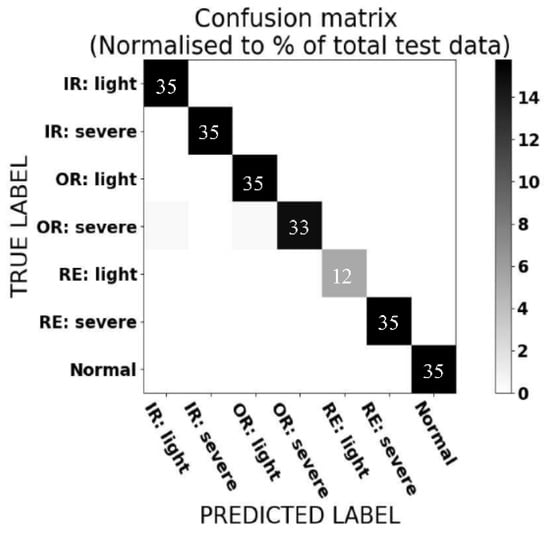
Figure 6.
Confusion matrix for the training process after 2000 iterations.
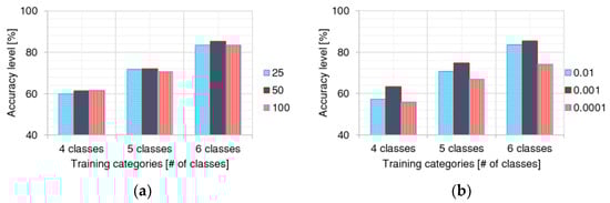
Figure 7.
Network performance at training in terms of number of epochs (a) and learning rates (b) for different classes.
In Figure 8, 1D-CNN training process is sequentially presented. From the figure, under- and over-fitting can be identified. For example, features are undistinguishable per class at iteration 10, but they are completely grouped at iteration 2000.
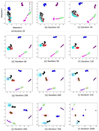
Figure 8.
Training process of the 1D-CNN: Comparison of different number of iterations, from 10 to 2000.
3.2. Number of Classes and Generalization
Table 6 shows 1D-CNN performance at different number of classes. In Table 6, it can be seen that the lowest accuracy (50%) is reached using four classes. In comparison, 80% accuracy is achieved using six classes. Four and five categories were selected for the training process because, in real applications, a huge number of unknown signals per second are obtained, and network performance needs to be at least acceptable under these training conditions.
Table 6.
1D-CNN performance using different number of classes.
The proposed 1D-CNN shows great generalization capability, since even when training with only four failure categories (Figure 9), the network can classify unknown faults into identifiable categories. For example, if the network is trained through the moderate IR failures, it correctly classifies severe IR failures. This indicates that the network has the ability to optimally learn different feature categories, as long as enough training data are provided. In essence, ID-CNN is achieving classification and clustering simultaneously.
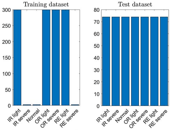
Figure 9.
Network behavior when training with four classes, but it successfully identifies seven classification categories.
3.3. Diffuse Classes and Specificity
To evaluate the system’s versatility is to classify the most diffuse classes. In Figure 10, the confusion matrix shows that IR failures are the easiest class to identify. Similarly, t-SNE algorithm indicates that severe and moderate IR failures are the easiest to identify. Therefore, all these classes were eliminated from the training database. By using the rest of the data, testing results are shown in Table 7.
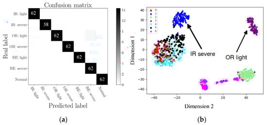
Figure 10.
Identification of difficult classification categories. (a) Confusion matrix of IMS, (b) t-SNE representation of IMS.
Table 7.
1D-CNN performance when only using classes that are difficult to classify.
4. Discussion
In the literature review, a clear trend since 2016 of using several feature extraction techniques, such as Fast Fourier Transform, Wavelet Package Energy Transform and Empirical Mode Decomposition (FFT, WPE and EMD), along with a classifier based on a DNN, is identified. Two-dimensional CNNs have been one of the most commonly used networks [32], but one-dimensional ones have not yet been applied to the same extent. One of the first investigations undertaken is presented in [30], where an accuracy of 100% is yielded with a processing time of 62 ms using a seven-layer model with the database reported in [22], requiring around 20,000 signals. The second investigation reported in [31] is a validated eight-layer model with around 20,000 data from the CWRU bearing database, reaching an accuracy of 99.77% with a very high capacity of noise robustness. A similar work is reported in [33], where a performance of 99.27% with 10,000 CWRU signals is achieved. Additionally, a comparable study is described in [34,35], where the accuracy rate is 100%, 99.76%, 99.77% and 99.57% with more than 177,000 CWRU signals, and 99% with 3500 CWRU signals, respectively. The third investigation reported in [36] is a deep auto-encoder method with fusing discriminant, where the IMS dataset is classified with an accuracy rate of 98.3%. Similar research is proposed in [37], where a methodology based on Deep Feature Learning for fault identification is applied. Each sample consists of 3000 data points; where a multi-domain feature calculation is applied, the accuracy is 99.8%. Finally, another method reported in [38] has above 99% accuracy rate using an optimized method of stacked variational denoising auto-encoder. In comparison, the proposed model has
- a lower number of layers (four convolutional, one fully connected, one Softmax),
- a reduced processing time of 8 ms per signal,
- an acceptable training time (~14 min) and
- a maximum performance of 99.64% with a standard deviation of 0.25%,
requiring an acceptable dataset (1904 signals) to reach maximum performance with three databases (see Table 8).
Table 8.
Comparison of the results obtained by the proposed model with other investigations.
The method of bearing failure diagnosis has been developed on the basis of feature learning approach. That is, the -CNN is divided into two main procedures: (1) feature extraction/selection that is undertaken by convolutional filters (Kernels) and (2) classification based on Softmax layer. The proposed model for bearing failure detection uses fewer layers and a different filter structure in comparison with similar networks. Furthermore, the network reaches a maximum accuracy of over 99% with three bearing databases and has a low average standard deviation (0.25%) for the multiple combinations and configurations in the training process. Generalizability and repeatability are achievable by selecting appropriate configuration parameters and structure.
DLNN presents high computational efficiency and achieves high performance accuracy with raw input signals. DLNNs have the capability to extract and classify features in a single structure, achieving a reliable diagnosis with low-cost computational processing in comparison with traditional feature extraction methods (WPE, EMD, HHT, etc.) in conjunction with typical classifiers.
In the analysis of the results, Case I refers to the database in [22] and is used to determine configuration parameters and train the model. Case II refers to the database in [24], and Case III refers to the database in [23]; both are used to test the performance, robustness and to generalize the proposed network. The model was also evaluated using Case II and III databases to determine configuration parameters and training process, reaching similar results to those achieved in Case I. The databases were selected because they combine different characteristics: shaft velocity, loads, severity level of failure and sampling frequency. One relevant aspect is that in Case I and III, the failures were generated using EDM method, while bearings of Case II ended their useful life naturally.
The robustness of the DL model has been tested from two points of view. First, according to a combination of operating conditions, the options used were: Case I and II with different constant shaft velocities (1720–2000 rpm) and Case III with variable velocities (300–750 rpm), as in a real operation. The three databases had several constant loads (0–3 hp), and three failure types (IR, OR and RE) were considered with two levels of severity (light and severe). Additionally, in Case I and II, the failures were introduced with EDM, but in Case III, the bearings ended their useful life naturally. The second point concerned dataset variations. Those were obtained by randomly suppressing one or several categories during training, showing that the network correctly learned from the most significant features that characterized severe and moderate bearing failures. In addition, the easiest identifiable bearing failures were discarded from the analysis in order to test robustness, and performance accuracy was not affected significantly.
5. Conclusions
The proposed model showed a great capacity to adapt to three types of configurations and three different databases, despite a training set with a smaller number of categories. The network still detected faults at early damage stages. Additionally, the low computational cost demonstrate DLNN’s suitability for real-time applications in industry.
In conclusion, the proposed 1D-CNN showed the following advantages:
- Higher accuracy was achieved by increasing the number of training iterations.
- Regardless of the number classes, the 1D-CNN allowed for differentiation of classes not even included as samples in the training stage.
- By eliminating the easiest identifiable classes, 1D-CNN yielded the highest accuracy in classifying more diffuse classes.
- Reduced processing time of around 8 ms per signal, demonstrating the possibility of real-time application.
As machinery failure and noise related to rotation speed are generated by vibration, the accurate and prompt detection of vibration signals based on 1D-CNN can lead to an identification of not only machinery failure, but also noise pollution. Additionally, noise pollution significantly alters human mood (e.g., stress, anxiety and loss of attention) and body functioning (e.g., heart and breathing rates, and blinks), which in turn affect work performance and life quality of nearby inhabitants, especially in harmonic frequencies that are not audible [39].
As future work, the developed model has been verified with vibration signals obtained by accelerometers. However, the use of convolutional network can be extended to using acoustic emission signals as system inputs. The proposed network model uses the backpropagation algorithm for training, and the criterion used to stop the process is the number of training cycles (epochs), so it is possible to implement a cross-validation algorithm to increase efficiency by stopping the process when the desired maximum performance is obtained. The processing speed and limited use of computational resources for the operation of the 1D CNN network mean that the applicability of this method is not only limited to the field of bearing fault detection, but can also be implemented in other important fields, such as medicine. The operational characteristics of the developed model meet the necessary requirements for applications that require real-time processing and being implemented in embedded devices, such as Raspberry Pi, Beaglebone, etc.
Author Contributions
Conceptualization, J.C.-S. and D.I.I.-Z.; methodology, D.I.I.-Z.; software, J.C.-S.; validation, L.M.A.-V. and J.C.-S.; formal analysis, D.I.I.-Z.; investigation, L.M.A.-V.; resources, J.C.-S.; data curation, J.C.-S.; writing—original draft preparation, D.I.I.-Z.; writing—review and editing, L.M.A.-V.; visualization, J.C.-S.; supervision, L.M.A.-V.; project administration, D.I.I.-Z.; funding acquisition, D.I.I.-Z. All authors have read and agreed to the published version of the manuscript.
Funding
This research was funded by Tecnologico de Monterrey.
Institutional Review Board Statement
Not applicable.
Informed Consent Statement
Not applicable.
Acknowledgments
The authors are deeply thankful for the support offered by Tecnologico de Monterrey and CONACYT.
Conflicts of Interest
The authors declare no conflict of interest.
References
- Lee, Y.O.; Jo, J.; Hwang, J. Application of deep neural network and generative adversarial network to industrial maintenance: A case study of induction motor fault detection. In Proceedings of the 2017 IEEE International Conference on Big Data (Big Data), Boston, MA, USA, 11–14 December 2017; pp. 3248–3253. [Google Scholar] [CrossRef]
- Li, X.; Ding, P.; Shi, X. Research on bearing fault detection based on convolution neural network. In Proceedings of the 2017 Chinese Automation Congress (CAC), Jinan, China, 20–22 October 2017; pp. 5130–5134. [Google Scholar] [CrossRef]
- Sharma, A.; Upadhyay, N.; Kankar, P.K.; Amarnath, M. Nonlinear dynamic investigations on rolling element bearings: A review. Adv. Mech. Eng. 2018, 10, 1687814018764148. [Google Scholar] [CrossRef]
- Ahmed, H.; Wong, M.L.D.; Nandi, A.K. Effects of deep neural network parameters on classification of bearing faults. In Proceedings of the IECON 2016—42nd Annual Conference of the IEEE Industrial Electronics Society, Florence, Italy, 24–27 October 2016; pp. 6329–6334. [Google Scholar] [CrossRef]
- Janssens, O.; Slavkovikj, V.; Vervisch, B.; Stockman, K.; Loccufier, M.; Verstockt, S.; Van de Walle, R.; Van Hoecke, S. Convolutional Neural Network Based Fault Detection for Rotating Machinery. J. Sound Vib. 2016, 377, 331–345. [Google Scholar] [CrossRef]
- Li, C.; Zhang, W.; Peng, G.; Liu, S. Bearing Fault Diagnosis Using Fully-Connected Winner-Take-All Autoencoder. IEEE Access 2017, 6, 6103–6115. [Google Scholar] [CrossRef]
- Peter, W.T.; Leung, J.T. Advanced system for automatically detecting faults occurring in bearings. In Fault Detection: Theory, Methods and Systems; Nova Science Publishers: New York, NY, USA, 2010; pp. 1–67. [Google Scholar]
- Zhao, R.; Yan, R.; Chen, Z.; Mao, K.; Wang, P.; Gao, R.X. Deep learning and its applications to machine health monitoring. Mech. Syst. Signal Process. 2019, 115, 213–237. [Google Scholar] [CrossRef]
- He, M.; He, D. Deep Learning Based Approach for Bearing Fault Diagnosis. IEEE Trans. Ind. Appl. 2017, 53, 3057–3065. [Google Scholar] [CrossRef]
- Shao, H.; Jiang, H.; Zhang, H.; Liang, T. Electric Locomotive Bearing Fault Diagnosis Using a Novel Convolutional Deep Belief Network. IEEE Trans. Ind. Electron. 2017, 65, 2727–2736. [Google Scholar] [CrossRef]
- Krizhevsky, A.; Sutskever, I.; Hinton, G.E. ImageNet Classification with Deep Convolutional Neural Networks. In Advances in Neural Information Processing Systems; Curran Associates Inc.: Red Hook, NY, USA, 2012; Volume 1, pp. 1097–1105. [Google Scholar]
- Zhao, G.; Zhang, G.; Ge, Q.; Liu, X. Research advances in fault diagnosis and prognostic based on deep learning. In Proceedings of the 2016 Prognostics and System Health Management Conference (PHM-Chengdu), Chengdu, China, 19–21 October 2016; pp. 1–6. [Google Scholar] [CrossRef]
- Schmidhuber, J. Deep Learning in Neural Networks: An Overview. Neural Netw. 2015, 61, 85–117. [Google Scholar] [CrossRef] [Green Version]
- Baker, M.A.; Holding, D.H. The Effects of Noise and Speech on Cognitive Task Performance. J. Gen. Psychol. 1993, 120, 339–355. [Google Scholar] [CrossRef]
- Cao, H.; Kang, T.; Chen, X. Noise analysis and sources identification in machine tool spindles. CIRP J. Manuf. Sci. Technol. 2019, 25, 26–35. [Google Scholar] [CrossRef]
- Verma, N.K.; Gupta, V.K.; Sharma, M.; Sevakula, R.K. Intelligent condition based monitoring of rotating machines using sparse auto-encoders. In Proceedings of the 2013 IEEE Conference on Prognostics and Health Management (PHM), Gaithersburg, MD, USA, 24–27 June 2013; pp. 1–7. [Google Scholar] [CrossRef]
- Lu, W.; Wang, X.; Yang, C.; Zhang, T. A Novel Feature Extraction Method using Deep Neural Network for Rolling Bearing Fault Diagnosis. In Proceedings of the 27th Chinese Control and Decision Conference (2015 CCDC), Qingdao, China, 23–25 May 2015. [Google Scholar]
- Qi, Y.; Shen, C.; Wang, D.; Shi, J.; Jiang, X.; Zhu, Z. Stacked Sparse Autoencoder-Based Deep Network for Fault Diagnosis of Rotating Machinery. IEEE Access 2017, 5, 15066–15079. [Google Scholar] [CrossRef]
- Chen, Z.; Li, Z. Research on fault diagnosis method of rotating machinery based on deep learning. In Proceedings of the 2017 Prognostics and System Health Management Conference (PHM-Harbin), Harbin, China, 9–12 July 2017; pp. 1–4. [Google Scholar] [CrossRef]
- Ding, X.; He, Q. Energy-Fluctuated Multiscale Feature Learning with Deep ConvNet for Intelligent Spindle Bearing Fault Diagnosis. IEEE Trans. Instrum. Meas. 2017, 66, 1926–1935. [Google Scholar] [CrossRef]
- Abdeljaber, O.; Avci, O.; Kiranyaz, S.; Gabbouj, M.; Inman, D.J. Real-time vibration-based structural damage detection using one-dimensional convolutional neural networks. J. Sound Vib. 2017, 388, 154–170. [Google Scholar] [CrossRef]
- Case Western Reserve University (CWRU). Bearing Data Center Website. 2017. Available online: https://csegroups.case.edu/bearingdatacenter/pages/welcome-case-western-reserve-university-bearing-data-center-website (accessed on 1 December 2020).
- Wu, T.Y.; Lai, C.H.; Liu, D.C. Defect diagnostics of roller bearing using instantaneous frequency normalization under fluctuant rotating speed. J. Mech. Sci. Technol. 2016, 30, 1037–1048. [Google Scholar] [CrossRef]
- NASA. NSF-IMS. Center for Intelligent Maintenance Systems: Bearing Data Set. 2018. Available online: https://ti.arc.nasa.gov/tech/dash/groups/pcoe/prognostic-data-repository/publications/#bearing (accessed on 1 December 2020).
- Qiu, H.; Lee, J.; Lin, J.; Yu, G. Wavelet filter-based weak signature detection method and its application on rolling element bearing prognostics. J. Sound Vib. 2006, 289, 1066–1090. [Google Scholar] [CrossRef]
- Lovrić, M.; Milanović, M.; Stamenković, M. Algoritmic Methods for Segmentation of Time Series: An Overview. J. Contemp. Econ. Bus. Issues 2014, 1, 31–53. [Google Scholar]
- Buda, M.; Maki, A.; Mazurowski, M.A. A systematic study of the class imbalance problem in convolutional neural networks. Neural Networks 2018, 106, 249–259. [Google Scholar] [CrossRef] [PubMed] [Green Version]
- García, V.; Alejo, R.; Sánchez, J.S.; Sotoca, J.M. Combined Effects of Class Imbalance and Class Overlap on Instance-Based Classification. In Proceedings of the International Conference on Intelligent Data Engineering and Automated Learning, Berlin, Germany, 20 September 2006. [Google Scholar]
- Dobbin, K.K.; Simon, R.M. Optimally splitting cases for training and testing high dimensional classifiers. BMC Med. Genom. 2011, 4, 31. [Google Scholar] [CrossRef] [Green Version]
- Zhang, W.; Peng, G.; Li, C.; Chen, Y.; Zhang, Z. A New Deep Learning Model for Fault Diagnosis with Good Anti-Noise and Domain Adaptation Ability on Raw Vibration Signals. Sensors 2017, 17, 425. [Google Scholar] [CrossRef]
- Zhang, W.; Zhang, F.; Chen, W.; Jiang, Y.; Song, D. Fault State Recognition of Rolling Bearing Based Fully Convolutional Network. Comput. Sci. Eng. 2018, 21, 55–63. [Google Scholar] [CrossRef]
- Wen, L.; Li, X.; Gao, L.; Zhang, Y. A New Convolutional Neural Network-Based Data-Driven Fault Diagnosis Method. IEEE Trans. Ind. Electron. 2017, 65, 5990–5998. [Google Scholar] [CrossRef]
- Zilong, Z.; Wei, Q. Intelligent fault diagnosis of rolling bearing using one-dimensional multi-scale deep convolutional neural network based health state classification. In Proceedings of the 2018 IEEE 15th International Conference on Networking, Sensing and Control (ICNSC), Zhuhai, China, 27–29 March 2018; pp. 1–6. [Google Scholar] [CrossRef]
- Yang, Y.; Fu, P.; He, Y. Bearing Fault Automatic Classification Based on Deep Learning. IEEE Access 2018, 6, 71540–71554. [Google Scholar] [CrossRef]
- Sun, J.; Yan, C.; Wen, J. Intelligent Bearing Fault Diagnosis Method Combining Compressed Data Acquisition and Deep Learning. IEEE Trans. Instrum. Meas. 2017, 67, 185–195. [Google Scholar] [CrossRef]
- Mao, W.; Feng, W.; Liu, Y.; Zhang, D.; Liang, X. A new deep auto-encoder method with fusing discriminant information for bearing fault diagnosis. Mech. Syst. Signal Process. 2020, 150, 107233. [Google Scholar] [CrossRef]
- Saucedo-Dorantes, J.J.; Arellano-Espitia, F.; Delgado-Prieto, M.; Osornio-Rios, R.A. Diagnosis Methodology Based on Deep Feature Learning for Fault Identification in Metallic, Hybrid and Ceramic Bearings. Sensors 2021, 21, 5832. [Google Scholar] [CrossRef]
- Yan, X.; Xu, Y.; She, D.; Zhang, W. Reliable Fault Diagnosis of Bearings Using an Optimized Stacked Variational Denoising Auto-Encoder. Entropy 2022, 24, 36. [Google Scholar] [CrossRef] [PubMed]
- Allahverdy, J.A.A. Non-auditory Effect of Noise Pollution and Its Risk on Human Brain Activity in Different Audio Frequency Using Electroencephalogram Complexity. Iran J. Public Health 2016, 45, 1332–1339. [Google Scholar] [PubMed]
Publisher’s Note: MDPI stays neutral with regard to jurisdictional claims in published maps and institutional affiliations. |
© 2022 by the authors. Licensee MDPI, Basel, Switzerland. This article is an open access article distributed under the terms and conditions of the Creative Commons Attribution (CC BY) license (https://creativecommons.org/licenses/by/4.0/).