COMMA: Propagating Complementary Multi-Level Aggregation Network for Polyp Segmentation

Abstract

Colonoscopy is an effective method for detecting polyps to prevent colon cancer. Existing studies have achieved satisfactory polyp detection performance by aggregating low-level boundary and high-level region information in convolutional neural networks (CNNs) for precise polyp segmentation in colonoscopy images. However, multi-level aggregation provides limited polyp segmentation owing to the distribution discrepancy that occurs when integrating different layer representations. To address this problem, previous studies have employed complementary low- and high- level representations. In contrast to existing methods, we focus on propagating complementary information such that the complementary low-level explicit boundary with abstracted high-level representations diminishes the discrepancy. This study proposes COMMA, which propagates complementary multi-level aggregation to reduce distribution discrepancies. COMMA comprises a complementary masking module (CMM) and a boundary propagation module (BPM) as a multi-decoder. The CMM masks the low-level boundary noises through the abstracted high-level representation and leverages the masked information at both levels. Similarly, the BPM incorporates the lowest- and highest-level representations to obtain explicit boundary information and propagates the boundary to the CMMs to improve polyp detection. CMMs can discriminate polyps more elaborately than prior CMMs based on boundary and complementary representations. Moreover, we propose a hybrid loss function to mitigate class imbalance and noisy annotations in polyp segmentation. To evaluate the COMMA performance, we conducted experiments on five benchmark datasets using five metrics. The results proved that the proposed network outperforms state-of-the-art methods in terms of all datasets. Specifically, COMMA improved mIoU performance by 0.043 on average for all datasets compared to the existing state-of-the-art methods.

1. Introduction

Colorectal cancer (CRC), which is one of the most common cancers globally, usually begins as a polyp in the colon mucosa, and approximately one-quarter of untreated polyps can develop into colon cancer [1]. Early polyp detection is a significant task in preventing CRC, and colonoscopy is used extensively as a standard polyp detection method [2,3,4]. Although colonoscopy is an effective method for detecting polyps at the early stages, polyp detection using colonoscopy images is a challenging task owing to the ambiguous image context. As polyps are usually small and their boundaries are low in contrast to their surroundings, polyps can easily be mistaken for wrinkles or other intestinal structures, leading to inaccurate segmentation and over-segmentation. Therefore, discrimination of the precise polyp region from an ambiguous context is critical for improving early polyp detection and preventing CRC.

Based on the need for elaborate segmentation, early studies utilized handcrafted features with a classifier [5,6]. However, the handcrafted approaches suffer from unsatisfactory performance because they cannot cover both intra- and inter-class variations [7]. Recent studies have proposed deep learning-based approaches, including fully convolutional networks (FCNs) [8] and U-Net [9]. Moreover, as alternative approach, Mask R-CNN [10] based models have also been proposed for precise polyp segmentation [11]. In contrast to existing CNN-based networks, PNS-Net [12] introduced a normalized self-attention network that dynamically operated the receptive field of the network. Along with the network architecture, a recent approach [13] considered excluding the effect of colors because polyp images are gathered under varying conditions. By alleviating discrepancies in color distribution, they improved the generalization performance of the network.

The U-Net comprises encoder-decoder structures that aggregate multiple encoder representations at the decoder to overcome the insufficient representations of the handcrafted approaches. Although the encoder-decoder structure improves the polyp segmentation performance, this structure exhibits a distribution discrepancy between the low- and high-level representations when aggregating multi-level features. Because the low-level representation contains sufficient boundary information with background noise, whereas the high-level feature presents abstracted region information [14,15,16]. To overcome the drawbacks of both representations, each level requires the elimination of noise and an emphasis on boundary information. Without the denoising and refining fine information, the multi-level aggregation discrepancy occurs and it generates rough boundaries with noise in the prediction map, which limits the model performance. To reduce this discrepancy, U-Net++ [17] proposed multiple convolution layers on the skip pathways between the encoder and decoder features. A previous study [18] improved on existing U-Net++-based architecture by applying conditional random field and test-time augmentation to the ResUNet++ [19] for precise polyp segmentation. Focusing more on the multi-level aggregation problem, previous studies [20,21] organized the network including selective feature extraction and aggregation using multiple kernel sizes. In addition, Enhanced U-Net [22] introduced attention modules designed to extract distinct features from the highest-level representation with different patch sizes and to refine the encoder features by utilizing the distinct features. Similarly, SANet [13] proposed fusing both low- and high-level representations to detect fine polyps by excluding background noise in low-level representations with abstracted high-level information. These existing studies contributed to diminishing the multi-level distribution discrepancy; however, they did not propagate complementary low- and high-level aggregation to decoder structure to clarify polyp representation. Based on the lack of research on the propagation of complementary multi-level aggregated information, we studied the relationship between low- and high-level representations and focused on the propagation of complementary information.

Another approach is the use of boundary information to compensate for insufficient polyp representation. Psi-Net [23] addressed a joint training strategy using polyp region and boundary detection tasks. Moreover, SFANet [20] incorporated boundary-sensitive loss with boundary deep supervision maps [24] to detect polyp boundaries more elaborately. In terms of boundary refinement, MSBNet [25] utilized a low-level representation with a Gaussian kernel to enhance boundary information at the highest representation. Another study [26] organized multiple boundary attention modules designed to discriminate boundary information using encoder and decoder representations adjacent to each other at each decoder. In PraNet [27], which improved the model efficiency and outperformed existing studies, a parallel reverse attention method with partial decoders was employed to incorporate the polyp area and boundary features [15,28]. Although PraNet considered the region and boundaries, the reverse attention method could not sufficiently discriminate the boundary from the background. Because the boundary is obtained by aggregating the high-level encoder outputs, which present the abstracted region information, the reversed region contains insufficient boundaries compared to low-level outputs. In previous studies, the explicit boundary information can be propagated across the decoders to detect the polyp boundaries more elaborately, although the boundary was either used independently in a single decoder or not proliferated. Therefore, we focused on propagating the explicit boundary by employing a multi-decoder structure.

In medical image segmentation tasks, binary cross entropy (BCE) and IoU losses are commonly used to deal with local and global structural awareness. The BCE and IoU losses cause a class imbalance problem because they treat all pixels with equal importance. To reduce this problem, weighted BCE (wBCE) and IoU (wIoU) losses have been proposed in previous studies on salient object detection tasks [29]. In polyp segmentation, PraNet [27] demonstrated state-of-the-art performance by adopting wBCE and wIoU losses. In addition, we consider an L1 distance loss, which can handle noisy annotations [30,31] often encountered in segmentation tasks. Thus, we combine the wBCE, wIoU, and L1 loss functions to treat class imbalance and noisy label problems.

This study proposes a propagating complementary multi-level aggregation network (COMMA), which comprises a complementary masking module (CMM) and boundary propagation module (BPM) as the multi-decoder structure. The CMM clarifies the boundary noise in the low-level through the abstracted high-level representation and propagates the refined information to another decoder. The BPM generates an explicit boundary by masking the lowest-level representation through the highest-level outputs. The boundary is propagated to the CMMs in the next decoder to enhance the segmentation performance. We also propose a hybrid loss function that allows the network to learn robustly on noisy labels and assigns different importance to each pixel.

The main contributions of this study are as follows: First, we propose complementary multi-level aggregation, which contributes to reducing the multi-level distribution discrepancy by applying the abstracted high-level representation as a mask to the low-level boundary noises and propagating the complementary information. Second, the explicit boundary propagation for the multi-decoder discriminates polyps in an ambiguous context and enhances the segmentation performance. Third, we design a hybrid loss function consisting of weighted BCE, weighted IoU, and L1 distance loss. The hybrid loss function enables the model to focus on relatively important pixels and to be robust against noisy annotations. Fourth, as a novel network, COMMA achieves state-of-the-art performance with a significant improvement in the generalization performance.

The remainder of this study is as follows. Section 2 explains the proposed COMMA architecture for polyp segmentation. Section 3 describes the experimental setup and obtained results. Section 4 presents a discussion of the proposed method. Finally, Section 5 concludes this study and outlines future works.

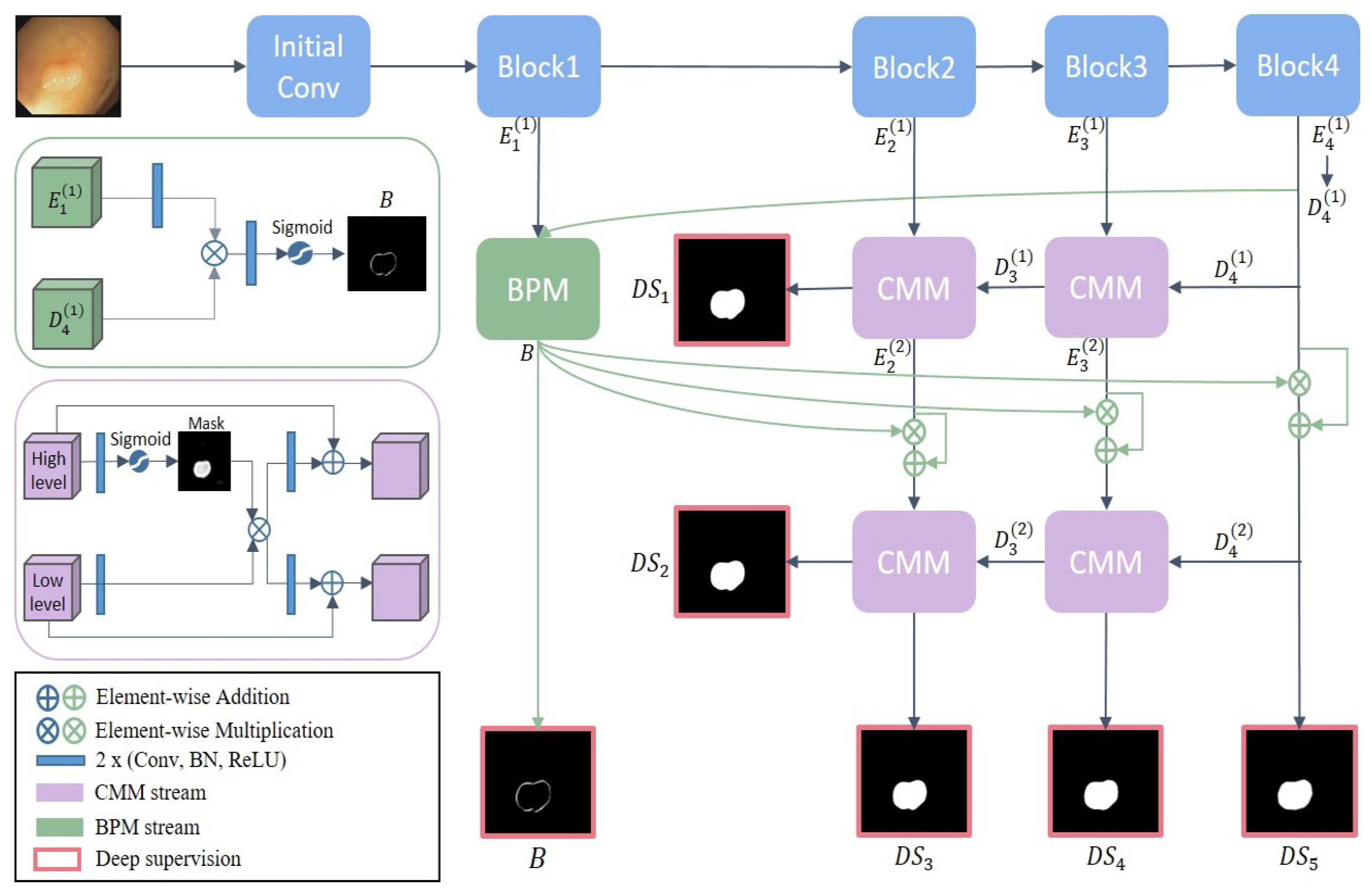
2. Materials and Methods

In this section, we present COMMA, which is designed to reduce the multi-level distribution discrepancy by propagating both refined levels and explicit boundary information. Figure 1 represents the proposed COMMA architecture, consisting of an encoder block and a decoder block containing the CMM and BPM. The encoder blocks consist of four stages based on ResNet [32] and Res2Net [33], and the CMM extracts a complementary representation by aggregating the encoder output and the previous decoder output. The BPM in the decoder combines the highest- and lowest-level features to extract explicit boundary information. Furthermore, to proliferate distinct information, we employ multi-decoder structures consisting of CMMs and BPM.

2.1. Complementary Masking Module

Based on the relationship between the relatively low- and high-level representations, the CMM masks the background noise at the low-level representation through the abstracted high-level representation. After obtaining the denoised representation, we propagate the complementary information to the decoder representation and the next decoder. Here, we denote the i-th encoder block representation $E_i^{\left(j\right)}$ in the j-th skip connection path, where $i\in \{1,2,3,4\}$ and $j\in \{1,2\}$. $D_i^{\left(j\right)}$ indicates the i-th decoder block representation in the j-th decoder, where $i\in \{3,4\}$ and $j\in \{1,2\}$. In the CMM, the encoder output $E_i^{\left(j\right)}\in {\mathbb{R}}^{C_i\times H_i\times W_i}$ is masked by the decoder output $D_{i+1}^{\left(j\right)}\in {\mathbb{R}}^{C_{i+1}\times H_{i+1}\times W_{i+1}}$, as follows:

$$\begin{array}{c}mask=\sigma (\mathcal{F}(Up(D_{i+1}^{\left(j\right)})))\in {\mathbb{R}}^{1\times H_i\times W_i}\\ \mathcal{C}=\mathcal{F}(E_i^{\left(j\right)})\otimes mask\end{array}$$

(1)

Here, $Up(·)$ and $\mathcal{F}(·)$ indicate the bilinear upsampling and post-activated convolutional operations (i.e., Conv2D-Batch normalization-ReLU) [34], respectively. We apply a dual post-activation convolutional operation to $E_4^{\left(1\right)}$ for the first decoder representation $D_4^{\left(1\right)}$. To exclude the background noise, we apply $\mathcal{F}(·)$ to the upsampled decoder representation $Up(D_{i+1}^{\left(j\right)})$ to obtain the $mask$ that high-level representation is channel-wise aggregated. Subsequently, we employ a sigmoid function $\sigma$ to discriminate the mask information and eliminate the background noise in $E_i^{\left(j\right)}$ through $mask$. Following the masking, a post-activated convolutional operation is applied to complementary representation $\mathcal{C}$ to refine the features in each path of low- and high-level. These features are fused with the original CMM input features ($E_i^{\left(j\right)}$ and $D_{i+1}^{\left(j\right)}$) to propagate the next CMM and decoder as follows:

$$\begin{array}{c}{E}_i^{\left(j\right)}=\mathcal{F}\left(\mathcal{C}\right)+E_i^{\left(j\right)},D_i^{\left(j\right)}=\mathcal{F}\left(\mathcal{C}\right)+Up(D_{i+1}^{\left(j\right)})\end{array}$$

(2)

For an efficient computation, we include two CMMs in a single decoder. Then, to progressively improve and propagate the complementarity of the output propagated to the next decoder CMM, we designed a cascading multi-decoder structure. We describe an experiment in Section 3.4.1 in which we investigated the effects of progressive improvement in complementarity. Finally, we obtain five deep supervision maps [24]: two decoder path outputs ($D{S}_1$ and $D{S}_2$) and three skip-connected path outputs ($D{S}_3$, $D{S}_4$, and $D{S}_5$). Each deep supervision map is upsampled to the ground truth size to compute the model loss.

2.2. Boundary Propagation Module

Explicit boundary information contributes to a more elaborate discrimination of polyps in ambiguous contexts. Existing studies [25,26] generated edge information by ensembling both low- and relatively high-level representations. They only utilized this information to refine the highest-level feature or adjacent pair of encoder-decoder outputs, rather than the entire network. In contrast to existing methods, the BPM is designed not only to detect explicit boundary information but also to propagate the boundary to complementary multi-level features by incorporating the lowest- and highest-level representations. Although both levels exhibit a large distribution discrepancy, we overcome the discrepancy with a property of each level to obtain a detailed boundary. The low-level encoder output contains sufficient boundary information including background noise; in contrast, the high-level output contains abstracted position information such that it exhibits ambiguous boundaries [14,15,16]. Based on these properties, we consider both the lowest and highest levels to maximize boundary detection performance. To verify the effectiveness of this adoption, we conducted an ablation study related on the representation level for boundary generation in Section 4.2.

We denoise the boundary noise at the lowest-level $E_1^{\left(1\right)}$ through the highest-level representation $D_4^{\left(1\right)}$ to obtain a high-quality boundary, as follows:

$$\begin{array}{c}X=\mathcal{F}(E_1^{\left(1\right)})\otimes Up(D_4^{\left(1\right)})\\ B=\sigma (\mathcal{F}\left(X\right))\end{array}$$

(3)

A convolutional operation $\mathcal{F}(·)$ removing background noise [35,36] is applied to $E_1^{\left(1\right)}$. $D_4^{\left(1\right)}$ for the effective aggregation of two different levels is directly rescaled to the same size as $E_1^{\left(1\right)}$ by the bilinear upsampling $Up(·)$. Subsequently, we refine the fused feature X using $\mathcal{F}(·)$ and employ a sigmoid function to discriminate the boundary representation B. After generating the explicit boundary B, the BPM propagates downsampled B to complementary representations $E_i^{\left(2\right)}$, which are the CMM outputs of the first decoder, to clarify the fine information, as follows:

$$\begin{array}{c}{E}_i^{\left(2\right)}=E_i^{\left(2\right)}\otimes Down\left(B\right)+E_i^{\left(2\right)},wherei=2,3,4\end{array}$$

(4)

Here, $Down(·)$ indicates bilinear downsampling to the same size as $E_i^{\left(2\right)}$. We emphasize boundary information in $E_i^{\left(2\right)}$ using resized B to each $E_i^{\left(2\right)}$. By enhancing the fine features at each $E_i^{\left(2\right)}$, which is the input of the second decoder, the second decoder can more easily detect ambiguous polyps compared to the first. That is, boundary propagation is capable of learning a robust network against ambiguous edge information. To verify the effectiveness of boundary propagation, we present experimental results depending on the BPM application in Section 4.1. Finally, as demonstrated in existing studies [20,23,37], we generate a boundary ground truth $G{T}_B$ to improve the boundary detection performance. To support the explainability of the module, we visualize feature maps corresponding to the BPM application state in Section 4.3.

2.3. Hybrid Loss Function

We employ hybrid loss to constrain the area, boundary, and noisy annotations in the loss function as follows: $\mathcal{L}=\alpha *{\mathcal{L}}_{BCE}^w+\beta *{\mathcal{L}}_{IoU}^w+\gamma *{\mathcal{L}}_{L1}$. In medical image segmentation tasks, binary cross entropy (BCE) and IoU losses are adopted extensively to impose local and global constraints. The BCE and IoU losses consider all pixels to make equal contributions [29]. That is, because colonoscopy images contain more background than polyp regions, a class imbalance problem can occur. To prevent this imbalance, we utilize the weighted BCE (wBCE) and IoU (wIoU) losses, which focus on hard pixels, as demonstrated in previous study [29]. The weighted loss uses $\lambda$ to calculate the importance of each pixel, and ${\lambda }_{ij}$ is calculated as follows:

$$\begin{array}{c}{\lambda }_{ij}=\left|\frac{{\displaystyle \sum _{h,w\in A_{ij}}}{y}_{h,w}}{{\displaystyle \sum _{h,w\in A_{ij}}}1}-y_{ij}\right|\end{array}$$

(5)

Here, $A_{ij}$ refers to the area surrounding the target pixel $(i,j)$. The value of ${\lambda }_{ij}$ is larger when it is placed at the boundaries of the polyp compared to the center of the polyp. Thus, the weighted loss allows the network to focus on the boundary regions. For example, wBCE loss is given by Equation (6). Here, y and $\widehat{y}$ indicate the ground truth and prediction of each pixel, respectively. The notation $c\in \{0,1\}$ refers to binary classes. $\gamma$ is a hyper-parameter and is set to 5 as in previous study [29]. In wBCE, the importance of each pixel is assigned using weight ${\lambda }_{ij}$. As a result, the network can focus more on the local structures at the boundaries than using the BCE.

$$\begin{array}{c}{\mathcal{L}}_{BCE}^w=-\frac{{\displaystyle \sum _i^H}{\displaystyle \sum _j^W}(1+\gamma ·{\lambda }_{ij}){\displaystyle \sum _{c=0}^1}(y_{c}log\left({\widehat{y}}_c\right)+(1-y_c)log(1-{\widehat{y}}_c))}{{\displaystyle \sum _i^H}{\displaystyle \sum _j^W}(1+\gamma ·{\lambda }_{ij})}\end{array}$$

(6)

In contrast, the wIoU loss detects the global structure of the polyp rather than individual pixels based on the pixel importance ${\lambda }_{ij}$.

$$\begin{array}{c}{\mathcal{L}}_{IoU}^w=1-\frac{{\displaystyle \sum _i^H}{\displaystyle \sum _j^W}\left(y_{ij}{\widehat{y}}_{ij}\right)(1+\gamma ·{\lambda }_{ij})}{{\displaystyle \sum _i^H}{\displaystyle \sum _j^W}(y_{ij}+{\widehat{y}}_{ij}-y_{ij}{\widehat{y}}_{ij})(1+\gamma ·{\lambda }_{ij})}\end{array}$$

(7)

Moreover, we consider the L1 distance loss to be robust to noisy labels [30,31], which often occurs when annotating in segmentation tasks, so that the model converges robustly and reliably on noisy annotations.

$$\begin{array}{c}{\mathcal{L}}_{L1}=\frac{1}{H\times W}{\displaystyle \sum _i^H}{\displaystyle \sum _j^W}|y_{ij}-{\widehat{y}}_{ij}|\end{array}$$

(8)

We provide the ablation studies exploring different combinations by calibrating the loss weights (i.e., $\alpha$, $\beta$, and $\gamma$) in Section 4.4.2. Moreover, existing study [27] revealed that explicitly using the dependency of both region and boundary causes an overfitting problem; however, we avoid this issue by applying independent boundary loss and data augmentations. Based on the hybrid loss, the final loss is calculated using the deep supervision maps as follows:

$$\begin{array}{c}{\mathcal{L}}_{final}={\displaystyle \sum _{i=1}^5}\mathcal{L}(GT,D{S}_i)+\mathcal{L}(G{T}_B,B)\end{array}$$

(9)

As we combine three different loss functions, we investigate the effectiveness of each and their contributions to the performance improvement in Section 4.4.

3. Results

In this section, we demonstrate the five benchmark datasets, five evaluation metrics, and experimental setups used for as well as the results of evaluating COMMA performance compared to existing methods.

3.1. Dataset

We validated the proposed COMMA using five datasets. Kvasir-SEG [38] is the largest dataset, containing 1000 challenging images for polyp segmentation. We divided Kvasir into 80%, 10%, and 10% for the training, validation, and testing images, respectively, following the experimental settings of the existing study [27]. CVC-ClinicDB (CVC-612) [39] contains 612 images in which the boundaries are low in contrast to their surroundings. In the same manner, we used 550 images (90%) for training and validation and 62 images (10%) for testing. To enable a fair comparison, all test sets were equivalent to those in previous study [27]. CVC-ColonDB [40], ETIS [41], and EndoScene (CVC-T, CVC-300) [42] were used to evaluate the generalization performance, because these small datasets contain 380, 196, and 60 images, respectively.

3.2. Experimental Setup

3.2.1. Evaluation Metrics

To validate the performance of the proposed model, we employed the mean Dice and mean IoU metrics, which are widely used in medical image segmentation tasks. Furthermore, we evaluated three additional metrics (i.e., $S_m$, $E_m$, and MAE) that are commonly used in salient object detection tasks [15,37,43]. The S-measure [44], which evaluates structural similarities, is calculated as follows: $S_m=\alpha \times S_o+(1-\alpha )\times S_r$. $S_o$ and $S_r$ indicate the object- and region-aware structural similarity, respectively, and we set $\alpha =0.5$. The E-measure [45] considers the difference between the prediction and ground truth in terms of both the global and pixel levels. The MAE is computed by the average of the pixel-wise absolute values.

3.2.2. Implementation Details

For a fair comparison, we followed the experimental settings of the existing study [27]. The study concatenated both Kvasir and CVC-ClinicDB datasets. Afterward, they separated training, validation, and test sets to 80%:10%:10%, respectively. We applied a flip, blur, brightness, and distortion series for data augmentation to improve the model generalization effect. An Adam optimizer with a learning rate of 1 $\times {10}^{-4}$ and weight decay of 1 $\times {10}^{-4}$ was employed. We calibrated the learning rate with an increment of 0.1, by monitoring the validation loss if the validation loss did not reduce after 10 epochs. Moreover, an early stopping strategy was applied if the validation loss did not decrease for 20 epochs. We set the batch size to 32 and the maximum epochs to 200, and the input images were resized to 384 × 384. ResNet-50 [32] and Res2Net-50 [33] were employed as backbone networks by initializing the pre-trained on ImageNet datasets. We used a AMD-RYZEN R9 5900X CPU and single RTX 3090 GPU in this experiment, and COMMA was implemented using the PyTorch framework.

3.3. Experimental Results

3.3.1. Comparison with State-of-the-Art Methods

We compared the proposed network with eight existing methods [9,17,19,20,22,25,27,46]. For unbiased comparison, we compared the proposed method to the state-of-the- arts [9,17,19,20,22,25,27,46] using the prediction maps pre-computed by the existing study [27] and the scores obtained from the published papers [19,22,25]. As demonstrated in

Table 1. Comparison of COMMA performance with existing state-of-the-art methods on CVC-ClinicDB and Kvasir datasets, where n/a indicates an inaccessible prediction map, and * and † indicate that the ResNet and Res2Net backbone encoders were employed, respectively.

Model	CVC-ClinicDB					Kvasir
	mDice	mIoU	${\mathit{S}}_{\mathit{m}}$	${\mathit{E}}_{\mathit{m}}$	MAE	mDice	mIoU	${\mathit{S}}_{\mathit{m}}$	${\mathit{E}}_{\mathit{m}}$	MAE
U-Net [9]	0.823	0.760	0.890	0.953	0.019	0.818	0.750	0.858	0.893	0.055
U-Net++ [17]	0.794	0.733	0.873	0.931	0.022	0.821	0.747	0.862	0.909	0.048
ResUNet-mod [46]	0.779	0.455	n/a	n/a	n/a	0.791	0.429	n/a	n/a	n/a
ResUNet++ [19]	0.796	0.796	n/a	n/a	n/a	0.813	0.793	n/a	n/a	n/a
SFA [20]	0.702	0.611	0.793	0.885	0.042	0.725	0.614	0.781	0.849	0.075
PraNet ${}^{†}$ [27]	0.899	0.853	0.937	0.979	0.009	0.897	0.844	0.915	0.948	0.030
COMMA *	0.916	0.871	0.947	0.979	0.008	0.904	0.860	0.925	0.963	0.024
COMMA ${}^{†}$	0.933	0.891	0.956	0.985	0.007	0.901	0.852	0.919	0.951	0.027

, COMMA achieved state-of-the-art performance on five evaluation metrics compared to previous methods. ResNet-50, as a backbone encoder, showed outstanding performance on the CVC-ClinicDB, whereas Res2Net50 outperformed the existing methods on the Kvasir dataset. In terms of the generalization performance, as shown in

Table 2. Comparison of COMMA generalization performance with state-of-the-art methods on CVC-ColonDB, ETIS, and CVC-T datasets. * and † indicate that the ResNet and Res2Net backbone encoders were employed, respectively.

Dataset	Model	mDice	mIoU	${\mathit{S}}_{\mathit{m}}$	${\mathit{E}}_{\mathit{m}}$	MAE
ColonDB	U-Net [9]	0.504	0.440	0.710	0.781	0.059
	U-Net++ [17]	0.482	0.412	0.693	0.764	0.061
	SFA [20]	0.457	0.341	0.628	0.753	0.094
	PraNet ${}^{†}$ [27]	0.711	0.644	0.820	0.872	0.043
	E: U-Net [22]	0.740	0.663	-	-	-
	MSBNet [25]	0.741	-	0.826	0.875	0.040
	COMMA *	0.712	0.645	0.823	0.864	0.045
	COMMA ${}^{†}$	0.754	0.689	0.849	0.897	0.037
ETIS	U-Net [9]	0.399	0.340	0.684	0.740	0.036
	U-Net++ [17]	0.401	0.348	0.683	0.776	0.035
	SFA [20]	0.298	0.221	0.557	0.632	0.109
	PraNet ${}^{†}$ [27]	0.628	0.571	0.794	0.841	0.031
	E: U-Net [22]	0.651	0.582	-	-	-
	MSBNet [25]	0.606	-	0.772	0.841	0.023
	COMMA *	0.709	0.643	0.845	0.887	0.018
	COMMA ${}^{†}$	0.711	0.648	0.844	0.887	0.015
CVC-T	U-Net [9]	0.711	0.631	0.843	0.875	0.022
	U-Net++ [17]	0.708	0.629	0.839	0.898	0.018
	SFA [20]	0.468	0.334	0.641	0.817	0.065
	PraNet ${}^{†}$ [27]	0.871	0.801	0.925	0.972	0.010
	E: U-Net [22]	0.886	0.813	-	-	-
	MSBNet [25]	0.866	-	0.917	0.966	0.010
	COMMA *	0.871	0.801	0.924	0.980	0.011
	COMMA ${}^{†}$	0.906	0.843	0.945	0.988	0.006

, COMMA exhibited significant improvement on the three unseen datasets (i.e., CVC-ColonDB, ETIS, and CVC-T). Compared to the state-of-the-art method, PraNet (32.55 M), which is the previous outstanding approach, COMMA required fewer learning parameters (31.1 M), but the segmentation performance was improved. As we obtained network robustness by leveraging the explicit boundary propagation and large samples with data augmentation, COMMA could detect unknown polyps more elaborately.

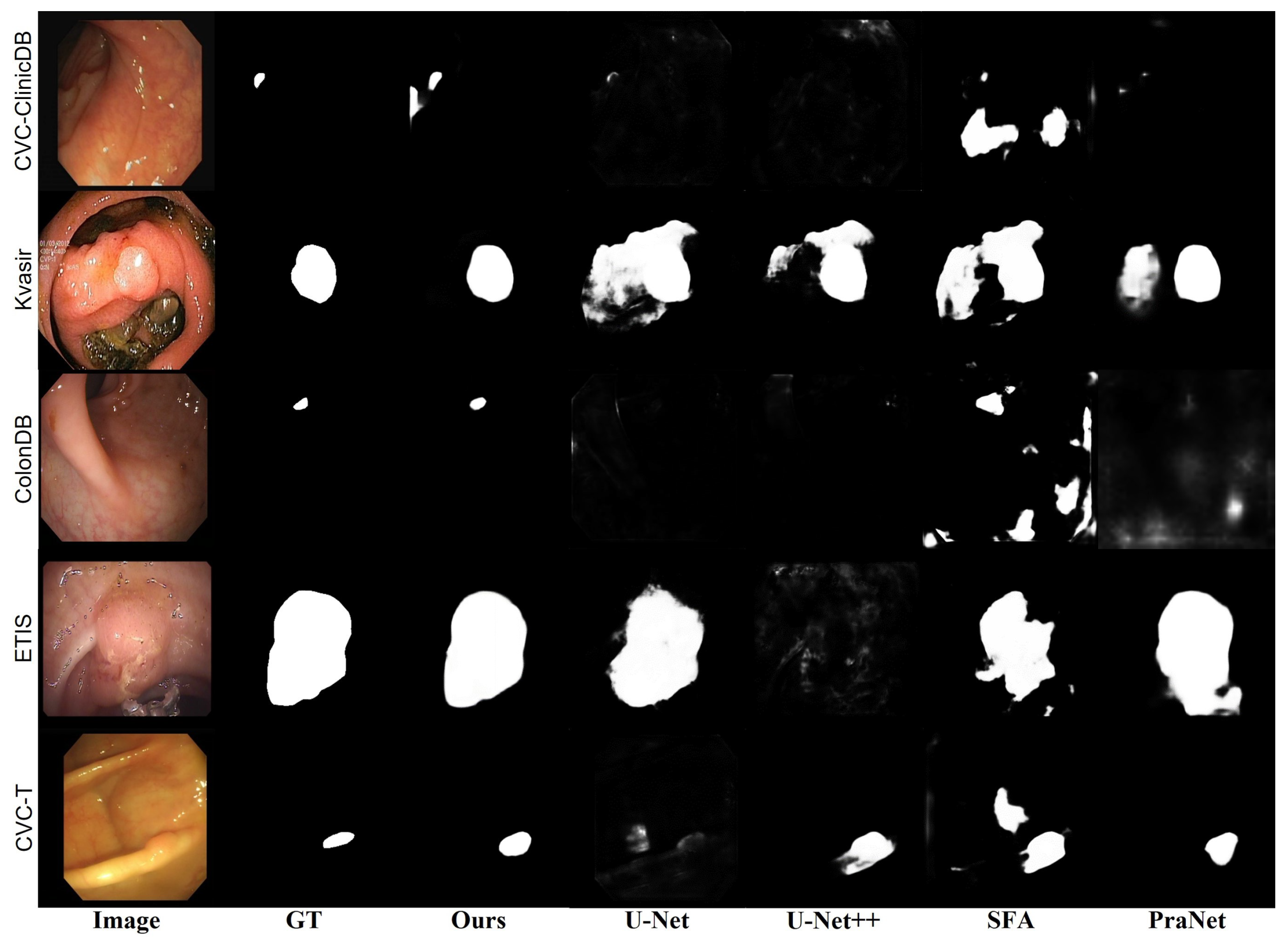
3.3.2. Qualitative Comparison

As illustrated in Figure 2, we randomly sampled polyp images from each dataset to validate the COMMA performance through the prediction maps. The images in the first and third rows were necessarily difficult cases because they included small polyps in the low-brightness areas. Although U-Net, U-Net++, and PraNet did not predict polyp areas, the proposed method detected polyp areas with some noise. This may be helpful to clinicians performing colonoscopy by improving polyp segmentation, where reducing false negatives is important. The images in the second and fifth rows show a low color contrast with the surrounding tissue. As as result of similar issues, previous methods tend to overestimate the surrounding tissue as a polyp, whereas the proposed method accurately predicted polyps. In the fourth-row image, which contains a large-scale polyp, the existing methods could not detect polyp regions with boundaries elaborately; in contrast, the proposed method was able to discriminate the polyp regions and boundaries. As a result, COMMA segregated the polyps in low-contrast and varied-size contexts by leveraging explicit boundaries and complementary representation.

3.3.3. Inference Analysis

As listed in

Table 3. Inference analysis of four datasets in the same environment. FPS refers to the number of frames processed per second.

Models	Batch.	#Params	CVC-ClinicDB			Kvasir			ColonDB			ETIS			Mean FPS
			mDice	MAE	FPS	mDice	MAE	FPS	mDice	MAE	FPS	mDice	MAE	FPS
PraNet	1	32.55 M	0.899	0.009	32.99	0.897	0.030	31.71	0.711	0.043	37.10	0.628	0.031	19.56	30.34
COMMA	1	31.10 M	0.933	0.007	42.32	0.901	0.027	31.90	0.754	0.037	51.96	0.711	0.015	42.31	42.12
COMMA	8	31.10 M	0.933	0.007	71.30	0.901	0.027	46.47	0.754	0.037	110.00	0.711	0.015	71.07	74.70

, we compared the proposed method with the PraNet with respect to inference times. All execution times were measured under the model declaration and data I/O times. To provide an unbiased comparison, we used the code and hyper-parameters released by the authors [27]. For the same batch size, COMMA required fewer parameters, was 1.39× faster, and performed significantly better than PraNet. Furthermore, we changed the batch size to eight and found that the average FPS was 74.70, which is sufficient for real-time operation.

3.4. Further Experiments

3.4.1. Effectiveness of Multi-Decoder Structure

We also conducted experiments on the effectiveness of the number of decoders in multi-decoder structures. As listed in

Table 4. Comparison of COMMA performance based on the decoder structures.

Dataset	#Decoder (d)	#Params	mDice	mIoU	${\mathit{S}}_{\mathit{m}}$	${\mathit{E}}_{\mathit{m}}$	MAE
CVC-ClinicDB	1	28.43 M	0.919	0.875	0.944	0.978	0.0072
	2	31.10 M	0.933	0.891	0.956	0.985	0.0066
	3	33.76 M	0.925	0.882	0.945	0.981	0.0074
	4	36.42 M	0.931	0.889	0.953	0.982	0.0068
	5	39.09 M	0.921	0.878	0.950	0.979	0.0074
Kvasir	1	28.43 M	0.870	0.823	0.898	0.920	0.032
	2	31.10 M	0.901	0.852	0.919	0.951	0.027
	3	33.76 M	0.898	0.849	0.919	0.953	0.028
	4	36.42 M	0.897	0.848	0.918	0.957	0.028
	5	39.09 M	0.901	0.851	0.919	0.950	0.027
ColonDB	1	28.43 M	0.701	0.665	0.817	0.844	0.051
	2	31.10 M	0.754	0.689	0.849	0.897	0.037
	3	33.76 M	0.762	0.697	0.852	0.874	0.039
	4	36.42 M	0.756	0.689	0.850	0.875	0.035
	5	39.09 M	0.753	0.689	0.846	0.876	0.039
ETIS	1	28.43 M	0.677	0.621	0.831	0.880	0.0160
	2	31.10 M	0.711	0.648	0.844	0.887	0.0151
	3	33.76 M	0.708	0.644	0.844	0.878	0.0176
	4	36.42 M	0.711	0.649	0.844	0.893	0.0164
	5	39.09 M	0.694	0.633	0.836	0.874	0.0167
CVC-T	1	28.43 M	0.850	0.793	0.894	0.957	0.012
	2	31.10 M	0.906	0.843	0.945	0.988	0.006
	3	33.76 M	0.892	0.826	0.935	0.987	0.007
	4	36.42 M	0.870	0.803	0.927	0.964	0.008
	5	39.09 M	0.888	0.822	0.936	0.977	0.009

, we observed that the multi-decoder structures are more effective in obtaining detailed polyp regions than the single-decoder structure. In the multi-decoder structures, while all the number of decoders from two to five are effective, two decoders achieve slightly better performance with fewer learning parameters, justifying this selection as the basis of the number of decoders.

3.4.2. Individual Learning

In the experiments, we trained a total dataset that merged CVC-ClinicDB and Kvasir datasets to obtain the leverage effect of a large distribution. We compared the results of training using CVC-ClinicDB and Kvasir as training datasets to investigate whether the benefits of the total dataset help to improve performance. As listed in

Table 5. Leverage effectiveness in large samples. † and * indicate that CVC-ClinicDB and Kvasir were used as training datasets, respectively.

Dataset	Model	mDice	mIoU	${\mathit{S}}_{\mathit{m}}$	${\mathit{E}}_{\mathit{m}}$	MAE
CVC-ClinicDB	PraNet	0.899	0.853	0.937	0.979	0.009
	COMMA ${}^{†}$	0.919	0.877	0.948	0.984	0.007
	COMMA	0.933	0.891	0.956	0.985	0.007
Kvasir	PraNet	0.897	0.844	0.915	0.948	0.030
	COMMA *	0.913	0.867	0.929	0.965	0.024
	COMMA	0.901	0.852	0.919	0.951	0.027
ColonDB	PraNet	0.711	0.644	0.820	0.872	0.043
	COMMA ${}^{†}$	0.757	0.690	0.849	0.893	0.038
	COMMA *	0.676	0.609	0.803	0.858	0.045
	COMMA	0.754	0.689	0.849	0.897	0.037
ETIS	PraNet	0.628	0.571	0.794	0.841	0.031
	COMMA ${}^{†}$	0.671	0.593	0.820	0.830	0.036
	COMMA *	0.689	0.616	0.829	0.863	0.023
	COMMA	0.711	0.648	0.844	0.887	0.015
CVC-T	PraNet	0.871	0.801	0.925	0.972	0.010
	COMMA ${}^{†}$	0.850	0.785	0.914	0.960	0.014
	COMMA *	0.844	0.765	0.909	0.943	0.010
	COMMA	0.906	0.843	0.945	0.988	0.006

, we observed that using the total dataset training strategy outperformed individual dataset training on three datasets (i.e., CVC-ClinicDB, ETIS, and CVC-T). The mean dice scores were 1.4–5.6% higher than when individually trained. However, using the total dataset training strategy slightly worsens the performance on the Kvasir dataset, whereas it performed similarly on the ColonDB dataset. This suggests that the data distribution of the CVC-ClinicDB dataset included in the total dataset is different from that of the Kvasir dataset. Therefore, noise was added to the distribution of the Kvasir dataset, resulting in a slight performance degradation. Nevertheless, we note that using a joint dataset training strategy is robust in terms of the generalization performance.

3.4.3. Comparison of Interpolation Method of Up/Down-Sampling

In semantic segmentation, pixel interpolation is widely used when performing up/down-sampling of images. Several interpolation methods have been developed, including nearest, bilinear, and bicubic interpolation. We conducted an experiments to evaluate performance of various interpolation methods. In

Table 6. Comparison of COMMA performance based on the method of up/down-sampling interpolation method.

Dataset	Model	mDice	mIoU	${\mathit{S}}_{\mathit{m}}$	${\mathit{E}}_{\mathit{m}}$	MAE
CVC-ClinicDB	Nearest	0.901	0.842	0.929	0.978	0.009
	Bilinear	0.933	0.891	0.956	0.985	0.007
	Bicubic	0.920	0.876	0.943	0.979	0.008
Kvasir	Nearest	0.881	0.821	0.904	0.942	0.031
	Bilinear	0.901	0.852	0.919	0.951	0.027
	Bicubic	0.890	0.841	0.914	0.941	0.028
ColonDB	Nearest	0.750	0.672	0.842	0.883	0.037
	Bilinear	0.754	0.689	0.849	0.897	0.037
	Bicubic	0.753	0.687	0.846	0.885	0.038
ETIS	Nearest	0.681	0.604	0.821	0.846	0.014
	Bilinear	0.711	0.648	0.844	0.887	0.015
	Bicubic	0.699	0.637	0.837	0.846	0.013
CVC-T	Nearest	0.865	0.782	0.916	0.980	0.009
	Bilinear	0.906	0.843	0.945	0.988	0.006
	Bicubic	0.891	0.826	0.936	0.978	0.007

, it is observed that the bilinear method significantly outperformed the nearest and bicubic methods. Although the nearest method is computationally faster than the other methods, it causes significant performance degradation because the boundaries are not preserved. However, the cubic method, which interpolates using the product of 16 adjacent pixel values and weights according to distance, exhibited less image distortion than the nearest and bilinear methods. However, contrary to expectations, bicubic interpolation performed better than the nearest, but overall worse than bilinear in our experiments. Therefore, we used the bilinear method as the default method based on the result of this experiment and previous studies [9,17,20,27].

4. Discussion

As demonstrated in Section 2, we proposed three components, including CMM, BPM, and a hybrid loss function, to improve the performance of polyp segmentation. To validate the effectiveness of each component and show the model explainability, we conducted an additional analysis related to the components. The remainder of the analysis considered the effectiveness of each module and BPM combinations, visualization of the proposed module operation, and comparison of the proposed loss function and the existing single loss functions.

4.1. Effectiveness of Proposed Modules

To validate the effectiveness of the proposed modules, we compared the performance gain of the proposed modules. As listed in

Table 7. Ablation studies for the combination of modules.

Dataset	Model	mDice	mIoU	${\mathit{S}}_{\mathit{m}}$	${\mathit{E}}_{\mathit{m}}$	MAE
CVC-ClinicDB	Base	0.898	0.850	0.933	0.967	0.010
	Base + CMM	0.926	0.882	0.945	0.981	0.008
	Base + BPM	0.911	0.863	0.940	0.972	0.008
	Base + CMM + BPM	0.933	0.891	0.956	0.985	0.007
Kvasir	Base	0.882	0.831	0.906	0.945	0.032
	Base + CMM	0.897	0.847	0.915	0.949	0.029
	Base + BPM	0.890	0.836	0.912	0.950	0.034
	Base + CMM + BPM	0.901	0.852	0.919	0.951	0.027
ColonDB	Base	0.676	0.615	0.806	0.810	0.043
	Base + CMM	0.720	0.652	0.822	0.855	0.040
	Base + BPM	0.671	0.609	0.803	0.813	0.044
	Base + CMM + BPM	0.754	0.689	0.849	0.897	0.037
ETIS	Base	0.628	0.567	0.799	0.769	0.028
	Base + CMM	0.675	0.609	0.832	0.872	0.021
	Base + BPM	0.664	0.597	0.816	0.810	0.018
	Base + CMM + BPM	0.711	0.648	0.844	0.887	0.015
CVC-T	Base	0.830	0.752	0.890	0.931	0.015
	Base + CMM	0.887	0.819	0.936	0.985	0.008
	Base + BPM	0.859	0.784	0.915	0.961	0.009
	Base + CMM + BPM	0.906	0.843	0.945	0.988	0.006

, we found that the performance gain mainly originated from the CMM. Although the performance gain was observed when the BPM was applied, in the second row of each dataset, the CMM significantly improved the polyp detection performance. That is, the CMM contributed more to the performance improvement than the BPM when applying an individual module. In terms of information propagation, employing both modules could achieve an outstanding performance compared to using an individual combination. This is because the proposed network (Base + CMM + BPM) propagated the boundary information obtained from the BPM to the second decoder structure (CMM). This structure could contribute to obtaining more refined polyp regions than the individual combinations (Base + CMM and Base + BPM).

4.2. Effectiveness of BPM Combinations

In BPM, explicit boundary information is obtained by combining the low-level feature $E_1^{\left(1\right)}$, which has rich boundary information, and the highest-level feature $D_4^{\left(1\right)}$ of the first decoder. As presented in

Table 8. Comparison of COMMA performance with regard to BPM combinations. † indicates that the boundary information was extracted through an independent boundary decoder, as in previous methods [20,23].

Dataset	BPM Combination	#Params	mDice	mIoU	${\mathit{S}}_{\mathit{m}}$	${\mathit{E}}_{\mathit{m}}$	MAE
CVC-ClinicDB	$E_1^{\left(1\right)}$, $D_2^{\left(1\right)}$	31.10 M	0.927	0.884	0.944	0.983	0.0070
	$E_1^{\left(1\right)}$, $D_3^{\left(1\right)}$	31.10 M	0.930	0.889	0.949	0.984	0.0068
	$E_1^{\left(1\right)}$, $D_4^{\left(1\right)}$	31.10 M	0.933	0.891	0.956	0.985	0.0066
	$E_1^{\left(1\right)}$, $D{}^{†}$	33.32 M	0.928	0.885	0.954	0.982	0.0070
Kvasir	$E_1^{\left(1\right)}$, $D_2^{\left(1\right)}$	31.10 M	0.905	0.855	0.924	0.955	0.027
	$E_1^{\left(1\right)}$, $D_3^{\left(1\right)}$	31.10 M	0.891	0.842	0.915	0.945	0.029
	$E_1^{\left(1\right)}$, $D_4^{\left(1\right)}$	31.10 M	0.901	0.852	0.919	0.951	0.027
	$E_1^{\left(1\right)}$, $D{}^{†}$	33.32 M	0.903	0.852	0.920	0.954	0.028
ColonDB	$E_1^{\left(1\right)}$, $D_2^{\left(1\right)}$	31.10 M	0.762	0.697	0.852	0.883	0.037
	$E_1^{\left(1\right)}$, $D_3^{\left(1\right)}$	31.10 M	0.738	0.677	0.840	0.864	0.039
	$E_1^{\left(1\right)}$, $D_4^{\left(1\right)}$	31.10 M	0.754	0.689	0.849	0.897	0.037
	$E_1^{\left(1\right)}$, $D{}^{†}$	33.32 M	0.753	0.684	0.849	0.887	0.037
ETIS	$E_1^{\left(1\right)}$, $D_2^{\left(1\right)}$	31.10 M	0.679	0.619	0.830	0.830	0.016
	$E_1^{\left(1\right)}$, $D_3^{\left(1\right)}$	31.10 M	0.714	0.656	0.845	0.858	0.015
	$E_1^{\left(1\right)}$, $D_4^{\left(1\right)}$	31.10 M	0.711	0.648	0.844	0.887	0.015
	$E_1^{\left(1\right)}$, $D{}^{†}$	33.32 M	0.697	0.629	0.840	0.851	0.024
CVC-T	$E_1^{\left(1\right)}$, $D_2^{\left(1\right)}$	31.10 M	0.880	0.814	0.933	0.979	0.007
	$E_1^{\left(1\right)}$, $D_3^{\left(1\right)}$	31.10 M	0.898	0.835	0.939	0.981	0.007
	$E_1^{\left(1\right)}$, $D_4^{\left(1\right)}$	31.10 M	0.906	0.843	0.945	0.988	0.006
	$E_1^{\left(1\right)}$, $D{}^{†}$	33.32 M	0.869	0.800	0.926	0.984	0.011

, experiments were conducted to investigate the effects of different level features of the decoder ($D_{1-4}^{\left(1\right)}$). Based on mDice and mIoU, the combination with $D_4^{\left(1\right)}$, which is the highest-level representation, yielded much better performance on the CVC-ClinicDB and CVC-T datasets than $D_2^{\left(1\right)}$ and $D_3^{\left(1\right)}$, respectively. However, on the Kvasir and ColonDB datasets, the combination with $D_2^{\left(1\right)}$ and $D_3^{\left(1\right)}$ performed best, respectively. In MAE, we observe that the combination with $D_4^{\left(1\right)}$ outperformed all the datasets. This experiment suggests that $D_4^{\left(1\right)}$, which is the representation with the most abstraction, extracts clean boundary information by removing the background noise of $E_1^{\left(1\right)}$. Moreover, as in the previous methods [20,23], an experiment was performed to extract and propagate boundary information using an independent boundary decoder (row 4). We observe that the independent boundary decoder performs similarly well on CVC-ClincDB and Kvasir datasets, while its usage leads to a drop in the generalization performance (i.e., three unseen datasets). This suggests that using the independent boundary decoder with more parameters may better represent the distribution of the training dataset (i.e., CVC-ClinicDB, Kvasir) but is not good for generalization.

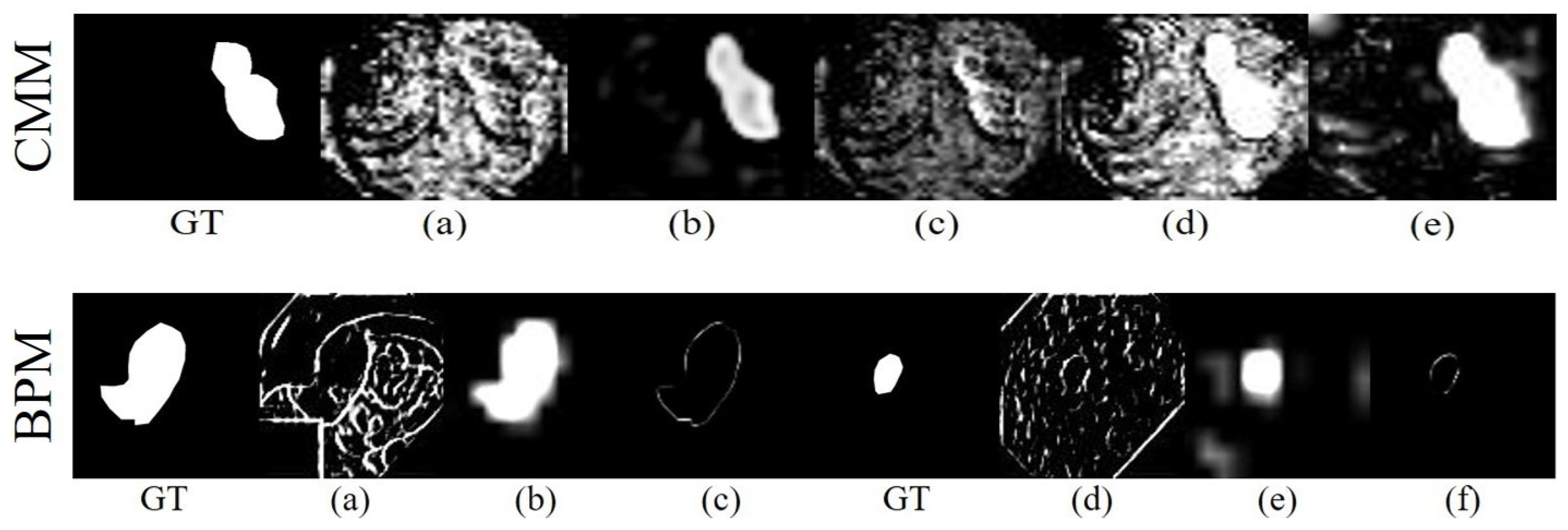
4.3. CMM and BPM Visualization

We visualized feature maps obtained from the CMM and BPM operations to explain complementary propagation.

4.3.1. Complementary Masking Visualization

To verify the effectiveness of the complementary multi-level aggregation, we sampled random channels from the low- and high-level representations and compared them after applying complementary information. In Figure 3-CMM, (a) and (b) denote relatively low-level and high-level features, respectively, whereas (c) is the complementary information masked by the high-level representation. We observed that the polyp regions were enhanced, and the discrepancy was diminished between (a)–(b) and (d)–(e) when applying the complementary information. The CMM in the first decoder propagated the refined representations to the next CMM and the second decoder. Following the complementary propagation, the second decoder could present the polyp regions under the discrepancy reduced representations.

4.3.2. Explicit Boundary Visualization

We have addressed the BPM generating explicit boundary information, and we visualized the lowest- and highest-level representations to observe the boundary. In Figure 3-BPM, (a), (d) and (b), (e) are the lowest- and highest-levels (i.e., $E_1$ and $D_4$), respectively. Each feature was randomly sampled from the channel-wise representations. Based on the properties of both levels, because the highest-level presented abstracted region information, it could be employed as a mask, which eliminated the background noise in the lowest-level representation. As a result, we obtained the explicit boundary features, as indicated in (c) and (f), following which the boundaries were propagated to the CMMs in the second decoder to clarify the polyp borderlines. By leveraging the explicit boundary and computing the boundary loss, COMMA could discriminate ambiguous polyp contexts more precisely.

4.4. Analysis of Loss Functions

4.4.1. Comparison of Loss Functions

To investigate the effectiveness of each loss function in the proposed hybrid loss function, a comparative experiment was performed between the hybrid loss function and other single loss functions in

Table 9. Comparison of the hybrid loss function and single loss functions.

Loss Function	Kvasir					ColonDB
	mDice	mIoU	${\mathit{S}}_{\mathit{m}}$	${\mathit{E}}_{\mathit{m}}$	MAE	mDice	mIoU	${\mathit{S}}_{\mathit{m}}$	${\mathit{E}}_{\mathit{m}}$	MAE
BCE	0.868	0.805	0.913	0.948	0.036	0.703	0.632	0.841	0.862	0.042
IoU	0.886	0.838	0.902	0.937	0.038	0.729	0.664	0.829	0.848	0.045
L1	0.886	0.835	0.903	0.941	0.032	0.751	0.681	0.843	0.869	0.038
wBCE	0.876	0.815	0.915	0.945	0.033	0.731	0.658	0.852	0.878	0.042
wIoU	0.892	0.842	0.905	0.940	0.037	0.762	0.699	0.845	0.870	0.041
Hybrid (wBCE + wIoU + L1)	0.901	0.852	0.919	0.951	0.027	0.754	0.689	0.849	0.897	0.037

. First, we compared the BCE, IoU, and L1 loss functions and observed that IoU loss performed better than BCE loss on mean dice and mean IoU, whereas BCE loss performed better than IoU loss on $S_m$ and $E_m$; however, L1 loss outperformed in most evaluation metrics. Second, to verify the effectiveness of the weighted loss function, BCE and weighted BCE were comapred along with IoU and weighted IoU. The weighted loss functions significantly improved the overall performance. This suggests that the weighted loss function allows the network to focus on the boundary information, leading to improved performance. Third, we compared the weighted BCE and the weighted IoU loss functions and found similar trends to the comparison of the BCE and IoU loss functions. Based on the results of this experiment, we concluded that the weighted IoU affected mDice and mIOU more than weighted BCE and L1, whereas weighted BCE affected $S_m$ and $E_m$ more. In addition, L1 loss, which exhibited the best MAE, helped the model to make pixel-by-pixel predictions with high confidence. Although some single loss functions outperformed the hybrid loss function on certain metrics, the proposed hybrid loss function significantly outperformed the alternatives on most evaluation metrics.

4.4.2. Weighted Loss Combination

We examine the combinations of the proposed hybrid loss function to observe the influence on local-global structure awareness and robustness against noisy annotations. As shown in

Table 10. Comparison of hybrid loss function combinations. $\alpha$, $\beta$, and $\gamma$ refer to the weights of ${\mathcal{L}}_{BCE}^w$, ${\mathcal{L}}_{IoU}^w$, and ${\mathcal{L}}_{L1}$, respectively.

$\mathit{\alpha }$ / $\mathit{\beta }$ / $\mathit{\gamma }$	Ver.	CVC-ClinicDB					ETIS
		mDice	mIoU	${\mathit{S}}_{\mathit{m}}$	${\mathit{E}}_{\mathit{m}}$	MAE	mDice	mIoU	${\mathit{S}}_{\mathit{m}}$	${\mathit{E}}_{\mathit{m}}$	MAE
1.0 / 1.0 / 0.0	(1)	0.929	0.886	0.956	0.984	0.008	0.700	0.639	0.839	0.880	0.020
1.0 / 0.5 / 0.5	(2)	0.933	0.892	0.945	0.981	0.008	0.712	0.649	0.833	0.863	0.018
0.5 / 1.0 / 0.5	(3)	0.926	0.884	0.959	0.986	0.009	0.689	0.630	0.844	0.886	0.021
0.5 / 0.5 / 1.0	(4)	0.925	0.883	0.947	0.980	0.007	0.682	0.624	0.835	0.860	0.017
1.0 / 1.0 / 1.0	(5)	0.933	0.891	0.956	0.985	0.007	0.711	0.648	0.844	0.887	0.015

, we excluded the L1 loss (ver. 1), the overall performance decreases. In ver. 2, which imposed more weights on the weighted BCE, mDice and mIoU increased because the wBCE enabled the network to learn the local structure, but $S_m$ and MAE were unsatisfactory. In contrast, higher weights for the wIoU (ver. 3) showed better local-global structure awareness ($S_m$) compared to other combinations, but this combination was unable to handle noisy labels for stable convergence. Although some combinations outperformed the equally weighted combinations in certain metrics (ver. 5), we adopted an equally weighted combination because it showed a satisfactory generalization performance.

5. Conclusions

This study has focused on the propagation of complementary multi-level aggregation to overcome multi-level distribution discrepancy. The proposed method, COMMA, leverages refined low- and high-level representations in a multi-decoder structure to discriminate polyps in ambiguous contexts. The decoder, which comprises a complementary masking module (CMM) and boundary propagation module (BPM), refines the complementary features by masking the low-level representation through the high-level representation, and propagates the complementary information to the next decoder. We also introduce a hybrid loss function combining weighted BCE, weighted IoU, and L1 distance loss to address class imbalance and noisy label problems. To verify the effectiveness of the proposed approach, we evaluated COMMA compared to existing segmentation methods on five benchmark datasets. COMMA achieved state-of-the-art performance, as well as significant generalization performance. In future work, we intend to study complementary multi-level aggregation to achieve greater memory efficiency and improve segmentation performance.

References

1. Granados-Romero, J.J.; Valderrama-Treviño, A.I.; Contreras-Flores, E.H.; Barrera-Mera, B.; Herrera Enríquez, M.; Uriarte-Ruíz, K.; Ceballos-Villalba, J.; Estrada-Mata, A.G.; Alvarado Rodríguez, C.; Arauz-Peña, G. Colorectal cancer: A review. Int. J. Res. Med. Sci. 2017, 5, 4667–4676. [Google Scholar] [CrossRef] [Green Version]
2. Schreuders, E.H.; Ruco, A.; Rabeneck, L.; Schoen, R.E.; Sung, J.J.; Young, G.P.; Kuipers, E.J. Colorectal cancer screening: A global overview of existing programmes. Gut 2015, 64, 1637–1649. [Google Scholar] [CrossRef]
3. Mármol, I.; Sánchez-de Diego, C.; Pradilla Dieste, A.; Cerrada, E.; Rodriguez Yoldi, M.J. Colorectal carcinoma: A general overview and future perspectives in colorectal cancer. Int. J. Mol. Sci. 2017, 18, 197. [Google Scholar] [CrossRef] [Green Version]
4. Siegel, R.L.; Miller, K.D.; Goding Sauer, A.; Fedewa, S.A.; Butterly, L.F.; Anderson, J.C.; Cercek, A.; Smith, R.A.; Jemal, A. Colorectal cancer statistics, 2020. CA Cancer J. Clin. 2020, 70, 145–164. [Google Scholar] [CrossRef] [PubMed] [Green Version]
5. Mamonov, A.V.; Figueiredo, I.N.; Figueiredo, P.N.; Tsai, Y.H.R. Automated polyp detection in colon capsule endoscopy. IEEE Trans. Med. Imaging 2014, 33, 1488–1502. [Google Scholar] [CrossRef] [Green Version]
6. Tajbakhsh, N.; Gurudu, S.R.; Liang, J. Automated polyp detection in colonoscopy videos using shape and context information. IEEE Trans. Med. Imaging 2015, 35, 630–644. [Google Scholar] [CrossRef] [PubMed]
7. Yu, L.; Chen, H.; Dou, Q.; Qin, J.; Heng, P.A. Integrating online and offline three-dimensional deep learning for automated polyp detection in colonoscopy videos. IEEE J. Biomed. Health Inform. 2016, 21, 65–75. [Google Scholar] [CrossRef] [PubMed]
8. Long, J.; Shelhamer, E.; Darrell, T. Fully convolutional networks for semantic segmentation. In Proceedings of the IEEE Conference on Computer Vision and Pattern Recognition, Boston, MA, USA, 7–12 June 2015; pp. 3431–3440. [Google Scholar]
9. Ronneberger, O.; Fischer, P.; Brox, T. U-net: Convolutional networks for biomedical image segmentation. In Proceedings of the International Conference on Medical Image Computing and Computer-Assisted Intervention, Munich, Germany, 5–9 October 2015; Springer: Berlin/Heidelberg, Germany, 2015; pp. 234–241. [Google Scholar]
10. He, K.; Gkioxari, G.; Dollár, P.; Girshick, R. Mask r-cnn. In Proceedings of the IEEE International Conference on Computer Vision, Venice, Italy, 22–29 October 2017; pp. 2961–2969. [Google Scholar]
11. Brandao, P.; Mazomenos, E.; Ciuti, G.; Caliò, R.; Bianchi, F.; Menciassi, A.; Dario, P.; Koulaouzidis, A.; Arezzo, A.; Stoyanov, D. Fully convolutional neural networks for polyp segmentation in colonoscopy. In Medical Imaging 2017: Computer-Aided Diagnosis; SPIE: Orlando, FL, USA, 2017; Volume 10134, pp. 101–107. [Google Scholar]
12. Ji, G.P.; Chou, Y.C.; Fan, D.P.; Chen, G.; Fu, H.; Jha, D.; Shao, L. Progressively normalized self-attention network for video polyp segmentation. In Proceedings of the International Conference on Medical Image Computing and Computer-Assisted Intervention, Strasbourg, France, 27 September–1 October 2021; Springer: Berlin/Heidelberg, Germany, 2021; pp. 142–152. [Google Scholar]
13. Wei, J.; Hu, Y.; Zhang, R.; Li, Z.; Zhou, S.K.; Cui, S. Shallow attention network for polyp segmentation. In Proceedings of the International Conference on Medical Image Computing and Computer-Assisted Intervention, Strasbourg, France, 27 September–1 October 2021; Springer: Berlin/Heidelberg, Germany, 2021; pp. 699–708. [Google Scholar]
14. Wang, T.; Zhang, L.; Wang, S.; Lu, H.; Yang, G.; Ruan, X.; Borji, A. Detect globally, refine locally: A novel approach to saliency detection. In Proceedings of the IEEE Conference on Computer Vision and Pattern Recognition, Salt Lake City, UT, USA, 18–23 June 2018; pp. 3127–3135. [Google Scholar]
15. Wu, Z.; Su, L.; Huang, Q. Cascaded partial decoder for fast and accurate salient object detection. In Proceedings of the IEEE Conference on Computer Vision and Pattern Recognition, Long Beach, CA, USA, 12–20 June 2019; pp. 3907–3916. [Google Scholar]
16. Zhang, P.; Wang, D.; Lu, H.; Wang, H.; Ruan, X. Amulet: Aggregating multi-level convolutional features for salient object detection. In Proceedings of the IEEE International Conference on Computer Vision, Venice, Italy, 22–29 October 2017; pp. 202–211. [Google Scholar]
17. Zhou, Z.; Siddiquee, M.M.R.; Tajbakhsh, N.; Liang, J. Unet++: A nested u-net architecture for medical image segmentation. In Deep Learning in Medical Image Analysis and Multimodal Learning for Clinical Decision Support; Springer: Berlin/Heidelberg, Germany, 2018; pp. 3–11. [Google Scholar]
18. Jha, D.; Smedsrud, P.H.; Johansen, D.; de Lange, T.; Johansen, H.D.; Halvorsen, P.; Riegler, M.A. A comprehensive study on colorectal polyp segmentation with ResUNet++, conditional random field and test-time augmentation. IEEE J. Biomed. Health Inform. 2021, 25, 2029–2040. [Google Scholar] [CrossRef]
19. Jha, D.; Smedsrud, P.H.; Riegler, M.A.; Johansen, D.; De Lange, T.; Halvorsen, P.; Johansen, H.D. Resunet++: An advanced architecture for medical image segmentation. In Proceedings of the 2019 IEEE International Symposium on Multimedia (ISM), San Diego, CA, USA, 9–11 December 2019; pp. 225–2255. [Google Scholar]
20. Fang, Y.; Chen, C.; Yuan, Y.; Tong, K.y. Selective feature aggregation network with area-boundary constraints for polyp segmentation. In Proceedings of the International Conference on Medical Image Computing and Computer-Assisted Intervention, Shenzhen, China, 13–17 October 2019; Springer: Berlin/Heidelberg, Germany, 2019; pp. 302–310. [Google Scholar]
21. Zhang, R.; Li, G.; Li, Z.; Cui, S.; Qian, D.; Yu, Y. Adaptive context selection for polyp segmentation. In Proceedings of the International Conference on Medical Image Computing and Computer-Assisted Intervention, Lima, Peru, 4–8 October 2020; Springer: Berlin/Heidelberg, Germany, 2020; pp. 253–262. [Google Scholar]
22. Patel, K.; Bur, A.M.; Wang, G. Enhanced u-net: A feature enhancement network for polyp segmentation. In Proceedings of the 2021 18th Conference on Robots and Vision (CRV), Burnaby, BC, Canada, 26–28 May 2021; pp. 181–188. [Google Scholar]
23. Murugesan, B.; Sarveswaran, K.; Shankaranarayana, S.M.; Ram, K.; Joseph, J.; Sivaprakasam, M. Psi-Net: Shape and boundary aware joint multi-task deep network for medical image segmentation. In Proceedings of the 2019 41st Annual International Conference of the IEEE Engineering in Medicine and Biology Society (EMBC), Berlin, Germany, 23–27 July 2019; pp. 7223–7226. [Google Scholar]
24. Lee, C.Y.; Xie, S.; Gallagher, P.; Zhang, Z.; Tu, Z. Deeply-supervised nets. In Proceedings of the Artificial Intelligence and Statistics, San Diego, CA, USA, 9–12 May 2015; pp. 562–570. [Google Scholar]
25. Wang, D.; Hao, M.; Xia, R.; Zhu, J.; Li, S.; He, X. MSB-Net: Multi-Scale Boundary Net for Polyp Segmentation. In Proceedings of the 2021 IEEE 10th Data Driven Control and Learning Systems Conference (DDCLS), Suzhou, China, 14–16 May 2021; pp. 88–93. [Google Scholar]
26. Cao, F.; Gao, C.; Ye, H. A novel method for image segmentation: Two-stage decoding network with boundary attention. Int. J. Mach. Learn. Cybern. 2021, 1–13. [Google Scholar] [CrossRef]
27. Fan, D.P.; Ji, G.P.; Zhou, T.; Chen, G.; Fu, H.; Shen, J.; Shao, L. Pranet: Parallel reverse attention network for polyp segmentation. In Proceedings of the International Conference on Medical Image Computing and Computer-Assisted Intervention, Lima, Peru, 4–8 October 2020; Springer: Berlin/Heidelberg, Germany, 2020; pp. 263–273. [Google Scholar]
28. Chen, S.; Tan, X.; Wang, B.; Hu, X. Reverse attention for salient object detection. In Proceedings of the European Conference on Computer Vision (ECCV), Munich, Germany, 8–14 September 2018; pp. 234–250. [Google Scholar]
29. Wei, J.; Wang, S.; Huang, Q. F3Net: Fusion, Feedback and Focus for Salient Object Detection. In Proceedings of the AAAI Conference on Artificial Intelligence, Hilton, NY, USA, 7–12 February 2020; Volume 34, pp. 12321–12328. [Google Scholar]
30. Ghosh, A.; Kumar, H.; Sastry, P. Robust loss functions under label noise for deep neural networks. In Proceedings of the AAAI Conference on Artificial Intelligence, San Francisco, CA, USA, 4–9 February 2017; Volume 31. [Google Scholar]
31. Wang, G.; Liu, X.; Li, C.; Xu, Z.; Ruan, J.; Zhu, H.; Meng, T.; Li, K.; Huang, N.; Zhang, S. A noise-robust framework for automatic segmentation of COVID-19 pneumonia lesions from CT images. IEEE Trans. Med. Imaging 2020, 39, 2653–2663. [Google Scholar] [CrossRef]
32. He, K.; Zhang, X.; Ren, S.; Sun, J. Deep residual learning for image recognition. In Proceedings of the IEEE Conference on Computer Vision and Pattern Recognition, Las Vegas, NV, USA, 27–30 June 2016; pp. 770–778. [Google Scholar]
33. Gao, S.; Cheng, M.M.; Zhao, K.; Zhang, X.Y.; Yang, M.H.; Torr, P.H. Res2net: A new multi-scale backbone architecture. IEEE Trans. Pattern Anal. Mach. Intell. 2019, 43, 652–662. [Google Scholar] [CrossRef] [PubMed] [Green Version]
34. He, K.; Zhang, X.; Ren, S.; Sun, J. Identity mappings in deep residual networks. In Proceedings of the European Conference on Computer Vision, Amsterdam, The Netherlands, 8–16 October 2016; Springer: Berlin/Heidelberg, Germany, 2016; pp. 630–645. [Google Scholar]
35. Jain, V.; Seung, S. Natural image denoising with convolutional networks. Adv. Neural Inf. Process. Syst. 2008, 21, 769–776. [Google Scholar]
36. Dong, C.; Loy, C.C.; He, K.; Tang, X. Image super-resolution using deep convolutional networks. IEEE Trans. Pattern Anal. Mach. Intell. 2015, 38, 295–307. [Google Scholar] [CrossRef] [Green Version]
37. Zhao, J.X.; Liu, J.J.; Fan, D.P.; Cao, Y.; Yang, J.; Cheng, M.M. EGNet: Edge guidance network for salient object detection. In Proceedings of the IEEE International Conference on Computer Vision, Seoul, Korea, 27–28 October 2019; pp. 8779–8788. [Google Scholar]
38. Jha, D.; Smedsrud, P.H.; Riegler, M.A.; Halvorsen, P.; Lange, T.d.; Johansen, D.; Johansen, H.D. Kvasir-seg: A segmented polyp dataset. In Proceedings of the International Conference on Multimedia Modeling, Daejeon, Korea, 5–8 January 2020; Springer: Berlin/Heidelberg, Germany, 2020; pp. 451–462. [Google Scholar]
39. Bernal, J.; Sánchez, F.J.; Fernández-Esparrach, G.; Gil, D.; Rodríguez, C.; Vilariño, F. WM-DOVA maps for accurate polyp highlighting in colonoscopy: Validation vs. saliency maps from physicians. Comput. Med. Imaging Graph. 2015, 43, 99–111. [Google Scholar] [CrossRef]
40. Bernal, J.; Sánchez, J.; Vilarino, F. Towards automatic polyp detection with a polyp appearance model. Pattern Recognit. 2012, 45, 3166–3182. [Google Scholar] [CrossRef]
41. Silva, J.; Histace, A.; Romain, O.; Dray, X.; Granado, B. Toward embedded detection of polyps in wce images for early diagnosis of colorectal cancer. Int. J. Comput. Assist. Radiol. Surg. 2014, 9, 283–293. [Google Scholar] [CrossRef] [PubMed]
42. Vázquez, D.; Bernal, J.; Sánchez, F.J.; Fernández-Esparrach, G.; López, A.M.; Romero, A.; Drozdzal, M.; Courville, A. A benchmark for endoluminal scene segmentation of colonoscopy images. J. Healthc. Eng. 2017, 2017, 4037190. [Google Scholar] [CrossRef] [PubMed]
43. Chen, Z.; Xu, Q.; Cong, R.; Huang, Q. Global context-aware progressive aggregation network for salient object detection. In Proceedings of the AAAI Conference on Artificial Intelligence, Hilton, NY, USA, 7–12 February 2020; Volume 34, pp. 10599–10606. [Google Scholar]
44. Fan, D.P.; Cheng, M.M.; Liu, Y.; Li, T.; Borji, A. Structure-measure: A new way to evaluate foreground maps. In Proceedings of the IEEE International Conference on Computer Vision, Venice, Italy, 22–29 October 2017; pp. 4548–4557. [Google Scholar]
45. Fan, D.P.; Gong, C.; Cao, Y.; Ren, B.; Cheng, M.M.; Borji, A. Enhanced-alignment measure for binary foreground map evaluation. arXiv 2018, arXiv:1805.10421. [Google Scholar]
46. Zhang, Z.; Liu, Q.; Wang, Y. Road extraction by deep residual u-net. IEEE Geosci. Remote Sens. Lett. 2018, 15, 749–753. [Google Scholar] [CrossRef] [Green Version]
Figure 1. Overall architecture of proposed COMMA.
Applsci 12 02114 g001
Figure 2. Qualitative comparison with existing methods.
Applsci 12 02114 g002
Figure 3. Visualization of complementary masking and explicit boundary generation.
Applsci 12 02114 g003