
Bioremediation of Hydrocarbon-Polluted Soil: Evaluation of Different Operative Parameters

 ,
,  ,
,  and
and 
Abstract
:1. Introduction
2. Materials and Methods
2.1. Study Cases Overview
- Microcosms test (test M), based on a small amount of polluted soil (200 g)
- Bench test (test B), based on a larger polluted mass (around 38 kg).
2.1.1. Microcosms Test
2.1.2. Bench Test
2.2. Studied Factors
2.2.1. Factors and Levels for the Test M
2.2.2. Factors and Levels for the Test B
2.3. Experimental Setup
2.3.1. Test M
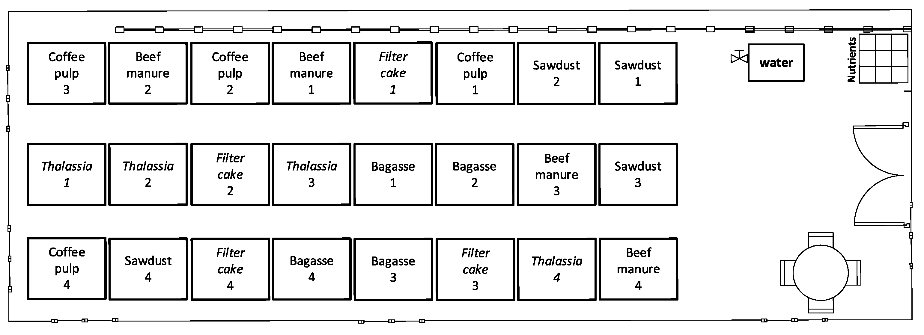
2.3.2. Test B
2.4. Response Variable
2.4.1. Determination of the TPH Concentration in the Test M
2.4.2. Determination of the TPH Concentration in Test B
2.5. Hydrocarbon Removal
2.5.1. Statistical Analysis
2.5.2. Kinetics Analysis
3. Results
3.1. Statistical Analysis
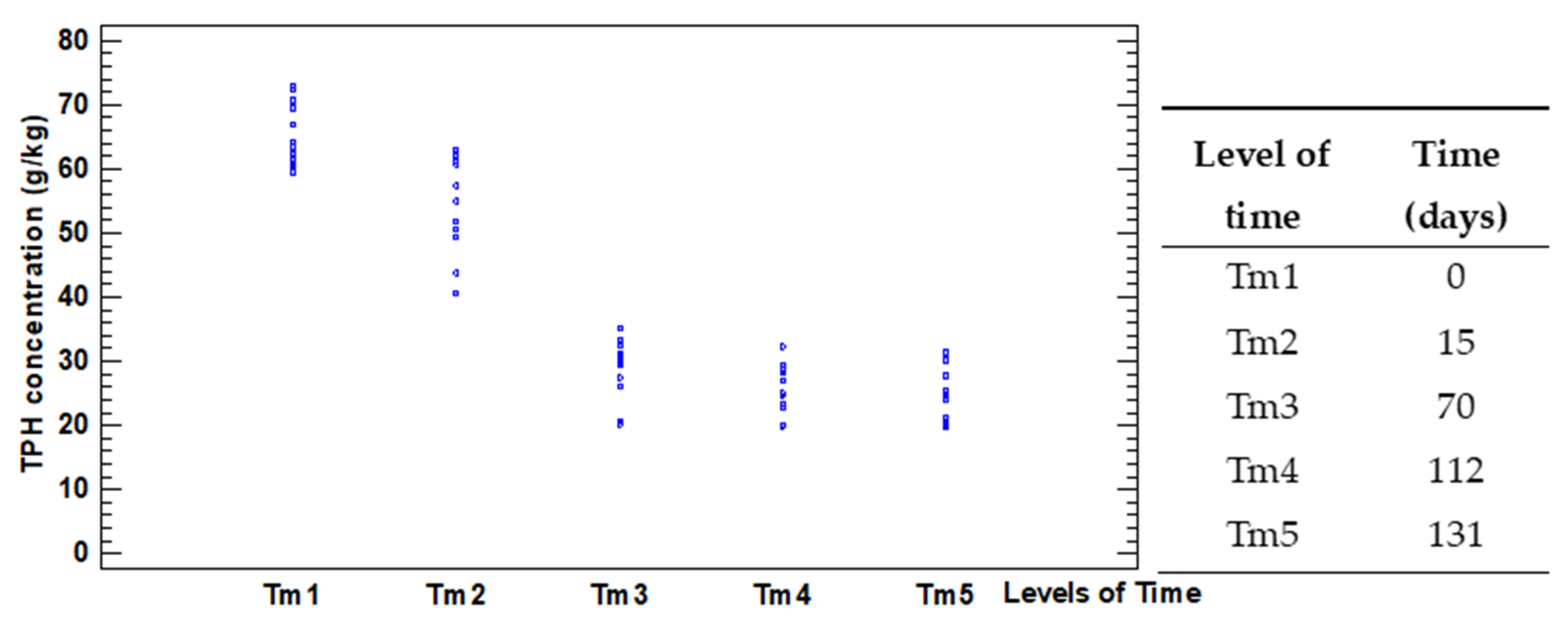
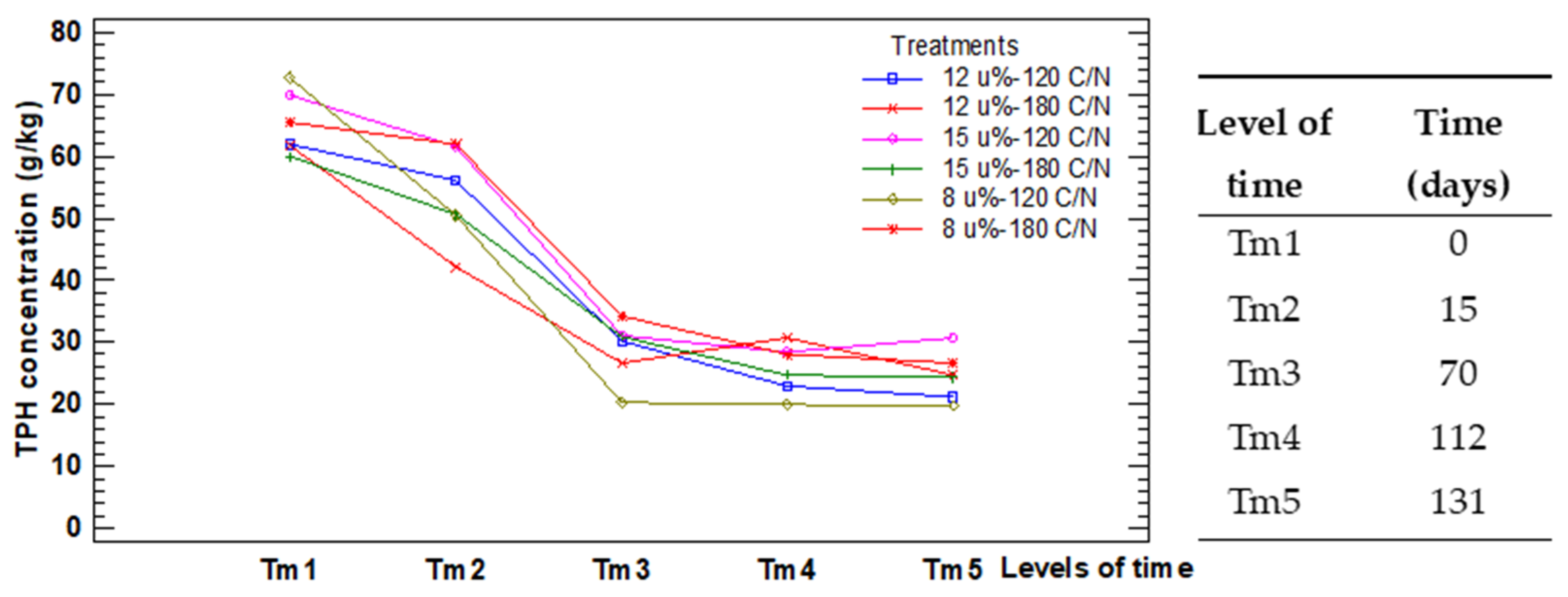
3.1.1. Test M
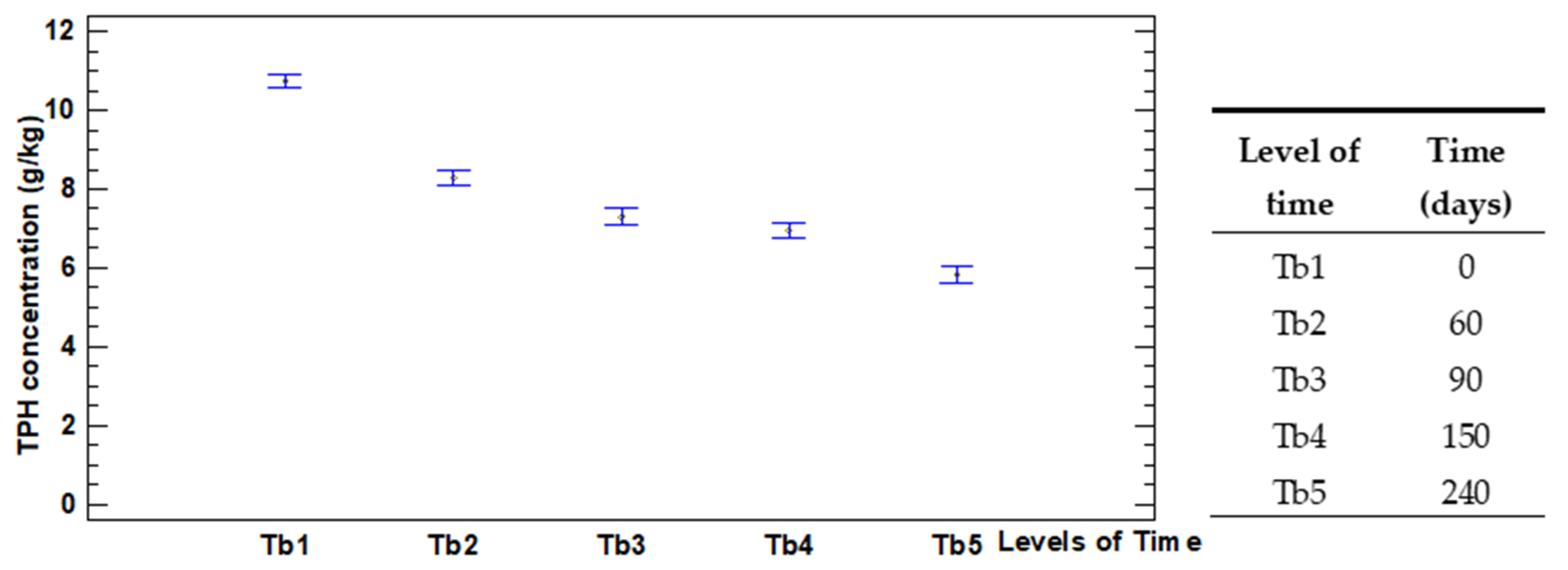
3.1.2. Test B
3.2. Kinetics Analysis Results
3.2.1. Kinetic Analysis of Test M
3.2.2. Kinetic Analysis of Test B
4. Discussion
5. Conclusions
Author Contributions
Funding
Institutional Review Board Statement
Informed Consent Statement
Data Availability Statement
Acknowledgments
Conflicts of Interest
Appendix A


Appendix B
References
- Koolivand, A.; Abtahi, H.; Parhamfar, M.; Didehdar, M.; Saeedi, R.; Fahimirad, S. Biodegradation of high concentrations of petroleum compounds by using indigenous bacteria isolated from petroleum hydrocarbons-rich sludge: Effective scale-up from liquid medium to composting process. J. Environ. Manag. 2019, 248, 109228. [Google Scholar] [CrossRef] [PubMed]
- Shahryar, J. Chapter 3: Environmental Impacts of the Petroleum Industry. In Petroleum Waste Treatment and Pollution Control; Shahryar, J., Ed.; Butterworth-Heinemann: Oxford, UK; Elsevier Inc.: Amsterdam, The Netherlands, 2017; Volume 3, pp. 86–115. ISBN 978-0-12-809243-9. [Google Scholar] [CrossRef]
- Bosco, F.; Casale, A.; Mazzarino, I.; Godio, A.; Ruffino, B.; Mollea, C.; Chiampo, F. Microcosm evaluation of bioaugmentation and biostimulation efficacy on diesel-contaminated soil. J. Chem. Technol. Biotechnol. 2019, 94, 904–912. [Google Scholar] [CrossRef]
- Hu, G.; Li, J.; Zeng, G. Recent development in the treatment of oily sludge from petroleum industry: A review. J. Hazard. Mater. 2013, 261, 470–490. [Google Scholar] [CrossRef] [PubMed]
- Li, J.; Guo, C.; Lu, G.; Yi, X.; Dang, Z. Bioremediation of Petroleum-Contaminated Acid Soil by a Constructed Bacterial Consortium Immobilized on Sawdust: Influences of Multiple Factors. Water Air Soil Pollut. 2016, 227, 444. [Google Scholar] [CrossRef]
- Kaczorek, E.; Smułek, W. Effective scale-up from liquid medium to composting process. Processes 2021, 9, 1130. [Google Scholar] [CrossRef]
- Johnston, J.; Cushing, L. Chemical Exposures, Health, and Environmental Justice in Communities Living on the Fenceline of Industry. Curr. Environ. Health Rep. 2020, 7, 48–57. [Google Scholar] [CrossRef]
- Castro, D.J.; Gutiérrez, O.; Poma, J.R.; Bermúdez, J.; Demichela, M. Environmental monitoring in a Cuban oil storage plant to characterize the hydrocarbons pollution exposure in the fence-line community. In Oil and Gas Industry, Proceedings of the 31st European and Safety Reliability (ESREL 2021), Angers, France, 19–23 September 2021; Castanier, B., Cepin, M., Bigaud, D., Berenguer, C., Eds.; Research Publishing Services: Singapore, 2021; pp. 2299–2304. ISBN 978-981-18-2016-8. [Google Scholar] [CrossRef]
- Gospodarek, J.; Petryszak, P.; Kołoczek, H. The effect of the bioremediation of soil contaminated with petroleum derivatives on the occurrence of epigeic and edaphic fauna. Bioremediat. J. 2016, 20, 38–53. [Google Scholar] [CrossRef]
- Margesin, R.; Zimmerbauer, A.; Schinner, F. Monitoring of bioremediation by soil biological activities. Chemosphere 2000, 40, 339–346. [Google Scholar] [CrossRef]
- Raffa, C.M.; Chiampo, F.; Godio, A.; Vergnano, A.; Bosco, F.; Ruffino, B. Kinetics and Optimization by Response Surface Methodology of Aerobic Bioremediation. Geoelectrical Parameter Monitoring. Appl. Sci. 2020, 10, 405. [Google Scholar] [CrossRef] [Green Version]
- Basak, G.; Hazra, C.; Sen, R. Biofunctionalized nanomaterials for in situ clean-up of hydrocarbon contamination: A quantum jump in global bioremediation research. J. Environ. Manag. 2020, 256, 109913. [Google Scholar] [CrossRef]
- Poddar, K.; Sarkar, D.; Sarkar, A. Construction of potential bacterial consortia for efficient hydrocarbon degradation. Int. Biodeterior. Biodegrad. 2019, 144, 104770. [Google Scholar] [CrossRef]
- Poi, G.; Shahsavari, D.; Aburto-Medina, A.; Mok, P.C.; Ball, A.S. Large scale treatment of total petroleum-hydrocarbon contaminated groundwater using bioaugmentation. J. Environ. Manag. 2018, 214, 157–163. [Google Scholar] [CrossRef]
- Varjani, S.J.; Gnansounou, E.; Pandey, A. Comprehensive review on toxicity of persistent organic pollutants from petroleum refinery waste and their degradation by microorganisms. Chemosphere 2019, 188, 280–291. [Google Scholar] [CrossRef] [PubMed]
- Adetutu, E.M.; Bird, C.; Kadali, K.K.; Bueti, A.; Shahsavari, E.; Taha, M.; Patil, S.; Sheppard, P.J.; Makadia, T.; Simons, K.L.; et al. Exploiting the intrinsic hydrocarbon-degrading microbial capacities in oil tank bottom sludge and waste soil for sludge bioremediation. Int. J. Environ. Sci. Technol. 2015, 12, 1427–1436. [Google Scholar] [CrossRef]
- USEPA. Cleaning up the Nation’s Waste Sites: Markets and Technology Trends; EPA 542-R-04-015; US Environmental Protection Agency: Washington, DC, USA, 2004.
- Lim, M.W.; Lau, E.V.; Poh, P.E. A comprehensive guide of remediation technologies for oil contaminated soil-Present works and future directions. Mar. Pollut. Bull. 2016, 109, 14–45. [Google Scholar] [CrossRef] [PubMed]
- Ossai, I.C.; Ahmed, A.; Hassan, A.; Shahul, F.; Ball, A.S. Remediation of soil and water contaminated with petroleum hydrocarbon: A review. Environ. Technol. Innov. 2020, 17, 100526. [Google Scholar] [CrossRef]
- Tran, H.-T.; Lin, C.; Bui, X.-T.; Ngo, H.-H.; Cheruiyot, N.K.; Hoang, H.-G.; Vu, C.-T. Aerobic composting remediation of petroleum hydrocarbon-contaminated soil. Current and future perspectives. Sci. Total Environ. 2021, 753, 142250. [Google Scholar] [CrossRef]
- Calvo, C.; Rodríguez-Calvo, A.; Robledo-Mahón, T.; Manzanera, M.; González-López, J.; Aranda, E.; Silva-Castro, G.A. Biostimulation of crude oil-polluted soils: Influence of initial physicochemical and biological characteristics of soil. J. Environ. Sci. Technol. 2019, 16, 4925–4934. [Google Scholar] [CrossRef]
- Yanto, D.H.Y.; Hidayat, A.; Tachibana, S. Periodical biostimulation with nutrient addition and bioaugmentation using mixed fungal cultures to maintain enzymatic oxidation during extended bioremediation of oily soil microcosms. Int. Biodeterior. Biodegrad. 2017, 116, 112–123. [Google Scholar] [CrossRef]
- Wu, M.; Dick, W.A.; Li, W.; Wang, X.; Yang, Q.; Wang, T.; Xu, L.; Zhang, M.; Chen, L. Bioaugmentation and biostimulation of hydrocarbon degradation and the microbial community in a petroleum-contaminated soil. Int. Biodeterior. Biodegrad. 2016, 107, 158–164. [Google Scholar] [CrossRef]
- Juwarkar, A.A.; Singh, S.K.; Mudhoo, A.A. A comprehensive overview of elements in bioremediation. Rev. Env. Sci. Biotechnol. 2010, 9, 215–288. [Google Scholar] [CrossRef]
- Haghollahi, A.; Hassan, A.F.; Schaffie, M. The effect of soil type on the bioremediation of petroleum contaminated soils. J. Environ. Manag. 2016, 180, 197–201. [Google Scholar] [CrossRef] [PubMed]
- Bidja Abena, M.T.; Li, T.; Shah, M.N.; Zhong, W. Biodegradation of total petroleum hydrocarbons (TPH) in highly contaminated soils by natural attenuation and bioaugmentation. Chemosphere 2019, 234, 864–874. [Google Scholar] [CrossRef] [PubMed]
- Casale, A.; Bosco, F.; Chiampo, F.; Franco, D.; Ruffino, B.; Godio, A.; Pujari, P.R. Soil microcosm set up for a bioremediation study. In Proceedings of the Sixth International Conference on Advances in Bio-Informatics, Bio-Technology and Environmental Engineering—ABBE 2018, Zurich, Switzerland, 28–29 April 2018; The IRED: New York, NY, USA, 2018; pp. 12–15. [Google Scholar] [CrossRef]
- Simpanen, S.; Dahl, M.; Gerlach, M.; Mikkonen, A.; Malk, V.; Mikola, J.; Romantschuk, M. Biostimulation proved to be the most efficient method in the comparison of in situ soil remediation treatments after a simulated oil spill accident. Environ. Sci. Pollut. Res. 2016, 23, 25024–25038. [Google Scholar] [CrossRef] [Green Version]
- Rene, E.R.; Jo, M.S.; Kim, S.H.; Park, H.S. Statistical analysis of main and interaction effects during the removal of BTEX mixtures in batch conditions, using wastewater treatment plant sludge microbes. Int. J. Environ. Sci. Technol. 2007, 4, 177–182. [Google Scholar] [CrossRef] [Green Version]
- Box, G.E.; Hunter, W.G.; Hunter, J.S. Statistics for Experimenters, 2nd ed.; John Wiley & Sons, Inc.: New York, NY, USA, 1978; pp. 1–640. [Google Scholar]
- Montgomery, D.C. Design and Analysis of Experiments, 9th ed.; John Wiley & Sons, Inc.: Scottsdale, AZ, USA, 2020; pp. 1–752. ISBN 978-1-119-32093-7. [Google Scholar]
- Gutiérrez, H.; de la Vara, R. Analysis and Design of Experiments, 3rd ed.; MCGRAW-HILL INTERAMERICANA, S.A., Ed.; McGraw-Hill: México City, Mexico, 2012; pp. 1–506. ISBN 978-607-15-0725-9. (In Spanish) [Google Scholar]
- Gutiérrez, O.; Castro, D.; Viera, O.; Casals, E.; Rabassa, D. Kinetic of hydrocarbon degradation by biopile at a bench-scale. Tecnol. Química 2021, 41, 349–369. [Google Scholar]
- Komilis, D.P.; Vrohidou, A.E.K.; Voudrias, E.A. Kinetics of Aerobic Bioremediation of a Diesel-Contaminated Sandy Soil: Effect of Nitrogen Addition. Water Air Soil Pollut. 2010, 208, 193–208. [Google Scholar] [CrossRef]
- Tellechea, F.R.F.; Martins, M.A.; da Silva, A.A.; Forestieri de Gama-Rodrigues, E.; Martins, M.L.M. Use of sugarcane filter cake and nitrogen, phosphorus and potassium fertilization in the process of bioremediation of soil contaminated with diesel. Env. Sci. Pollut. Res. 2016, 23, 18027–18033. [Google Scholar] [CrossRef]
- Gholami-Shiri, J.; Mowla, D.; Dehghani, S.; Setoodeh, V. Exploitation of novel synthetic bacterial consortia for biodegradation of oily-sludge TPH of Iran gas and oil refineries. J. Environ. Chem. Eng. 2021, 19, 1263–1276. [Google Scholar] [CrossRef]
- Oualha, M.; Al-Kaabi, N.; Al-Ghouti, M.; Zouari, N. Identification and overcome of limitations of weathered oil hydrocarbons bioremediation by an adapted Bacillus sorensis strain. J. Environ. Manag. 2019, 250, 109455. [Google Scholar] [CrossRef]
- Aziz, S.; Ali, M.I.; Farooq, U.; Jamal, A.; Liu, F.J.; He, H.; Guo, H.; Urynowicz, M.; Huang, Z. Enhanced bioremediation of diesel range hydrocarbons in soil using biochar made from organic wastes. Env. Monit. Assess. 2020, 192, 569. [Google Scholar] [CrossRef] [PubMed]
- Zhang, C.; Wu, D.; Ren, H. Bioremediation of oil contaminated soil using agricultural wastes via microbial consortium. Sci. Rep. 2020, 10, 9188. [Google Scholar] [CrossRef] [PubMed]
- Castro, D.; Gonález, Y.; Gutiérrez, O.; Viera, O.; Casals, E.; Rabassa, D.; Demichela, M. QFD to determine experimental biopiles requirements, evaluated at bench-scaleas a resilient strategy against soil contamination with oil residues. Chem. Eng. Trans. 2021; accepted. [Google Scholar]
- USEPA. Chapter IV: Biopiles. In How to Evaluate Alternative Cleanup Technologies for Underground Storage Tank Sites. A Guide for Corrective Action Plan Reviewers; EPA 510-B-17-003; United Stated Environmental Protection Agency (USEPA): Washington, DC, USA, 2017; pp. 1–27. [Google Scholar]
- Gutiérrez, O.; Castro, D.; Viera, O.; Casals, E.; Rabassa, D. Engineering design and assembly of experimental units for the bioremediation of petroleum waste on a bench-scale. Tecnol. Química 2020, 40, 546–562. [Google Scholar]
- Casals, E.; Rabassa, D.; Viera, O.; Gutiérrez, O.; Castro, D. Abiotic factors behavior in petrolized residues biorremediation by biopiles at semi-pilot scale. Cent. Azúcar 2020, 47, 36–46. [Google Scholar]
- NC 20:1999; Geotechnics: Determination of the Granulometry of Soils; Norma Cubana (Cuban Standard). Oficina Nacional de Normalización (ONN): Havana, Cuba, 1999. (In Spanish)
- NC 59:2000; Geotechnics. Geotechnical Classification of Soils; Norma Cubana (Cuban Standard). Oficina Nacional de Normalización (ONN): Havana, Cuba, 2000. (In Spanish)
- NC 819: 2017; Management of Waste from the Bottom of Oil Storage Tanks and Its Derivatives; Norma Cubana (Cuban Standard). Oficina Nacional de Normalización (ONN): Havana, Cuba, 2017. (In Spanish)
- Bosco, F.; Casale, A.; Chiampo, F.; Godio, A. Removal of diesel oil in soil microcosms and implication for geophysical monitoring. Water 2019, 11, 1661. [Google Scholar] [CrossRef] [Green Version]
- Lin, T.C.; Pan, P.T.; Cheng, S.S. Ex situ bioremediation of oil-contaminated soil. J. Hazard. Mater. 2010, 116, 27–34. [Google Scholar] [CrossRef]
- Gomez, F.; Sartaj, M. Optimization of field scale biopiles for bioremediation of petroleum hydrocarbon contaminated soil at low temperature conditions by response surface methodology (RSM). Int. Biodeterior. Biodegrad. 2014, 89, 103–109. [Google Scholar] [CrossRef]
- Khayati, G.; Barati, M. Bioremediation of Petroleum Hydrocarbon Contaminated Soil: Optimization Strategy Using Taguchi Design of Experimental (DOE) Methodology. Environ. Process. 2017, 4, 451–461. [Google Scholar] [CrossRef]
- Poorsoleiman, M.S.; Hosseini, S.A.; Etminan, A.; Abtahi, H.; Koolivand, A. Effect of two-step bioaugmentation of an indigenous bacterial strain isolated from oily waste sludge on petroleum hydrocarbons biodegradation: Scaling-up from a liquid mineral medium to a two-stage composting process. Environ. Technol. Innov. 2020, 17, 100558. [Google Scholar] [CrossRef]


| Operative Conditions | Microcosms (Test M) | Biopiles (Test B) |
|---|---|---|
| Response variable | TPH | TPH |
| Factor 1-Treatments (6 categorical levels) | M1 (8 WC%-120 C/N) | B1 (sugarcane bagasse) |
| M2 (8 WC%-180 C/N) | B2 (sugarcane filter cake) | |
| M3 (12 WC%-120 C/N) | B3 (sawdust) | |
| M4 (12 WC%-180 C/N) | B4 (coffee pulp) | |
| M5 (15 WC%-120 C/N) | B5 (beef manure) | |
| M6 (15 WC%-180 C/N) | B6 (Thalassia testudinum) | |
| Factor 2-Time (5 levels) | 0 | 0 |
| 15 days | 60 days | |
| 70 days | 90 days | |
| 112 days | 150 days | |
| 131 days | 240 days | |
| Mass | 200 g | 38 kg |
| Pollutant | Diesel oil | Oily Sludge |
| Water content (WC%) | 8% 12% 15% | 20% |
| Carbon to nitrogen ratio (C/N) | 60 120 180 300 | 10 |
| Kind of soil | Sandy soil | Sandy soil |
| pH | 6–8 | 6–8 |
| Source | Sum of Squares | Df | Mean Square | F-Ratio | p-Value |
|---|---|---|---|---|---|
| Main Effects | |||||
| Treatments | 537.43 | 5 | 107.47 | 72.21 | 0.000 |
| Time | 16,735.40 | 4 | 4183.84 | 2810.60 | 0.000 |
| Interactions | |||||
| Treatments·Time | 845.22 | 20 | 42.27 | 28.39 | 0.000 |
| Residual | 44.66 | 30 | 1.49 | ||
| Total (corrected) | 18162.70 | 59 | |||
| Treatments | Mean (g·kg−1) | Lower Limit (g·kg−1) | Upper Limit (g·kg−1) | Homogeneous Groups |
|---|---|---|---|---|
| u8%-C/N = 120 | 36.65 | 35.86 | 37.44 | X |
| u12%-C/N = 180 | 37.25 | 36.46 | 38.04 | X X |
| u15%-C/N = 180 | 38.15 | 37.36 | 38.94 | X X |
| u12%-C/N = 120 | 38.48 | 37.69 | 39.27 | X |
| u8%-C/N = 180 | 43.28 | 42.49 | 44.07 | X |
| u15%-C/N = 120 | 44.36 | 43.57 | 45.15 | X |
| Standard Deviation: 0.385823 | ||||
| Source | Sum of Squares | Df | Mean Square | F-Ratio | p-Value |
|---|---|---|---|---|---|
| Main Effects | |||||
| Treatments | 23.77 | 5 | 4.75 | 11.54 | 0.000 |
| Time | 315.93 | 4 | 78.98 | 191.81 | 0.000 |
| Interactions | |||||
| Treatments·Time | 17.09 | 20 | 0.85 | 2.08 | 0.012 |
| Residual | 31.71 | 77 | 0.41 | ||
| Total (corrected) | 389.30 | 106 | |||
| Treatments | Mean (g·kg−1) | Standard Deviation | Lower Limit (g·kg−1) | Upper Limit (g·kg−1) | Homogeneous Groups |
|---|---|---|---|---|---|
| Beef manure | 7.07 | 0.148 | 6.78 | 7.37 | X |
| Thalassia testudinum | 7.53 | 0.153 | 7.23 | 7.88 | X |
| Sugarcane filter cake | 7.73 | 0.148 | 7.44 | 8.03 | X X |
| Sugarcane bagasse | 7.80 | 0.157 | 7.49 | 8.12 | X X |
| Coffee Pulp | 8.13 | 0.157 | 7.81 | 8.44 | X |
| Sawdust | 8.65 | 0.166 | 8.32 | 8.98 | X |
| Kinetic Model | Parameters | Treatments | |||||
|---|---|---|---|---|---|---|---|
| M1 | M2 | M3 | M4 | M5 | M6 | ||
| First-order | k (d−1) | 0.0115 | 0.0066 | 0.0080 | 0.0074 | 0.0082 | 0.0070 |
| t1/2 (d) | 60 | 105 | 76 | 94 | 85 | 99 | |
| R2 | 0.75 | 0.90 | 0.91 | 0.84 | 0.92 | 0.84 | |
| Second-order | k (kg·g−1·d−1) | 0.0003 | 0.0002 | 0.0002 | 0.0002 | 0.0002 | 0.0002 |
| t1/2 (d) | 46 | 76 | 81 | 81 | 71 | 83 | |
| R2 | 0.85 | 0.90 | 0.93 | 0.85 | 0.90 | 0.90 | |
| Kinetic Model | Parameters | Treatments | |||||
|---|---|---|---|---|---|---|---|
| B1 | B2 | B3 | B4 | B5 | B6 | ||
| First-order | k (d−1) | 0.0023 | 0.0019 | 0.0022 | 0.0023 | 0.0036 | 0.0026 |
| t1/2 (d) | 301 | 365 | 315 | 301 | 193 | 267 | |
| R2 | 0.81 | 0.75 | 0.98 | 0.90 | 0.94 | 0.93 | |
| Second-order | k (kg·g−1·d−1) | 0.0003 | 0.0002 | 0.0003 | 0.0003 | 0.0005 | 0.0003 |
| t1/2 (d) | 310 | 468 | 314 | 307 | 185 | 319 | |
| R2 | 0.84 | 0.81 | 0.97 | 0.92 | 0.97 | 0.97 | |
Publisher’s Note: MDPI stays neutral with regard to jurisdictional claims in published maps and institutional affiliations. |
© 2022 by the authors. Licensee MDPI, Basel, Switzerland. This article is an open access article distributed under the terms and conditions of the Creative Commons Attribution (CC BY) license (https://creativecommons.org/licenses/by/4.0/).
Share and Cite
Castro Rodríguez, D.J.; Gutiérrez Benítez, O.; Casals Pérez, E.; Demichela, M.; Godio, A.; Chiampo, F. Bioremediation of Hydrocarbon-Polluted Soil: Evaluation of Different Operative Parameters. Appl. Sci. 2022, 12, 2012. https://doi.org/10.3390/app12042012
Castro Rodríguez DJ, Gutiérrez Benítez O, Casals Pérez E, Demichela M, Godio A, Chiampo F. Bioremediation of Hydrocarbon-Polluted Soil: Evaluation of Different Operative Parameters. Applied Sciences. 2022; 12(4):2012. https://doi.org/10.3390/app12042012
Chicago/Turabian StyleCastro Rodríguez, David Javier, Omar Gutiérrez Benítez, Enmanuel Casals Pérez, Micaela Demichela, Alberto Godio, and Fulvia Chiampo. 2022. "Bioremediation of Hydrocarbon-Polluted Soil: Evaluation of Different Operative Parameters" Applied Sciences 12, no. 4: 2012. https://doi.org/10.3390/app12042012
APA StyleCastro Rodríguez, D. J., Gutiérrez Benítez, O., Casals Pérez, E., Demichela, M., Godio, A., & Chiampo, F. (2022). Bioremediation of Hydrocarbon-Polluted Soil: Evaluation of Different Operative Parameters. Applied Sciences, 12(4), 2012. https://doi.org/10.3390/app12042012