Semantic Segmentation and Building Extraction from Airborne LiDAR Data with Multiple Return Using PointNet++

Abstract

Light detection and ranging (LiDAR) data of 3D point clouds acquired from laser sensors is a crucial form of geospatial data for recognition of complex objects since LiDAR data provides geometric information in terms of 3D coordinates with additional attributes such as intensity and multiple returns. In this paper, we focused on utilizing multiple returns in the training data for semantic segmentation, in particular building extraction using PointNet++. PointNet++ is known as one of the efficient and robust deep learning (DL) models for processing 3D point clouds. On most building boundaries, two returns of the laser pulse occur. The experimental results demonstrated that the proposed approach could improve building extraction by adding two returns to the training datasets. Specifically, the recall value of the predicted building boundaries for the test data was improved from 0.7417 to 0.7948 for the best case. However, no significant improvement was achieved for the new data because the new data had relatively lower point density compared to the training and test data.

1. Introduction

Airborne laser scanner (ALS) systems have become the most important geospatial data acquisition technology since the mid-1990s. Light detection and ranging (LiDAR) data obtained from the ALS provides geometric information in terms of 3D coordinates (i.e., X, Y, and Z coordinates) and additional data including intensity, return number, scan direction and angle, classification, and global positioning system (GPS) time. In addition, unlike optical imagery, LiDAR data can be collected regardless of the Sun’s illumination and weather conditions. Therefore, LiDAR can be utilized in a wide range of applications [1,2,3]. Above all, the significant advantage of the LiDAR is that it directly provides accurate 3D coordinates of objects in the real world cost-effectively, which paved the way for deep learning (DL) to evolve from 2D to 3D. Commonly, 3D data types are depth images, multi-view images, voxels, polygonal meshes (e.g., digital surface model (DSM)), and point clouds. 3D geospatial data contains richer information, such as geometric characteristics of the objects, to represent the real world in comparison with 2D imagery. For instance, the laser sensors to collect 3D information are crucial for autonomous vehicles and robots. Point clouds including LiDAR are widely used simple form of 3D data that basically consists of 3D coordinates and additional attributes.

The challenging task of utilizing DL for classifying point clouds data is the lack of regularity in distribution of the point data. The conventional convolutional neural networks are not appropriate without rearrangement of the point clouds since distance between points and density varies from region to region. Most DL models for object recognition, classification, segmentation, and reconstruction are based on 2D optical images composed of regular-pixel shape. On the other hand, LiDAR data are a disordered and scattered distribution of mass 3D point clouds. In recent years, artificial neural networks (ANNs) designed to process point cloud data have been intensively developed. Examples of this include PointNet, PointNet++, PointCNN, PointSeg, LaserNet, VoxNet, SEGCloud, LGENet, and GSV-NET [4,5,6,7,8].

As one of the successful DL models for point cloud data, PointNet has the capability to capture point-wise features using multi-layer perceptron (MLP) layers and extracts global features with a max-pooling layer. The classification score is obtained using several MLP layers [9]. Zaheer et al. also theoretically demonstrated that the key to achieve permutation invariance is by summing up all representations and applying nonlinear transformations [10]. Since features are learned independently for each point in PointNet, the local structural information between points cannot be captured. Therefore, Qi et al. proposed a hierarchical network, PointNet++, to capture fine geometric structures from the proximity of each point. As the core of PointNet++ hierarchy, its set abstraction level is composed of three layers: the sampling, the grouping, and the PointNet layer [11].

The major tasks involved with 3D point clouds are semantic segmentation, instance segmentation, and part segmentation. Guo et al. [12] provided useful and detailed information including datasets, chronological overview of the most relevant DL models for the particular tasks considering various aspects, and benchmark results for 3D point clouds. The performance of DL is influenced by various factors such as characteristics of the training data, training method, configuration of the DL model, and hyper-parameters for training. Among them, architecture, configuration, and training method of the DL model are the major issues without doubt. However, designing a new DL model to improve the performance is not an easy task since it requires intensive testing and assessment under various conditions. Another important factor related to the performance is characteristics of the training data. In other words, suitable datasets have to be utilized to train DL model to fit a specific purpose.

In addition, relying on one type of data from a single source will limit the training performance of the DL models. In this respect, use of the multi-source or multi-modal datasets and combining derived information or intrinsic information with source data could provide better training performance of the DL models. Approaches with integrating various meaningful feature data show beneficial results. Data fusion with multi-spectral imagers and normalized difference vegetation index (NDVI) created from the multi-spectral images were used to train the DL model [13]. Since each feature reflects the unique physical property of the objects, multi-dimensional features including entropy, height variation, intensity, normalized height, and standard deviation extracted from LiDAR data were utilized for building detection with convolutional neural network (CNN) model [14]. Combining slope, aspect, and shaded-relief generated from DSM with infrared (IR) images could improve semantic segmentation performance of the DL model [15].

This paper aimed to improve extracting point clouds belonging to buildings using semantic segmentation with PointNet++ model. The assumption of this study is that the training datasets conveying building information, such as building boundaries, could provide better performance of DL models. In this regard, number of returns of the laser beams recorded during the LiDAR data acquisition was utilized in creating training datasets. To analyze the accuracy of building segments, we compared the results from various configurations of the training datasets. One of the unique and important properties of the laser scanner is multiple returns.

Figure 1 illustrates concept of the return number and number of returns. The number of returns depends on the characteristics and situation of the objects’ surfaces. If the laser beams hit the building roofs or terrain surfaces, only one return pulse is generated (i.e., number of returns is 1). On the other hand, multiple return pulses could be generated if the laser beams hit edge of the building roofs or branches of the trees. Specifically, two returns (i.e., number of returns is 2) and several returns are to be generated for the building edges and trees, respectively. Multiple returns are capable of determining heights of the objects, such as buildings and trees, by measuring the time of flight between the first and the last returns within a laser footprint if the laser pulse reaches the ground [3].

In this paper, two returns were utilized for training the DL model because edges of the building provide important features of the buildings that could differentiate them from other objects. Two returns could be generated not only from the building edges but also from parts of other objects such as trees. In fact, utilizing number of returns is beneficial in extracting buildings. The results show that the accuracy of the building extraction was improved by taking the number of returns into account instead of using all point cloud data for training the DL model.

2. Datasets and Method

2.1. Description of Datasets

Two datasets, (1) Dayton Annotated Laser Earth Scan (DALES) datasets provided by University of Dayton, Ohio, and (2) Vaihingen dataset of the International Society for Photogrammetry and Remote Sensing (ISPRS) Benchmark Datasets, were used. The DALES datasets and ISPRS Vaihingen datasets are for both training and testing the DL model, and evaluating the trained DL mode as new data, respectively.

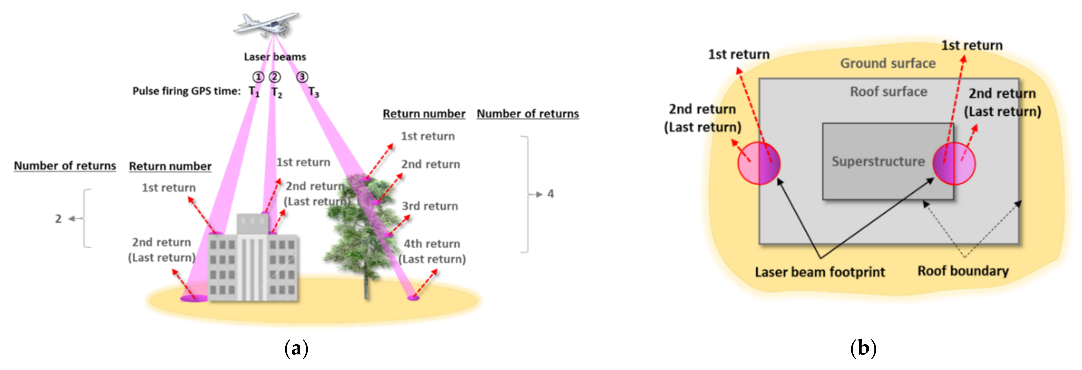
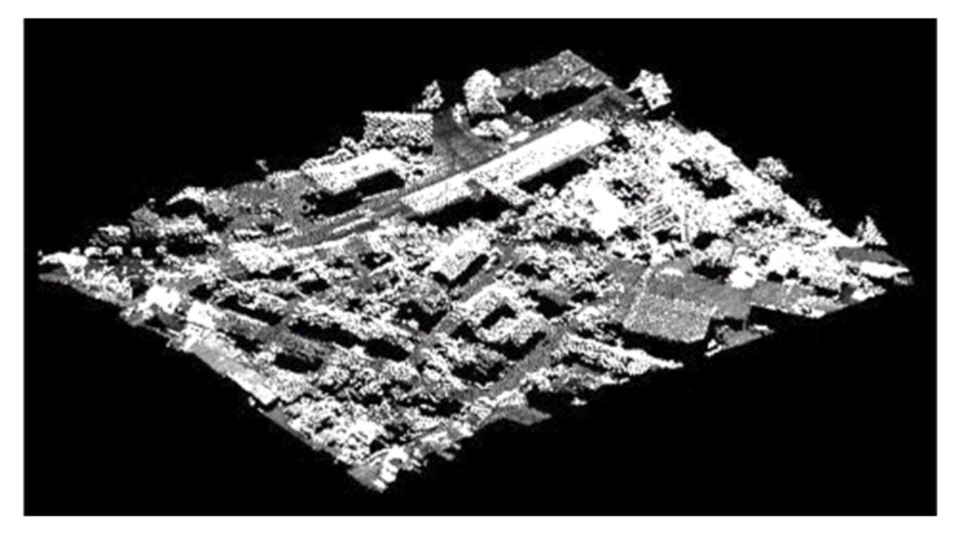
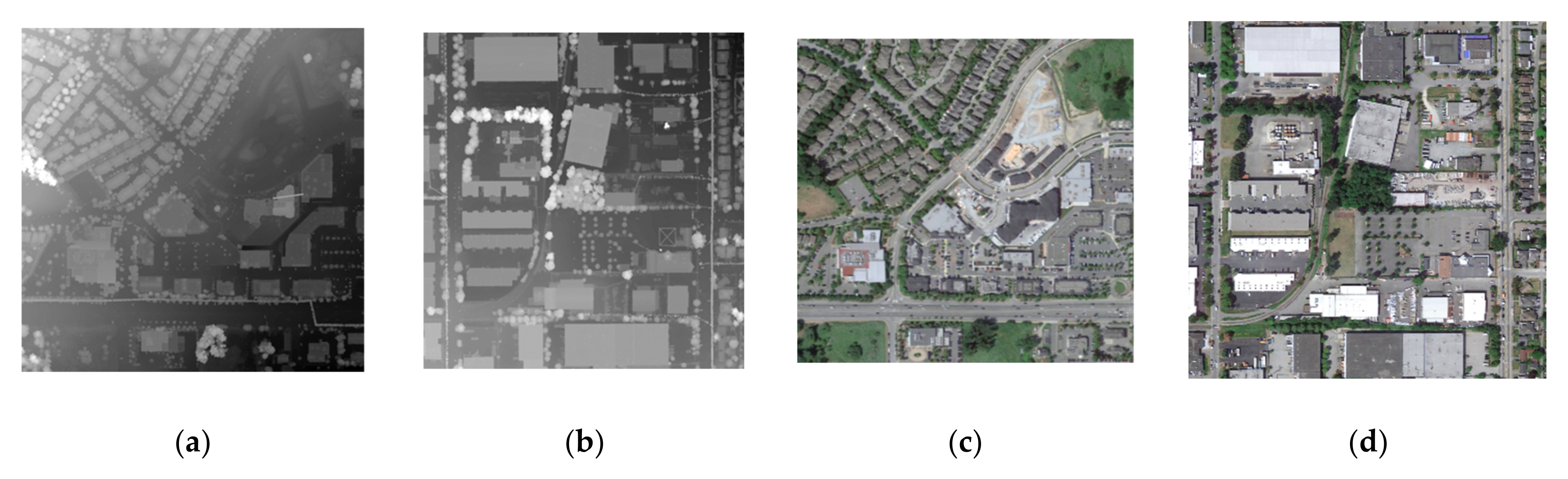
2.1.1. DALES Datasets

The DALES dataset is a large-scale aerial LiDAR dataset for point cloud segmentation. The objective of the DALES datasets is to help advance the field of deep learning within aerial LiDAR. The LiDAR data were collected using a Riegl Q1560 dual-channel ALS system over the City of Surrey in British Columbia, Canada. The LiDAR datasets have an average of 12 million points spanning a 10 km² area and contain 40 tiles (area of each tile is 500 × 500 m with a resolution of 50 pts/m² (ppm) and multiple return level of 7) of dense and labeled data with eight categories, namely, ground, vegetation, car, truck, pole, power line, fence, and building. The average ground sample distance (GSD) is approximately 0.15 m. The mean error was determined to be ±8.5 cm at 95% confidence level for the vertical accuracy [16,17,18].

The DALES datasets were used to train the PointNet++ model and test for the performance of the model. Figure 2 shows locations of 40 tiles of DALES datasets. Figure 3 shows 29 training and 11 test datasets that were fed to PointNet++. Figure 4 depicts the LiDAR data and color-labeled land cover classes. Figure 5 is a 3D perspective view of the LiDAR data.

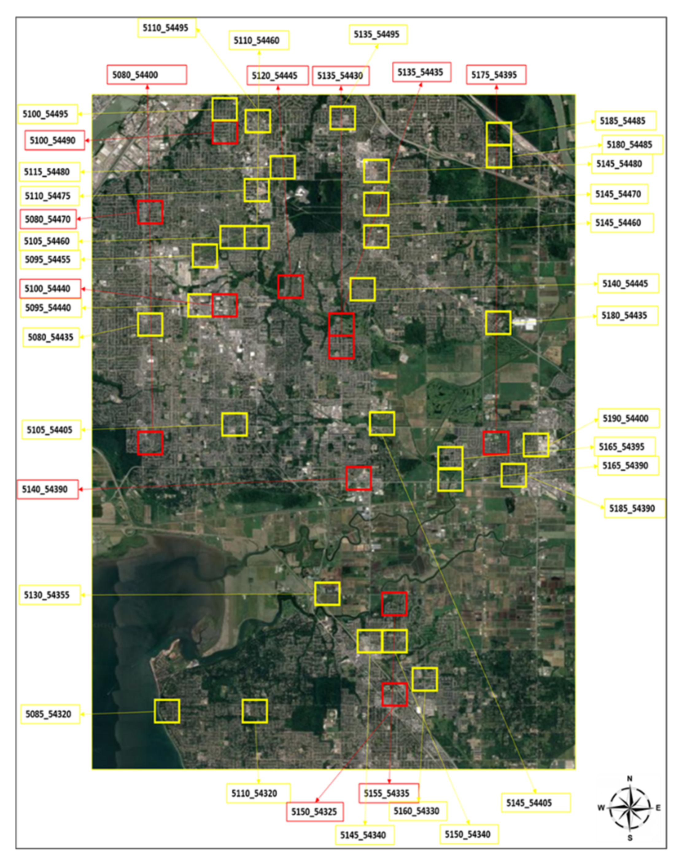
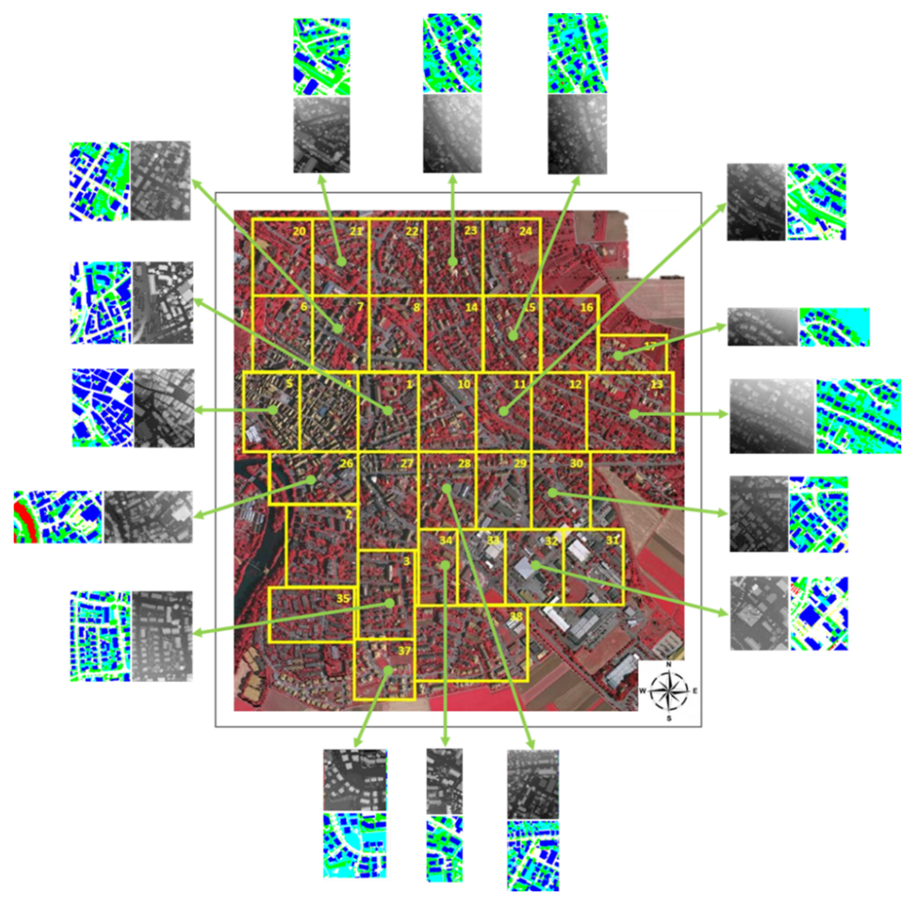
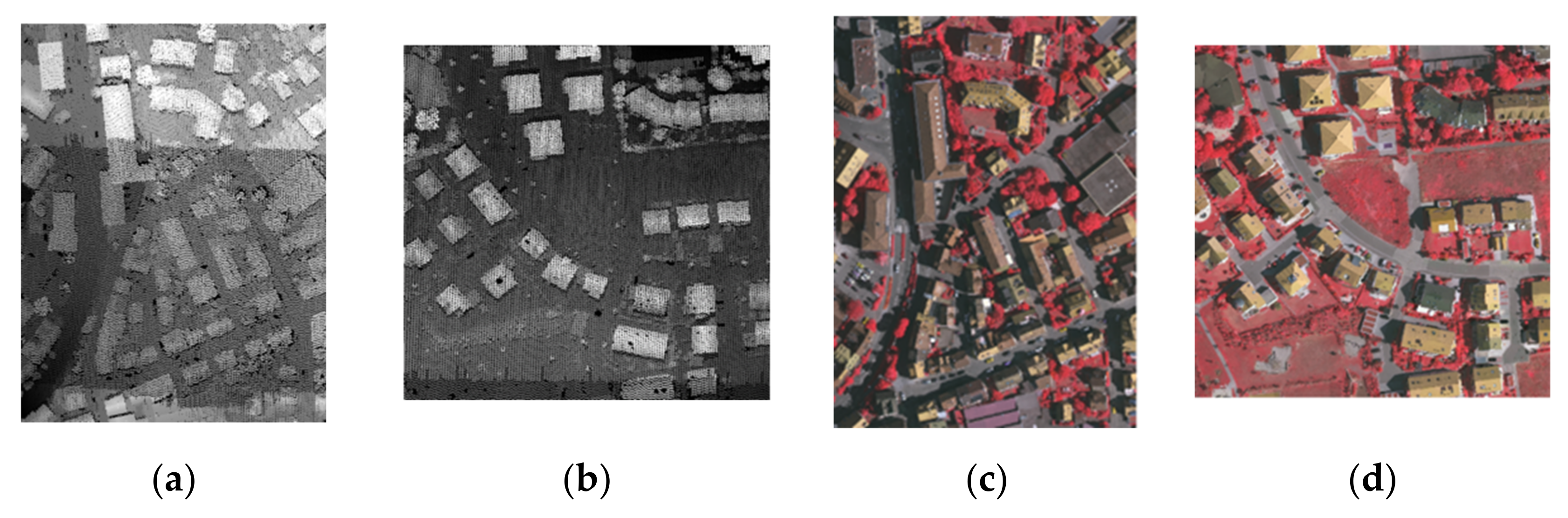
2.1.2. ISPRS Vaihingen Datasets

The ISPRS Vaihingen datasets, which are provided by the German Society for Photogrammetry, Remote Sensing and Geoinformatics, are for object classification and building reconstruction. The LiDAR data of the Vaihingen in Germany was acquired using a Leica ALS50 sensor (Leica Geosystems, Heerbrugg, Switzerland). The LiDAR point density varies between 4 and 7 ppm that is equivalent to GSD of 0.4 m–0.5 m. The datasets include IR aerial true orthoimages and DSMs with resolution of 0.09 m (Figure 6). Furthermore, they also include label data of geo-coded land cover classification with six classes, namely, impervious surface, building, low vegetation, tree, car, and clutter/background, as shown in Figure 7 [19,20,21]. Figure 8 is 3D perspective view of the LiDAR data.

The standard LiDAR data format is LAS (i.e., LASer file format). The LAS specification was developed and is maintained by the American Society for Photogrammetry and Remote Sensing (ASPRS). The LAS format includes 3D coordinates (i.e., X, Y, and Z) of each point, and additional attributes are provided: intensity, return number, number of returns, classification values, edge of flight line, RGB values, GPS time, scan angle, and scan direction.

Table 1. Example of return number and number of returns of LiDAR data.

Laser Beam	X	Y	Z	Return Number	Number of Returns
①	514,519.07	5,447,023.33	95.39	1	2
	514,520.24	5,447,031.85	91.71	2	2
②	514,519.10	5,447,023.81	96.14	1	2
	514,520.23	5,447,023.02	95.26	2	2
③	514,519.13	5,447,023.63	100.20	1	4
	514,519.33	5,447,024.32	97.76	2	4
	514,519.41	5,447,024.63	96.76	3	4
	514,519.65	5,447,025.46	92.81	4	4

shows an example of the return number and number of returns of the LiDAR data in LAS format (see Figure 1).

In this paper, the number of return attributes plays a crucial role in extracting buildings. Two returns of the LiDAR data with the LAS format are dominantly generated along the building boundaries. “Return number” and “number of returns” are confused frequently. An emitted laser pulse can have several returns depending on the features it is reflected from and the capabilities of the laser scanner used to collect the data. The first return will be flagged as return number one, the second as return number two, and so on, with the LAS format. On the other hand, the number of returns is the total number of returns for a given pulse. For example, a laser point may be return two (i.e., return number) within a total number of returns [22].

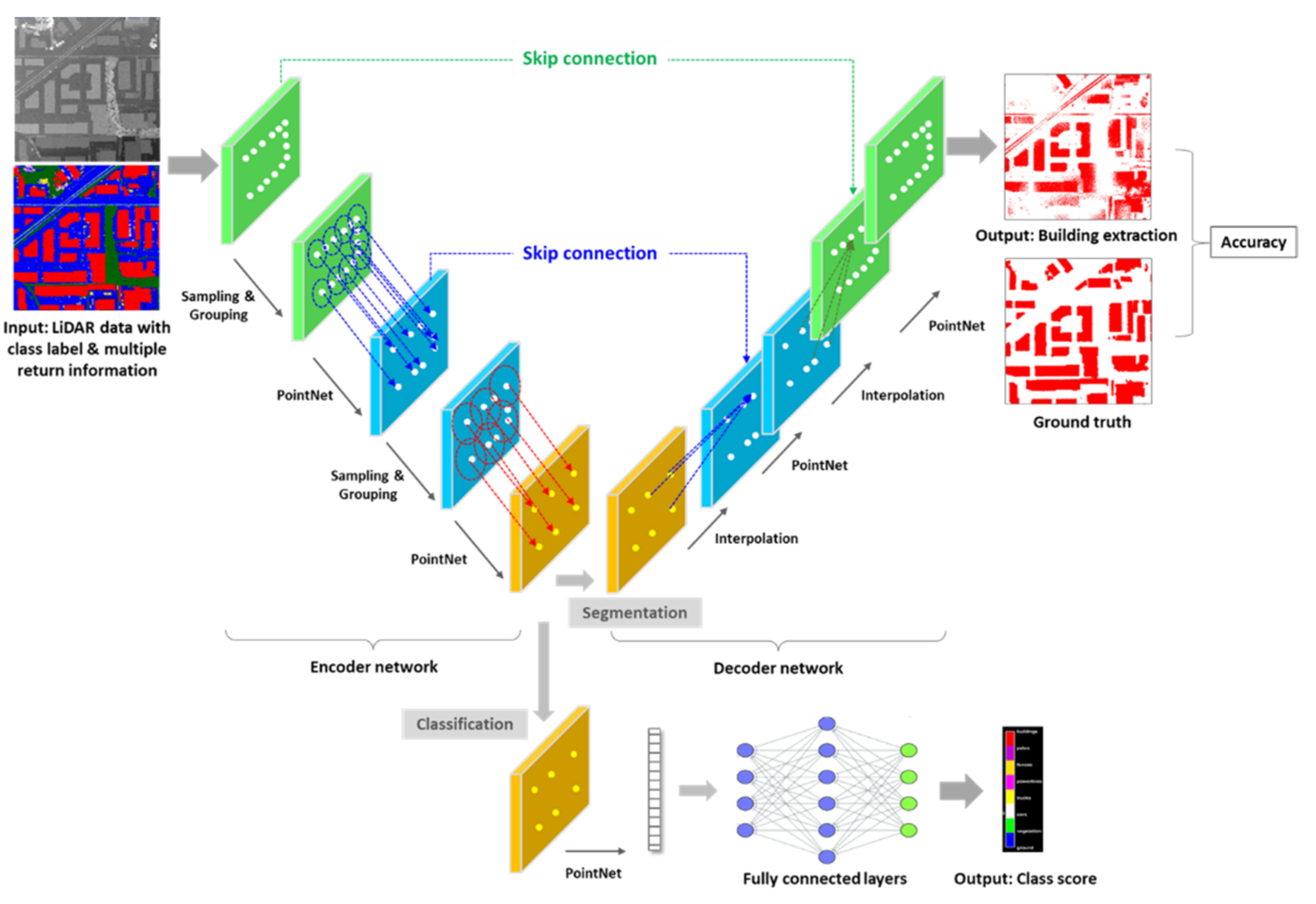
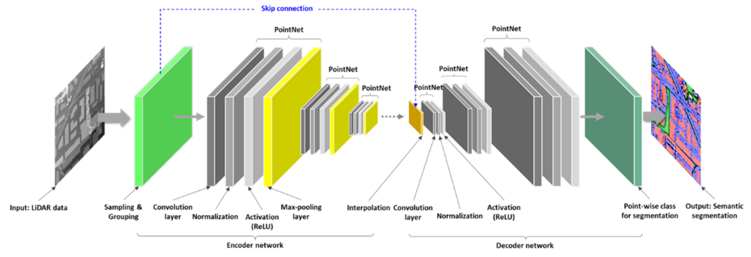
2.2. Overview of PointNet++ Model

PointNet++ is recognized as a state-of-the-art DL model and superior to other DL models for semantic segmentation and classification using point cloud data. PointNet++ is an improved DL version of the PointNet since PointNet does not extract the local features of the point clouds successfully [9]. The PointNet++ is a hierarchal network applying recursive PointNet for partitioned point clouds to capture fine-grained patterns in the data for classification and semantic segmentation. In PointNet++, the farthest point is selected for the given point cloud sets to form centroids for determining nearest neighbor points for each centroid. Then, the PointNet is applied to the local regions to generate a feature vector for each region [23]. PointNet++ adopts the U-Net architecture using skip link concatenation (or skip connection) [24].

The set-abstraction levels within the encoder network of PointNet++ are composed of sampling, grouping, and PointNet layer. The PointNet compoment contains a set of convolution, normalization, and rectified linear units (ReLU) followed by a max-pooling layer. The feature vectors are created from the local region patterns during the encoding process. On the other hand, the decoder network is composed of interpolation and PointNet layer. Figure 9 represents the architecture of PointNet++, and Figure 10 illustrates the PointNet configuration in the PointNet++ model.

The sampling layer selects a set of points that can define the centroids of local regions through selecting a subset of the farthest points to each other from the point clouds. The grouping layer organizes local regions by searching neighboring points around the centroids. Then, the subsampled data are fed to the PointNet for encoding the local region patterns into the feature vectors. By stacking several set abstraction levels, PointNet++ can learn features from a local geometric structure and abstract the local features layer by layer [5]. Details of PointNet++ including multi-scaling grouping and multi-resolution grouping that are to solve point data with non-uniform density efficiently are described in [25,26].

2.3. Proposed Scheme and Experiments

A total of 29 data tiles out of 40 tiles from the DALES datasets were used for training of PointNet++. Test of the trained PointNet++ was performed with the remaining 11 tiles. In addition to tests with DALES datasets, another test was performed with new data from the ISPRS Vaihingen datasets. The ultimate goal of DL is to generalize the trained models. In other words, ability of the models to adapt properly to new data is critical to achieving generalization (versatility or universality) of DL. Tests using data similar to the training datasets (i.e., data selected from the same region) could not refer to evaluation of DL models. In this respect, ISPRS Vaihingen datasets were chosen as the new data. To improve capturing the local features, we partitioned the training data tiles with size of 500 × 500 m into 50 × 50 m sub-areas because various objects could be mixed in the larger areas, leading to decreased training performance. Data partitioning not only increases the amount of data but also improves uniqueness and diversification of the data that are requirements of the training data for DL models.

The experiments for the semantic segmentation were performed using PointNet++ with airborne LiDAR data of the DALSE and ISPRS Vaihingen datasets. PointNet++ is one of the successful point-based DL models for semantic segmentation by training unorganized 3D point cloud data. The PointNet++ model consists of partitioning point clouds and extracting features. The model applies previously developed PointNet recursively to extract multi-scale features for accurate semantic segmentation [27]. The main tasks of using airborne LiDAR data in the field of photogrammetry are spatial database building, topographic mapping, DSM generation, 3D object reconstruction and modeling, and 3D city modeling for digital twin. Recently, deep learning solutions are increasingly involved in accomplishing these tasks. To improve performance of the DL model, one can add the number of return additional attributes (or additional features) to the training data. Figure 11 shows the workflow of the proposed method.

Figure 12 and Figure 13 show the characteristics of the two returns, and these datasets were used for evaluating the proposed method. It is clear that the two returns dominantly conveyed building boundaries. If LiDAR data with two returns is utilized, it is particularly beneficial to identify and extract buildings. The quality of the DALES datasets is superior to the ISPRS Vaihingen datasets in terms of the point density. Moreover, the quality of the LiDAR data depends on the performance of the laser sensor. Therefore, points with two returns in DALES datasets represent much clearer building boundaries formed by two returns than ISPRS Vaihingen datasets. The experiments showed that the quality of the points on the building boundaries affect building segmentation.

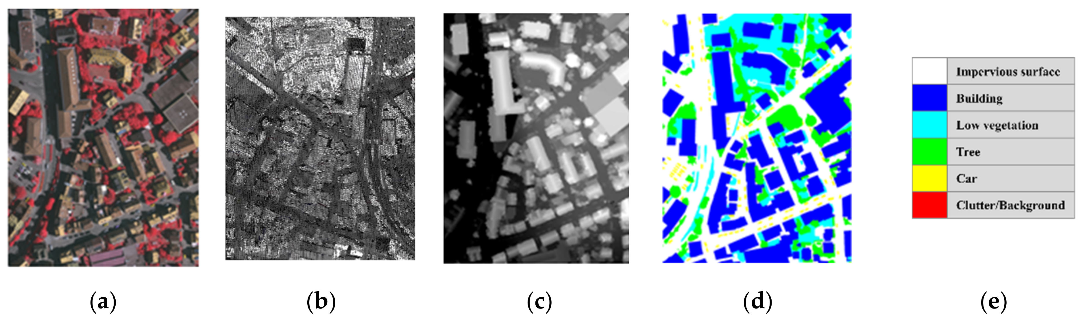
2.4. Accuracy Assessment

In general, the performance of deep learning is based on the evaluation metrics such as accuracy and loss of the DL model training, IoU, recall, F1-score, confusion matrix, etc. Since such metrics are statistical representations of the overall quality by quantitative numbers computed using formal equations, there is a limitation in revealing the local and detailed phenomena. In this regard, visualization of the differences between prediction and ground truth leads to meaningful evaluation and analysis of the results. In particular, the pattern and location of the misclassified features can be identified through visual inspection on the basis of the difference images between prediction and ground truth.

We applied global accuracy (or overall accuracy (OA)), mean accuracy, mean intersection-of-union (mIOU), weighted IoU, IoU, and recall to evaluate DL model training performance and results of the semantic segmentation. Mean accuracy is the average accuracy of all classes in particular data (i.e., each test and new data). Weighted IOU is for reducing the impact of errors in the small classes by taking number of points into account for each class. The evaluation metrics are as follows:

$$Global accuracy=\frac{Number of correct prediction}{Total number of prediction}=\frac{TP+TN}{TP+TN+FP+FN}$$

(1)

$$Mean accuracy=\frac{\sum \left(each class accuracy\right)}{k}$$

(2)

$$IoU=\frac{Area of overlap}{\mathrm{Area} \mathrm{of} \mathrm{union}}=\frac{Area \left(prediction \cap target\right)}{Area \left(prediction \cup target\right) }=\frac{TP}{TP+FP+FN}$$

(3)

$$mIoU=\frac{1}{k+1}{\displaystyle \sum }_{i=0}^k\frac{TP}{TP+FN+FP}$$

(4)

$$Recall=\frac{TP}{TP+FN}$$

(5)

where TP, TN, FP, and FN are true positive, true negative, false positive, and false positive, respectively. k is number of classes.

Class imbalance is a common problem in deep learning for multi-class classification or segmentation with a disproportionate ratio of the data in each class. i.e., there is a significant discrepancy in the amount of data across different classes. In this case, the prediction accuracy of the class with greater data is higher than that of the class with less data. Therefore, the ideal case would be for each class to have approximately the same amount of data [28,29].

We applied weighted cross-entropy loss among the approaches for correcting class imbalance such as over- or under-sampling, class aggregation, class weighting, focal loss, and incremental transfer learning. The concept of the weight-based class imbalance correction is that the weights are assigned inversely proportional to the number of data of the classes. The weighted cross-entropy weights the losses associated with incorrectly predicting rarer data more heavily than losses associated with more data as follows [30]:

$$w \left(p, y\right) = {\displaystyle \sum }_{t=1}^C{w}_t p_t log \left(y_t\right)$$

(6)

where p_t and y_t denote the probability estimate and ground truth of class t, respectively. C denotes the number of ground truth classes, and w_t denotes the weight for class t.

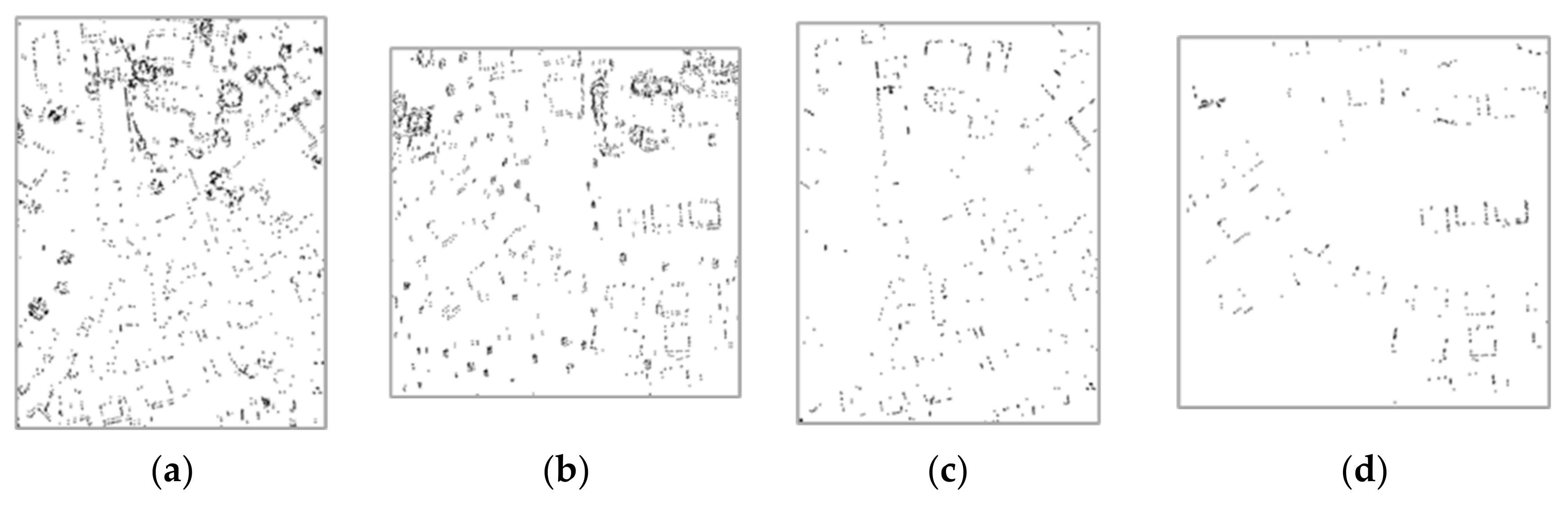
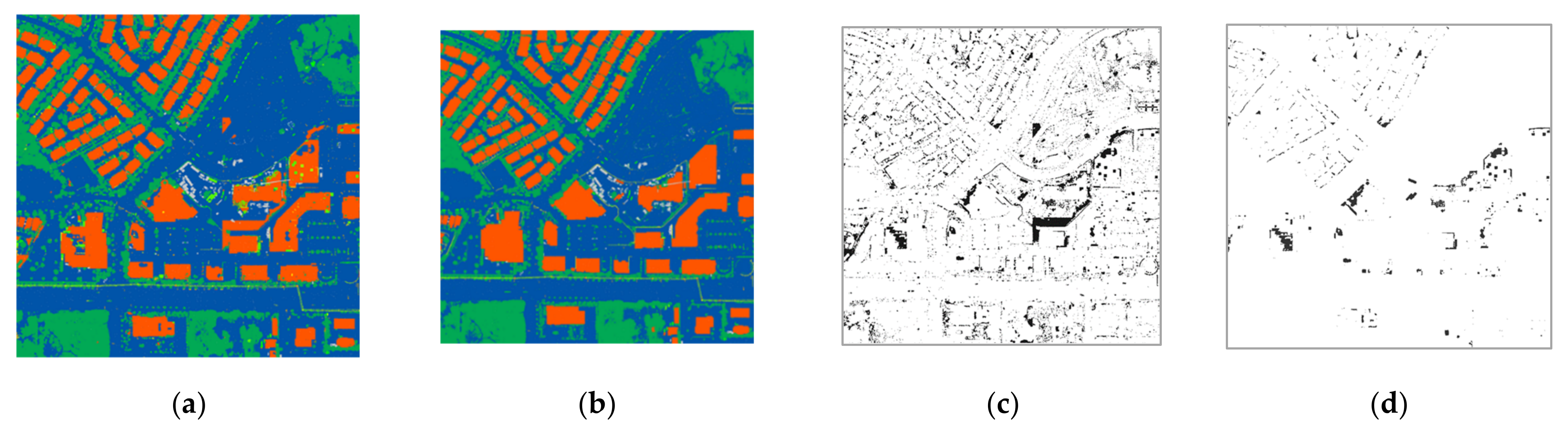
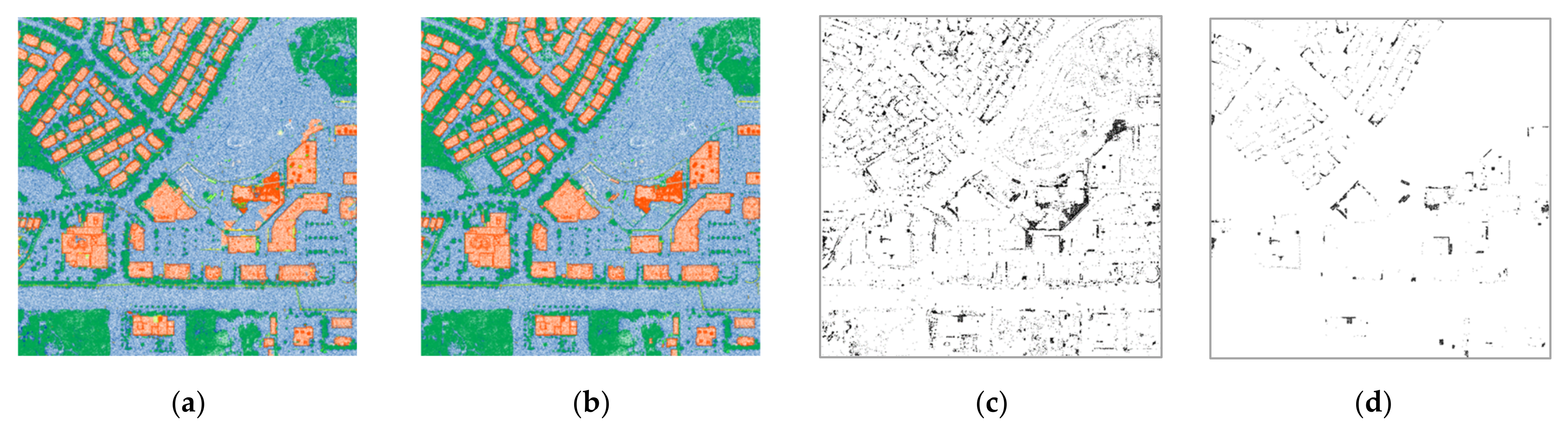
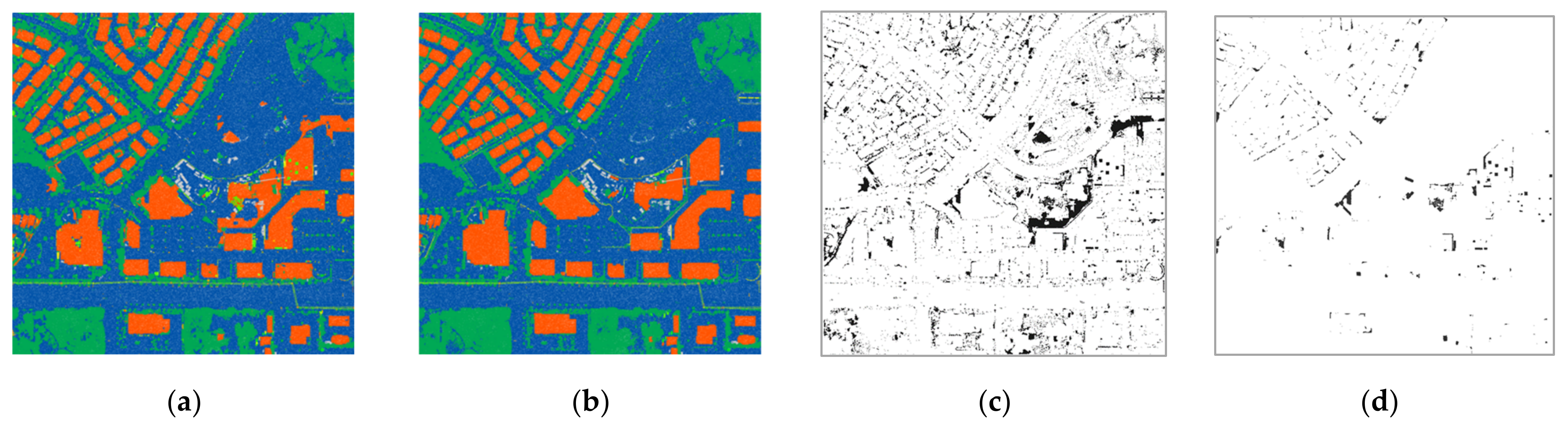
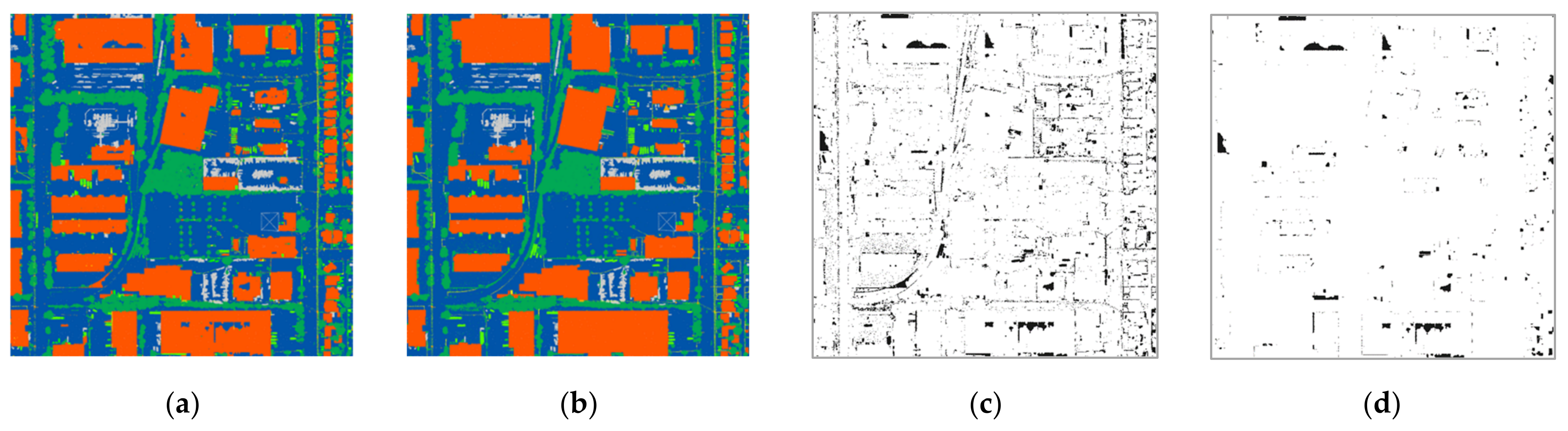
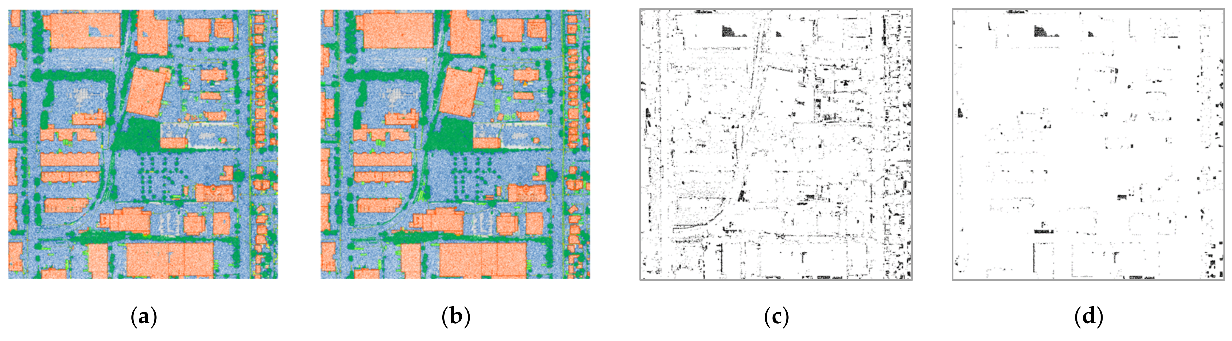
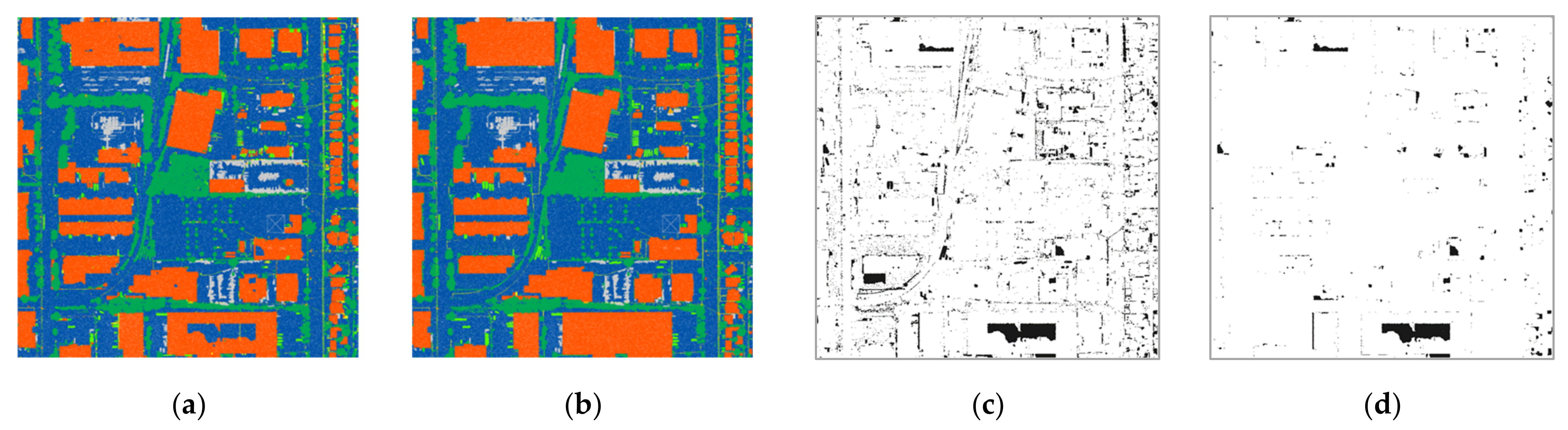
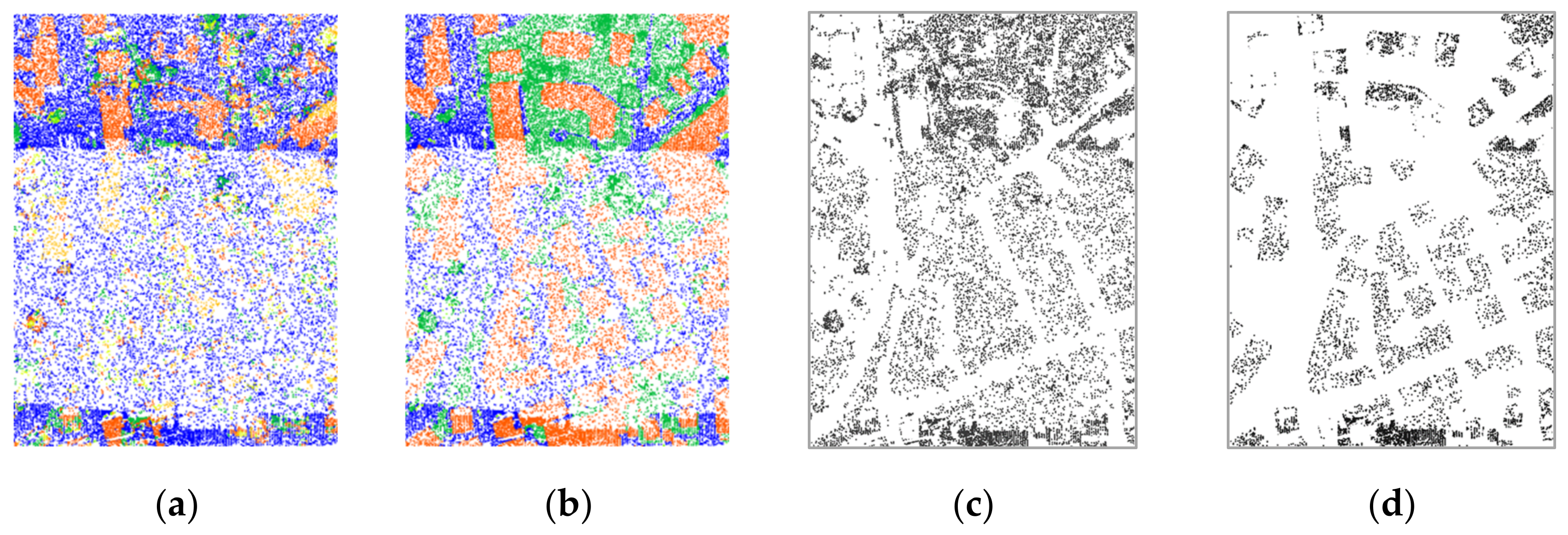
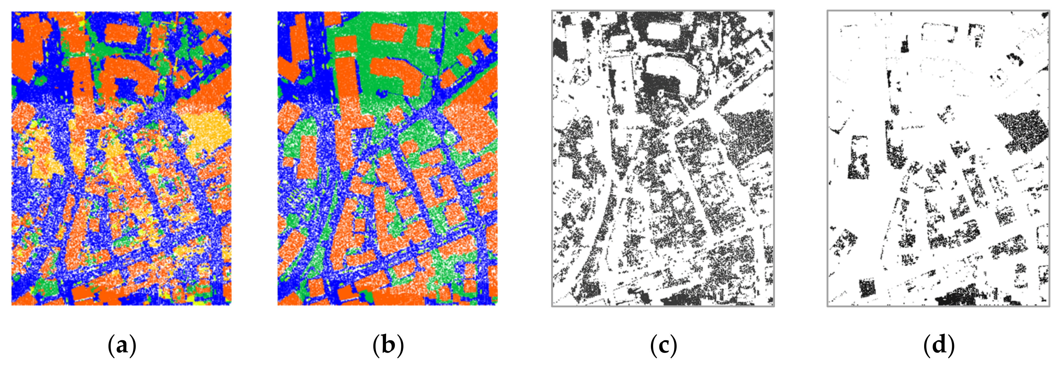
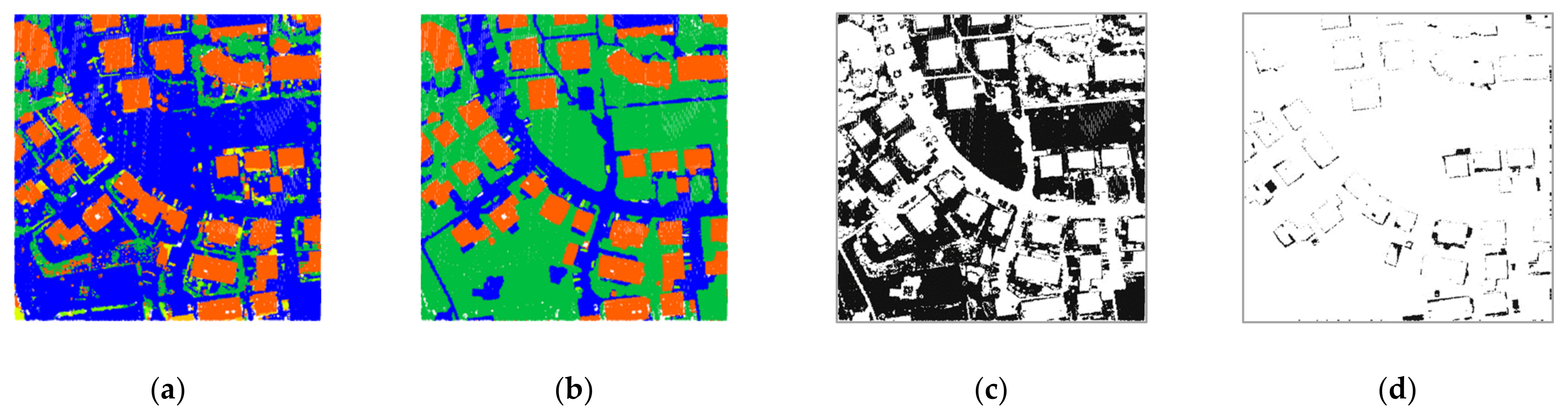
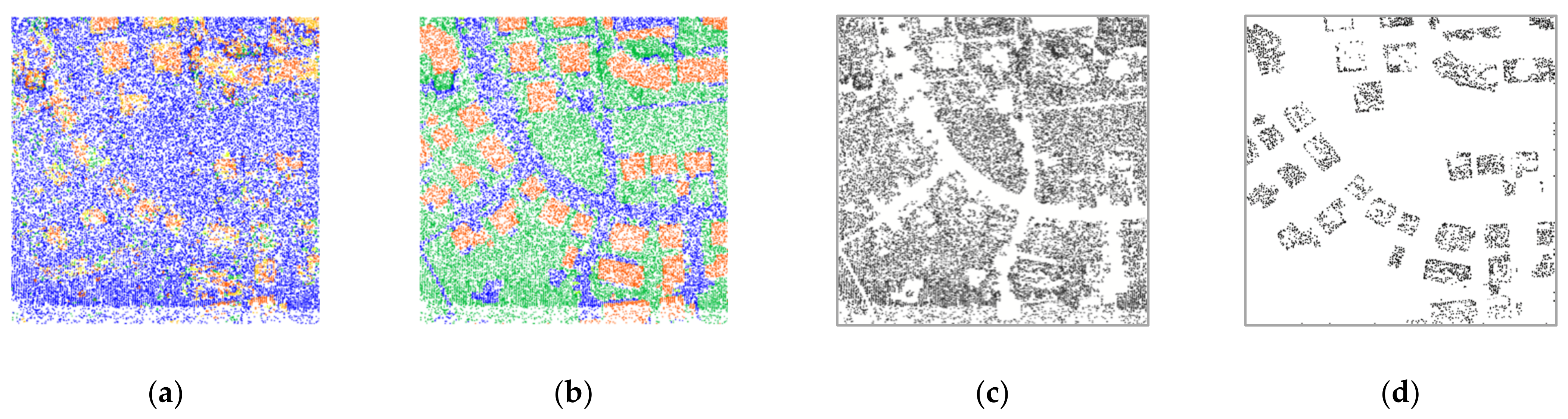
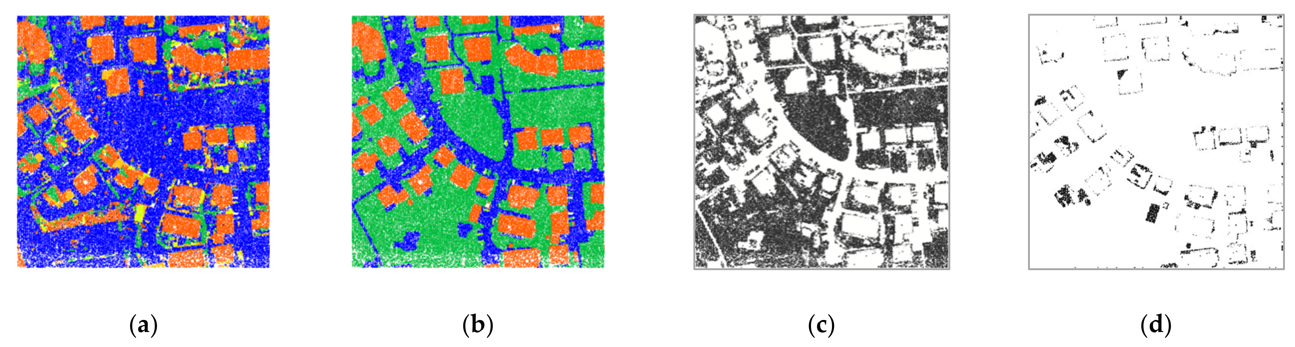
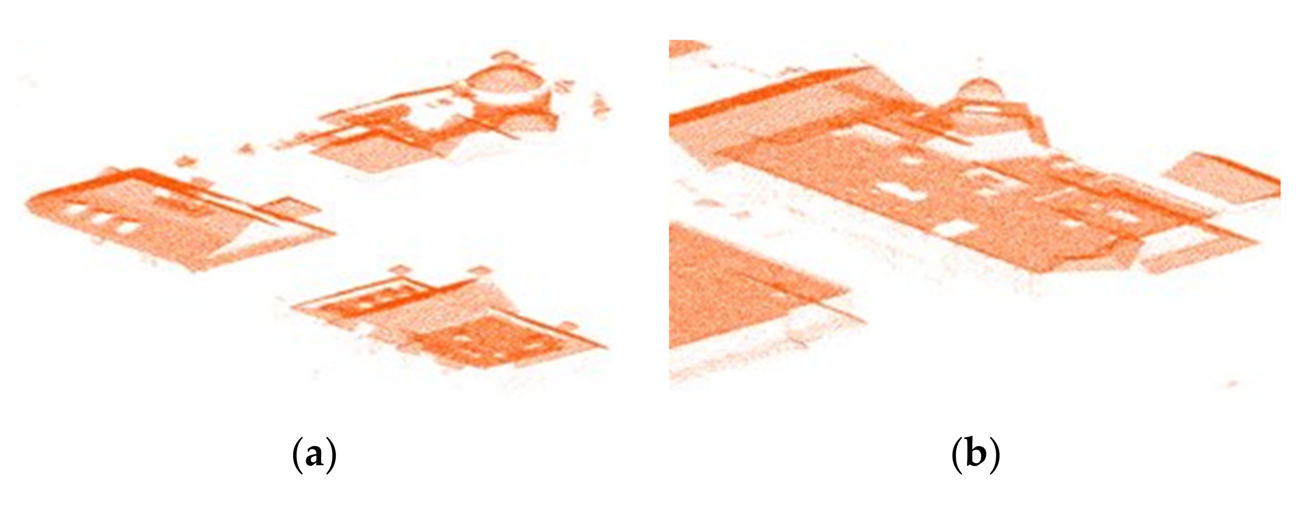
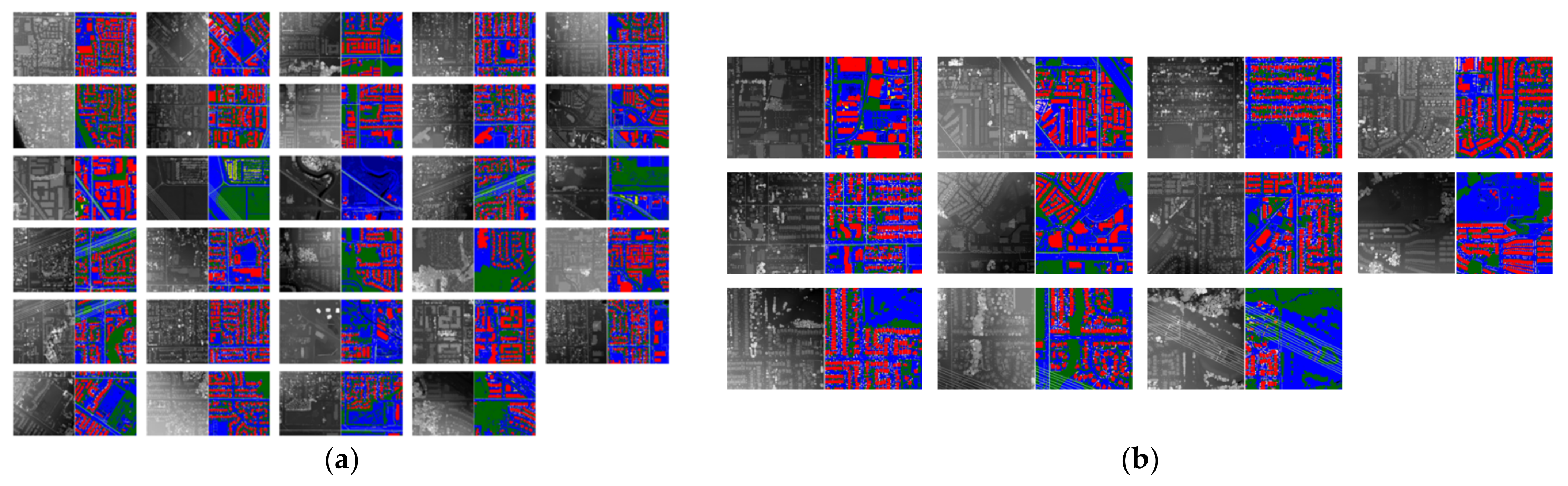
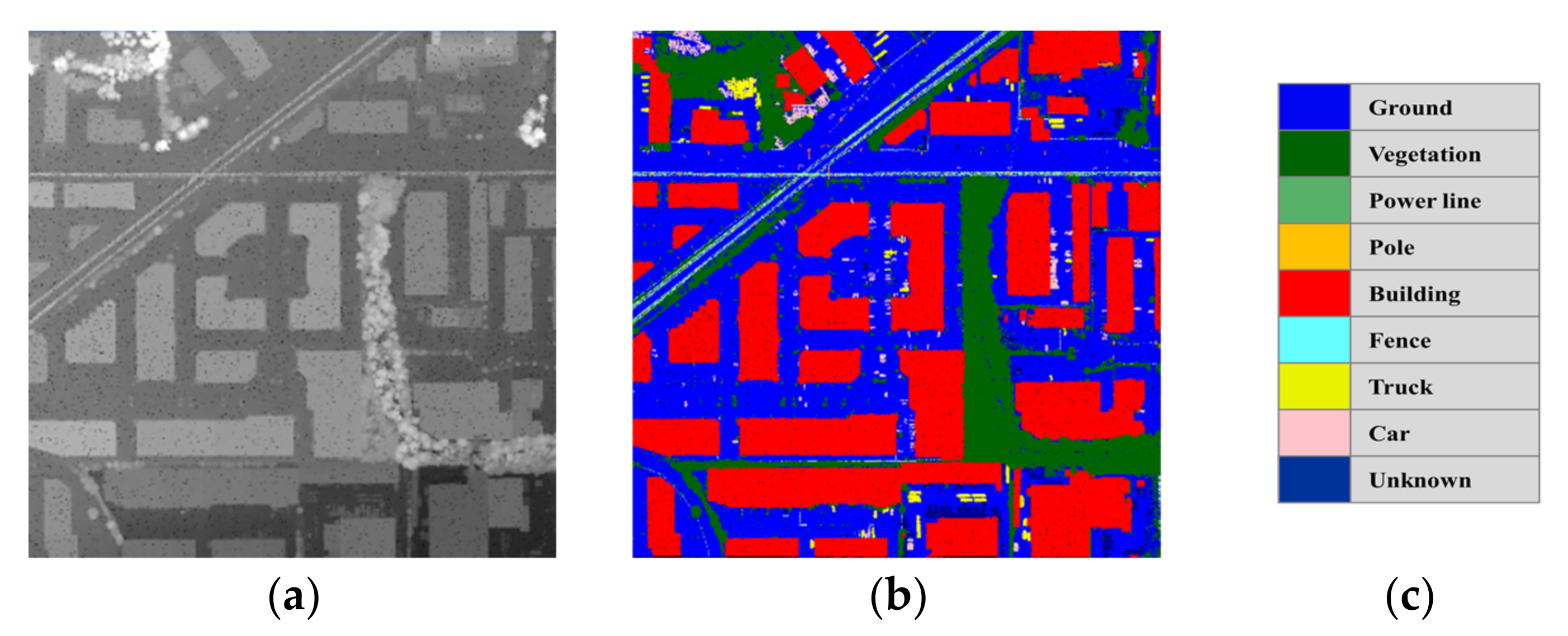
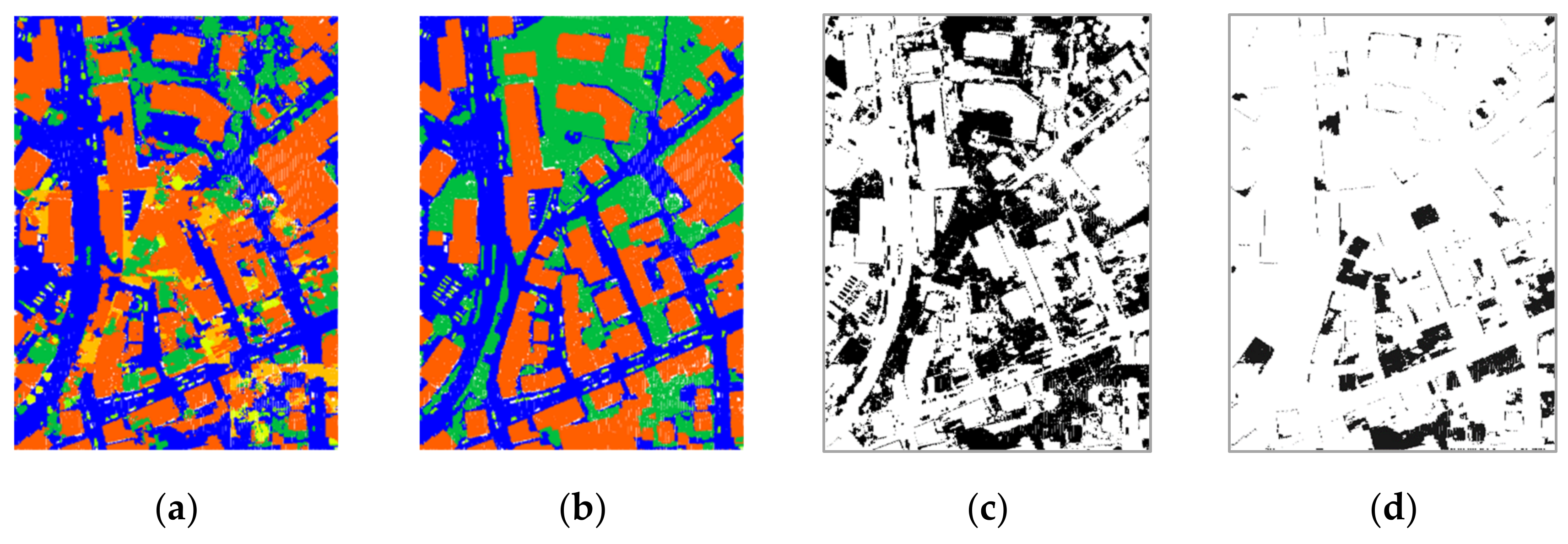
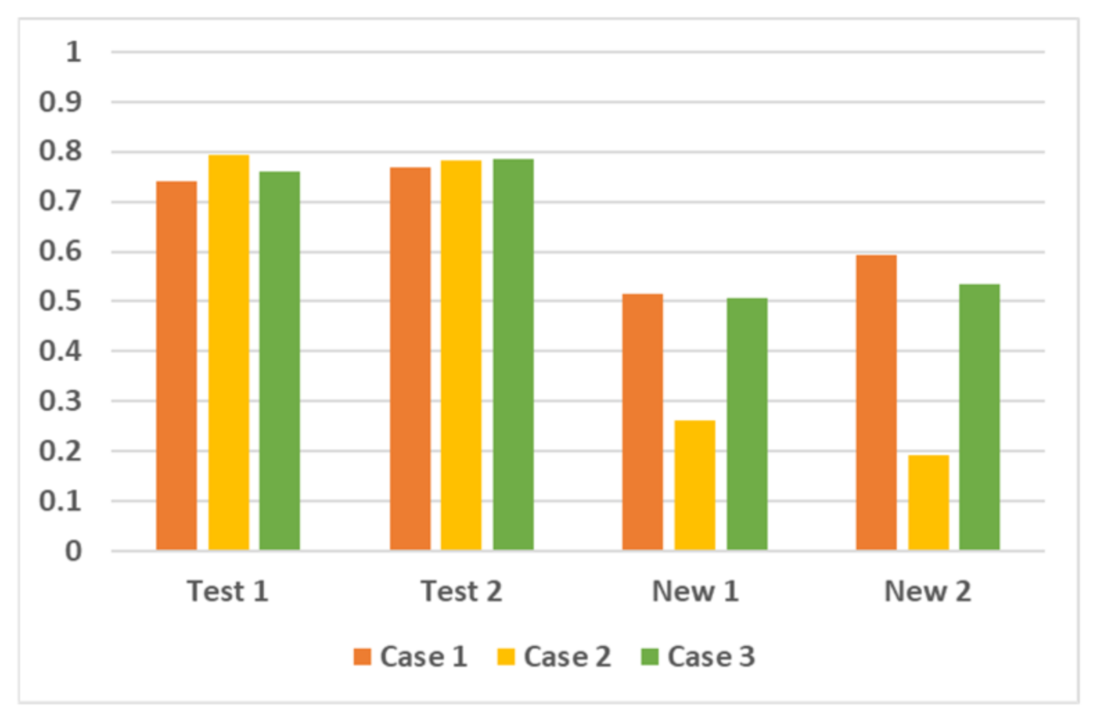
3. Experimental Results and Analysis

Two LiDAR data were selected from the DALES datasets as test data, and two LiDAR data were selected from the ISPRS Vaihingen datasets as new data. The test and new data are shown in Figure 14 and Figure 15, respectively. The aerial images in Figure 14 were captured from Google Earth since images were not included in the DASLES datasets. The aerial IR images were provided by ISPRS Vaihingen datasets. Even though the aerial images were not involved in training PointNet++, they are presented for the purpose of identifying regional characteristics and visually analyzing semantic segmentation results. The parameters for training PointNet++ were that training epoch was 20, mini-batch size was 6, and learning rate started from 0.0005 for the first 10 epochs then 0.00005 after 10 epochs. Results of the semantic segmentation from following cases are presented:

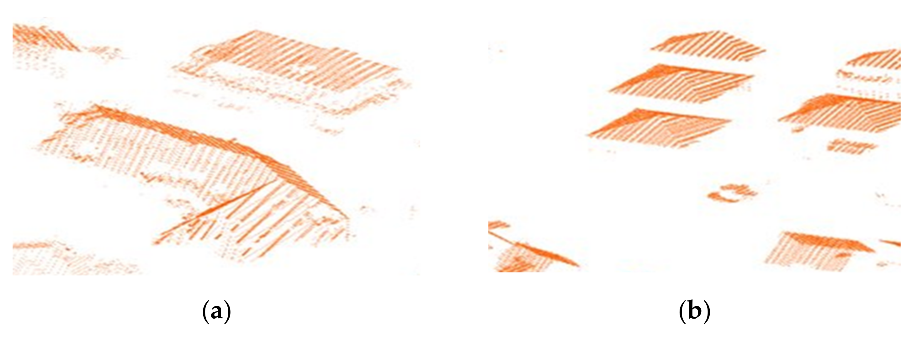
• Case 1: Original datasets (i.e., all number of returns)
• Case 2: Datasets of two returns with randomly selected points of 10% from the original datasets
• Case 3: Datasets of two returns with randomly selected points of 50% from the original datasets

Figure 14. Test data from DALES datasets: (a) test LiDAR data 1; (b) test LiDAR data 2; (c) aerial image 1; (d) aerial image 2.

Figure 14. Test data from DALES datasets: (a) test LiDAR data 1; (b) test LiDAR data 2; (c) aerial image 1; (d) aerial image 2.

Figure 15. New data from ISPRS Vaihingen datasets: (a) new LiDAR data 1; (b) new LiDAR data 2; (c) aerial IR image 1; (d) aerial IR image 2.

Figure 15. New data from ISPRS Vaihingen datasets: (a) new LiDAR data 1; (b) new LiDAR data 2; (c) aerial IR image 1; (d) aerial IR image 2.

Figure 16, Figure 17, Figure 18, Figure 19, Figure 20, Figure 21, Figure 22, Figure 23, Figure 24, Figure 25, Figure 26 and Figure 27 show semantic segmentation results of test and new data from the trained PointNet++ model that was trained using DALES training datasets. The results in the figures consist of prediction from the model, ground truth (i.e., label data), visualization of difference between prediction and ground truth, and the difference for buildings only. Black and while areas in the difference images indicate misclassified and correctly classified LiDAR points, respectively. Most of the erroneous results (i.e., black areas in the difference images) occur at the objects’ edges (or boundaries). These might be caused from the hand-labeling process because identification of each point is a challenging task, especially for the ambiguous or unclear boundaries between adjacent objects. Moreover, the sampling, grouping, and interpolation in the PointNet++ could affect the errors between prediction and ground truth. Therefore, errors are more clearly visible at the boundaries of the objects.

Figure 28 and Figure 29 depict 3D perspective views of the point clouds belonging to the building class of the DALES test data and ISPRS Vaihingen new data, respectively. The building points were extracted from the semantic segmentation results by applying the proposed methods.

Training accuracy alone is not sufficient in determining the performance of the models since it is not always representative of each class within the datasets. It is more important to assess the robustness and generalization of a DL model for the new datasets since the ultimate goal of DL is to expand the trained model to other datasets (i.e., new or unseen data) that are not involved with training. On the other hand, IoU is calculated for each class separately, then averaged over all classes to provide the mIoU score of semantic segmentation prediction. The threshold to be considered accpetable prediction is 0.5. If IoU is larger than 0.5, it is normally considered a good prediction [15,31]. The results show that LiDAR data with two returns and appropriate point density could lead to improved results on the building boundaries.

In order to assess the proposed method, we analyzed results from each case for the test and new data on the basis of the visual inspection as well as standard evaluation metrics. Performance of the DL model training is presented in

Table 2. Training accuracy and loss for each case.

Evaluation Metrics	Case 1	Case 2	Case 3
Accuracy (%)	97.08	95.55	96.45
Loss	0.20	0.23	0.20

in terms of accuracy and loss. The overall evaluation of the trained model is shown in

Table 3. Evaluation metrics of test and new data for each case.

Dataset	Evaluation Metrics	Case 1	Case 2	Case 3
Test 1	Global accuracy	0.9253	0.8869	0.9126
	Mean accuracy	0.6254	0.6304	0.6323
	Mean IoU	0.4287	0.4640	0.4474
	Weighted IoU	0.8669	0.8017	0.8454
Test 2	Global accuracy	0.9399	0.9059	0.9281
	Mean accuracy	0.6411	0.6640	0.6537
	Mean IoU	0.4979	0.5284	0.5031
	Weighted IoU	0.8937	0.8372	0.8738
New 1	Global accuracy	0.6557	0.4754	0.6349
	Mean accuracy	0.5216	0.3952	0.4961
	Mean IoU	0.1916	0.1261	0.1860
	Weighted IoU	0.4958	0.3115	0.4781
New 2	Global accuracy	0.5064	0.3104	0.4656
	Mean accuracy	0.4976	0.3344	0.4630
	Mean IoU	0.1591	0.0768	0.1405
	Weighted IoU	0.3475	0.1540	0.3011

with accuracy and IoU. Classification accuracy of each class is shown in

Table 4. Classification accuracy of test and new data.

Dataset	Class	Accuracy			IoU
		Case 1	Case 2	Case 3	Case 1	Case 2	Case 3
Test 1	Ground	0.9740	0.9607	0.9659	0.9140	0.8462	0.8955
	Vegetation	0.8663	0.8528	0.8610	0.8035	0.7909	0.7986
	Car	0.4005	0.3804	0.3980	0.2615	0.2837	0.2822
	Truck	0.3731	0.1300	0.2562	0.0236	0.0198	0.0207
	Powerline	0.8661	0.8703	0.8731	0.3932	0.5568	0.4650
	Fence	0.0498	0.2979	0.1993	0.0391	0.1872	0.1136
	Pole	0.5767	0.7089	0.6230	0.1413	0.2527	0.1825
	Building	0.8966	0.8420	0.8820	0.8537	0.7747	0.8208
Test 2	Ground	0.9924	0.9898	0.9874	0.9302	0.8964	0.9166
	Vegetation	0.8826	0.8651	0.8773	0.8445	0.8147	0.8355
	Car	0.6838	0.3482	0.5332	0.2060	0.1711	0.2196
	Truck	0.4217	0.4077	0.3738	0.2750	0.3033	0.2431
	Powerline	0.6757	0.7863	0.7677	0.5517	0.6407	0.5376
	Fence	0.1207	0.5763	0.3530	0.0907	0.2999	0.1816
	Pole	0.4210	0.4619	0.4332	0.1788	0.2546	0.2108
	Building	0.9208	0.8764	0.9044	0.9067	0.8464	0.8797
New 1	Ground	0.8814	0.9046	0.8534	0.5666	0.4129	0.5556
	Vegetation	0.3350	0.2296	0.2831	0.2838	0.2098	0.2515
	Car	0.1852	0.0756	0.1270	0.0920	0.0517	0.0953
	Building	0.7523	0.3712	0.7208	0.6573	0.3342	0.5858
New 2	Ground	0.9445	0.9570	0.9429	0.3292	0.2742	0.3299
	Vegetation	0.1712	0.0583	0.1332	0.1680	0.0564	0.1298
	Car	0.0237	0.0139	0	0.0588	0.0085	0
	Building	0.8512	0.3086	0.7760	0.7699	0.3797	0.6644

. It was noticed that land cover class of DALES and ISPRS Vaihingen datasets were not the same, as shown in Figure 4c and Figure 7e. Therefore, the classes in test data and new data did not coincide with each other.

The major objective of the proposed method was in utilizing multiple returns of the LiDAR data. Specifically, two returns of the laser pulse convey rich information of the building boundaries. In consequence, the accuracy of the building boundaries for the test data in terms of recall were improved by utilizing two returns, as shown in

Table 5. Recall of building boundaries.

Dataset	Case 1	Case 2	Case 3
Test 1	0.7417	0.7948	0.7598
Test 2	0.7691	0.7826	0.7851
New 1	0.5158	0.2611	0.5063
New 2	0.5938	0.1930	0.5344

and Figure 30. However, there was not significant improvement for the new data because of the poor quality of the new data (i.e., 4~7 ppm) caused by low point density compared with the training datasets (i.e., 50 ppm).

4. Conclusions and Discussion

Extraction of building data consisiting of 3D information is important for building modeling since 3D building models are utilized in various applications such as 3D mapping, city modeling and planning, and smart city associated with digital twin. LiDAR data contain not only spatial information but also unique attribute information. In particular, multiple returns of the laser beams imply the geometric characteristics of objects. The proposed method aims to accurately extract point clouds belonging to buildings by preserving the structual boundaries on the basis of the number of returns. The results of this study could be used to process 3D building modeling.

Utilizing two returns yielded higher recall values of the building boundaries for the test data. The maximum improvement was from 0.7417 to 0.7948 for test data 1, and 0.7691 to 0.7851 for test data 2 in terms of recall value. However, there was no significant improvement for the new data. The quality and characteristics of the test and new data should be similar to the training data of the DL model for optimal results. Therefore, the results of the new data were not satisfactory because the quality of the data was lower than that of the training data. However, buildings were adequately identified and classified compared to the other objects.

In consequence, it is not sufficient to successfully carry out the semantic segmentation of real-world objects by the raw (of original) data only. Additional meaningful attribute and intrinsic information in the data could improve the performance for achieving objectives. In this respect, multi-source and multi-modal data are being utilized more frequently. In this regard, it is valuable to implement attributes such as multiple return information of LiDAR data.

In addition, multiple return of the LiDAR could be applied to extract specific features. For example, trees generate more multiple returns than other objects. Therefore, in order to extract trees from the LiDAR data and create a 3D forest map for use in environmental and ecosystem research, one must classify trees. By using multiple returns, one can efficiently identify and distinguish trees from other objects.

References

1. Maune, D. Digital Elevation Model Technologies and Applications: The DEM Users Manual, 2nd ed.; The American Society for Photogrammetry & Remote Sensing: Bethesa, MD, USA, 2007; pp. 199–424. [Google Scholar]
2. Shan, J.; Toth, C. Topographic Laser Ranging and Scanning: Principles and Processing; CRC Press: Boca Raton, FL, USA, 2009; pp. 403–573. [Google Scholar]
3. Beraldin, J.; Blais, F.; Lohr, U. Laser scanning technology. In Airborne and Terrestrial Laser Scanning; Vosselman, G., Maas, H., Eds.; CRC Press: Boca Raton, FL, USA, 2010; pp. 1–42. [Google Scholar]
4. Li, Y.; Ma, L.F.; Zhong, Z.L.; Liu, F.; Chapman, M.A.; Cao, D.P.; Li, J.T. Deep learning for LiDAR point clouds in autonomous driving: A review. IEEE Trans. Neural. Netw. Learn. Syst. 2021, 32, 3412–3432. [Google Scholar] [CrossRef] [PubMed]
5. Briechle, S.; Krzystek, P.; Vosselman, G. Semantic labeling of ALS point clouds for tree species mapping using the deep neural network PointNet++. Int. Arch. Photogramm. Remote Sens. Spat. Inf. Sci. 2019, 4213, 951–955. [Google Scholar] [CrossRef] [Green Version]
6. Lin, Y.P.; Vosselman, G.; Cao, Y.P.; Yang, M.Y. Local and global encoder network for semantic segmentation of airborne laser scanning point clouds. ISPRS J. Photogramm. Remote Sens. 2021, 176, 151–168. [Google Scholar] [CrossRef]
7. Meyer, G.P.; Laddha, A.; Kee, E.; Vallespi-Gonzalez, C.; Wellington, C.K. LaserNet: An Efficient Probabilistic 3D Object Detector for Autonomous Driving. In Proceedings of the 2019 IEEE/CVF Conference on Computer Vision and Pattern Recognition, Long Beach, CA, USA, 5–20 June 2019. [Google Scholar]
8. Hoang, L.; Lee, S.H.; Lee, E.J.; Kwon, K.R. GSV-NET: A multi-modal deep learning network for 3D point cloud classification. Appl. Sci. 2022, 12, 483. [Google Scholar] [CrossRef]
9. Qi, C.R.; Su, H.; Mo, K.; Guibas, L.J. PointNet: Deep Learning on Point Sets for 3D Classification and Segmentation. In Proceedings of the IEEE Conference on Computer Vision and Pattern Recognition, CVPR 2017, Honolulu, HI, USA, 16–21 July 2017. [Google Scholar]
10. Zaheer, M.; Kottur, S.; Ravanbhakhsh, S.; Póczos, B.; Salakhutdinov, R.; Smola1, A. Deep sets. NIPS 2017, 30. [Google Scholar]
11. Qi, C.R.; Yi, L.; Su, H.; Guibas, L.J. PointNet++: Deep Hierarchical Feature Learning on Point Sets in A Metric Space. In Proceedings of the Advances in Neural Information Processing Systems, Long Beach, CA, USA, 4–9 December 2017. [Google Scholar]
12. Guo, Y.; Wang, H.; Hu, Q.; Liu, H.; Liu, L.; Bennamoun, M. Deep Learning for 3D Point Clouds: A Survey. IEEE Trans. Pattern Anal. Mach. Intell. 2021, 43, 4338–4364. [Google Scholar] [CrossRef] [PubMed]
13. Audebert, N.; le Saux, B.; Lefèvre, S. Beyond RGB: Very high resolution urban remote sensing with multimodal deep networks. ISPRS J. Photogramm. Remote Sens. 2018, 140, 20–32. [Google Scholar] [CrossRef] [Green Version]
14. Maltezos, E.; Doulamis, A.; Doulamis, N.; Ioannidis, C. Building extraction from LiDAR data applying deep convolutional neural networks. IEEE Geosci. Remote Sens. Lett. 2019, 16, 155–159. [Google Scholar] [CrossRef]
15. Lee, D.G.; Shin, Y.H.; Lee, D.C. Land cover classification using SegNet with slope, aspect, and multidirectional shaded relief images derived from digital surface model. J. Sens. 2020, 2020, 8825509. [Google Scholar] [CrossRef]
16. Varney, N.; Asari, V.K.; Graehling, Q. DALES: A Large-scale Aerial LiDAR Data Set for Semantic Segmentation. In Proceedings of the IEEE/CVF Conference on Computer Vision and Pattern Recognition Workshops, Seattle, WA, USA, 14 April 2020. [Google Scholar]
17. Singer, N.M.; Asari, V.K. DALES Objects: A large scale benchmark dataset for instance segmentation in aerial Lidar. IEEE Access 2021, 9, 97495–97504. [Google Scholar] [CrossRef]
18. Dayton Annotated Laser Earth Scan (DALES). Available online: https://udayton.edu/engineering/research/centers/vision_lab/research/was_data_analysis_and_processing/dale.php (accessed on 22 August 2021).
19. Rottensteiner, F.; Sohn, G.; Jung, J.; Gerke, M.; Baillard, C.; Benitez, S.; Breitkop, U. The ISPRS benchmark on urban object classification and 3D building reconstruction. ISPRS Ann. Photogramm. Remote Sens. Spat. Inf. Sci. 2012, 1–3, 293–298. [Google Scholar] [CrossRef] [Green Version]
20. Cramer, M. The DGPF test on digital aerial camera evaluation—Overview and test design. PFG 2010, 2, 73–82. [Google Scholar] [CrossRef] [PubMed]
21. 2D Semantic Labeling—Vaihingen Data. Available online: https://www2.isprs.org/commissions/comm2/wg4/benchmark/2d-sem-label-vaihingen/ (accessed on 6 September 2020).
22. NGP Standards and Specifications Update LAS Reference to R15. Available online: https://www.usgs.gov/ngp-standards-and-specifications/update-las-reference-r15 (accessed on 17 July 2021).
23. Bello, S.A.; Yu, S.; Wang, C. Review: Deep learning on 3D point clouds. Remote Sens. 2020, 12, 1729. [Google Scholar] [CrossRef]
24. Ronneberger, O.; Fischer, P.; Brox, T. U-Net: Convolutional networks for biomedical image segmentation. Lect. Notes Comput. Sci. 2015, 9351, 234–241. [Google Scholar]
25. Chen, Y.; Liu, G.; Xu, Y.; Pan, P.; Xing, Y. PointNet++ network architecture with individual point level and global features on centroid for ALS point cloud classification. Remote Sens. 2021, 13, 472. [Google Scholar] [CrossRef]
26. 3D Point Clouds Bounding Box Detection and Tracking (PointNet, PointNet++, LaserNet, Point Pillars and Complex Yolo)—Series 5 (Part 1). Available online: https://medium.com/@a_tyagi/pointnet-3d-point-clouds-bounding-box-detection-and-tracking-pointnet-pointnet-lasernet-33c1c0ed196d (accessed on 15 May 2021).
27. Getting Started with PointNet++. Available online: https://kr.mathworks.com/help/lidar/ug/get-started-pointnetplus.html (accessed on 23 November 2021).
28. Johnson, J.M.; Khoshgoftaar, T.M. Survey on deep learning with class imbalance. J. Big Data. 2019, 6, 1–54. [Google Scholar] [CrossRef]
29. Zhou, Z.; Huang, H.; Fang, B. Application of weighted cross-entropy loss function in intrusion detection. J. Comput. Commun. 2021, 9, 1–21. [Google Scholar] [CrossRef]
30. Sander, R. Sparse Data Fusion and Class Imbalance Correction Techniques for Efficient Multi-Class Point Cloud Semantic Segmentation. 2020. Available online: https://www.researchgate.net/publication/339323048_Sparse_Data_Fusion_and_Class_Imbalance_Correction_Techniques_for_Efficient_Multi-Class_Point_Cloud_Semantic_Segmentation (accessed on 25 January 2022). [CrossRef]
31. Zhao, W.; Zhang, H.; Yan, Y.; Fu, Y.; Wang, H. A semantic segmentation algorithm using FCN with combination of BSLIC. Appl. Sci. 2018, 8, 500. [Google Scholar] [CrossRef] [Green Version]
Figure 1. Multiple returns of LiDAR: (a) property of the multiple returns; (b) two returns (i.e., last return is the second return) on the building and superstructure boundaries.
Applsci 12 01975 g001
Figure 2. Location of data tiles overlaid on Google Earth image (yellow and red box represent training and test datasets, respectively).
Applsci 12 01975 g002
Figure 3. LiDAR data and semantic segmentation labels of DALES datasets: (a) training datasets; (b) test datasets.
Applsci 12 01975 g003
Figure 4. Examples of DALES datasets: (a) LiDAR data; (b) semantic segmentation label data; (c) object categories with 8 class labels.
Applsci 12 01975 g004
Figure 5. 3D perspective view of the LiDAR data shown in Figure 4a.
Applsci 12 01975 g005
Figure 6. ISRPS Vaihingen datasets for 2D semantic labeling overlaid on IR orthoimage.
Applsci 12 01975 g006
Figure 7. Examples of ISPRS Vaihingen datasets for 2D semantic labeling: (a) IR true orthoimages; (b) LiDAR data; (c) DSM; (d) land cover label data (i.e., ground truth); (e) land cover categories with 6 class labels.
Applsci 12 01975 g007
Figure 8. 3D perspective view of the LiDAR data shown in Figure 7b.
Applsci 12 01975 g008
Figure 9. PointNet++ architecture for segmentation and classification.
Applsci 12 01975 g009
Figure 10. PointNet++ architecture showing configuration of the PointNet layers.
Applsci 12 01975 g010
Figure 11. Workflow of the proposed method.
Applsci 12 01975 g011
Figure 12. DALES data with two returns: (a) test 1; (b) test 2. Two returns belong to building boundaries: (c) test 1; (d) test 2.
Applsci 12 01975 g012
Figure 13. ISPRS Vaihingen data with two returns: (a) new 1; (b) new 2. Two returns belong to building boundaries: (c) new 1; (d) new 2.
Applsci 12 01975 g013
Figure 16. Results of semantic segmentation of test data 1 for case 1: (a) prediction; (b) ground truth (i.e., label data); (c) difference between prediction and ground truth for all classes; (d) difference between prediction and ground truth for building class only.
Applsci 12 01975 g016
Figure 17. Results of semantic segmentation of test data 1 for Case 2: (a) prediction; (b) ground truth (i.e., label data); (c) difference between prediction and ground truth for all classes; (d) difference between prediction and ground truth for building class only.
Applsci 12 01975 g017
Figure 18. Results of semantic segmentation of test data 1 for Case 3: (a) prediction; (b) ground truth (i.e., label data); (c) difference between prediction and ground truth for all classes; (d) difference between prediction and ground truth for building class only.
Applsci 12 01975 g018
Figure 19. Results of semantic segmentation of test data 2 for Case 1: (a) prediction; (b) ground truth (i.e., label data); (c) difference between prediction and ground truth for all classes; (d) difference between prediction and ground truth for building class only.
Applsci 12 01975 g019
Figure 20. Results of semantic segmentation of test data 2 for Case 2: (a) prediction; (b) ground truth (i.e., label data); (c) difference between prediction and ground truth for all classes; (d) difference between prediction and ground truth for building class only.
Applsci 12 01975 g020
Figure 21. Results of semantic segmentation of test data 2 for Case 3: (a) prediction; (b) ground truth (i.e., label data); (c) difference between prediction and ground truth for all classes; (d) difference between prediction and ground truth for building class only.
Applsci 12 01975 g021
Figure 22. Results of semantic segmentation of new data 1 for Case 1: (a) prediction; (b) ground truth (i.e., label data); (c) difference between prediction and ground truth for all classes; (d) difference between prediction and ground truth for building class only.
Applsci 12 01975 g022
Figure 23. Results of semantic segmentation of new data 1 for Case 2: (a) prediction; (b) ground truth (i.e., label data); (c) difference between prediction and ground truth for all classes; (d) difference between prediction and ground truth for building class only.
Applsci 12 01975 g023
Figure 24. Results of semantic segmentation of new data 1 for Case 3: (a) prediction; (b) ground truth (i.e., label data); (c) difference between prediction and ground truth for all classes; (d) difference between prediction and ground truth for building class only.
Applsci 12 01975 g024
Figure 25. Results of semantic segmentation of new data 2 for Case 1: (a) prediction; (b) ground truth (i.e., label data); (c) difference between prediction and ground truth for all classes; (d) difference between prediction and ground truth for building class only.
Applsci 12 01975 g025
Figure 26. Results of semantic segmentation of new data 2 for Case 2: (a) prediction; (b) ground truth (i.e., label data); (c) difference between prediction and ground truth for all classes; (d) difference between prediction and ground truth for building class only.
Applsci 12 01975 g026
Figure 27. Results of semantic segmentation of new data 2 for Case 3: (a) prediction; (b) ground truth (i.e., label data); (c) difference between prediction and ground truth for all classes; (d) difference between prediction and ground truth for building class only.
Applsci 12 01975 g027
Figure 28. Examples of 3D perspective view of DALES data building point clouds: (a) test 1; (b) test 2.
Applsci 12 01975 g028
Figure 29. Examples of 3D perspective view of ISPRS Vaihingen building point clouds: (a) new 1; (b) new 2.
Applsci 12 01975 g029
Figure 30. Graphical representation of Table 5.
Applsci 12 01975 g030