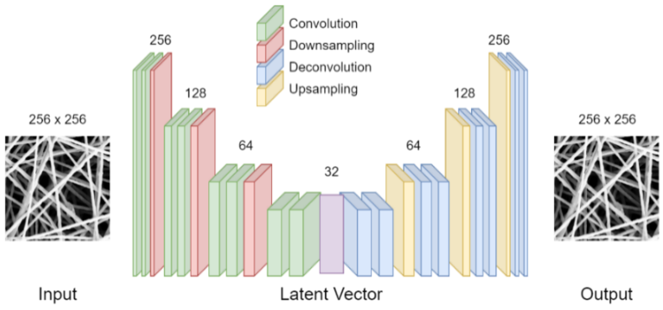
Figure 1.
Structure of Autoencoder.
Figure 1.
Structure of Autoencoder.
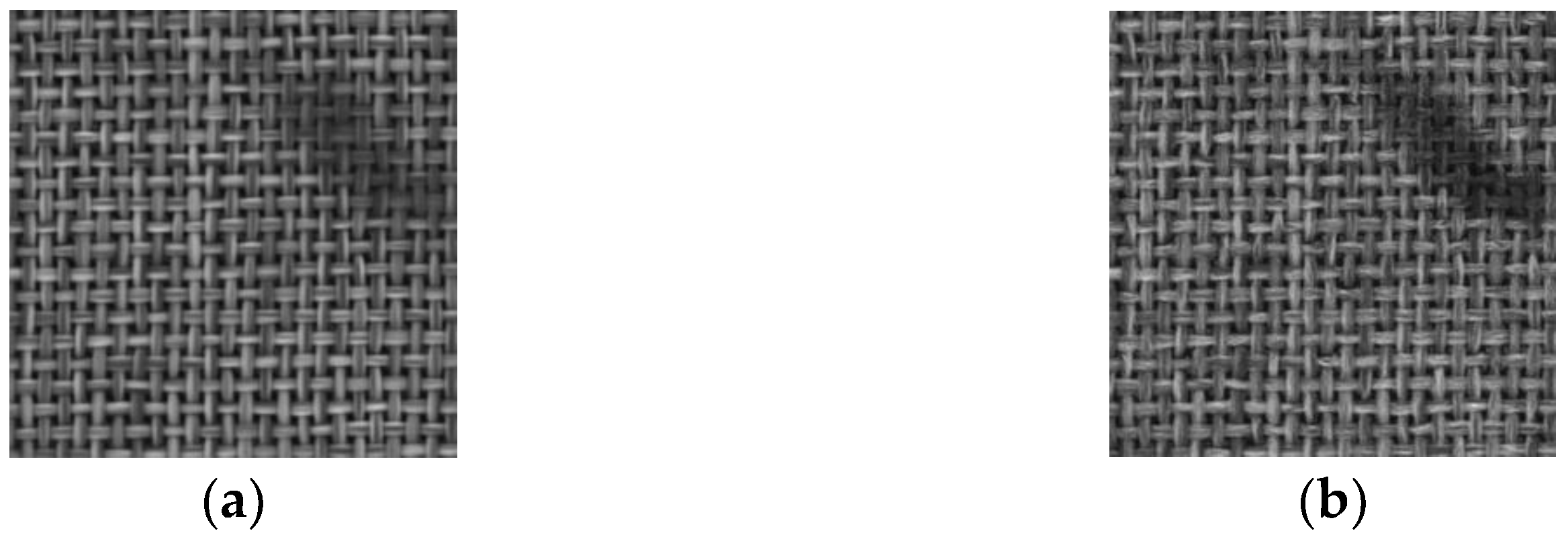
Figure 2.
(a) A test defect image. (b) Reconstructed image through general Autoencoder.
Figure 2.
(a) A test defect image. (b) Reconstructed image through general Autoencoder.
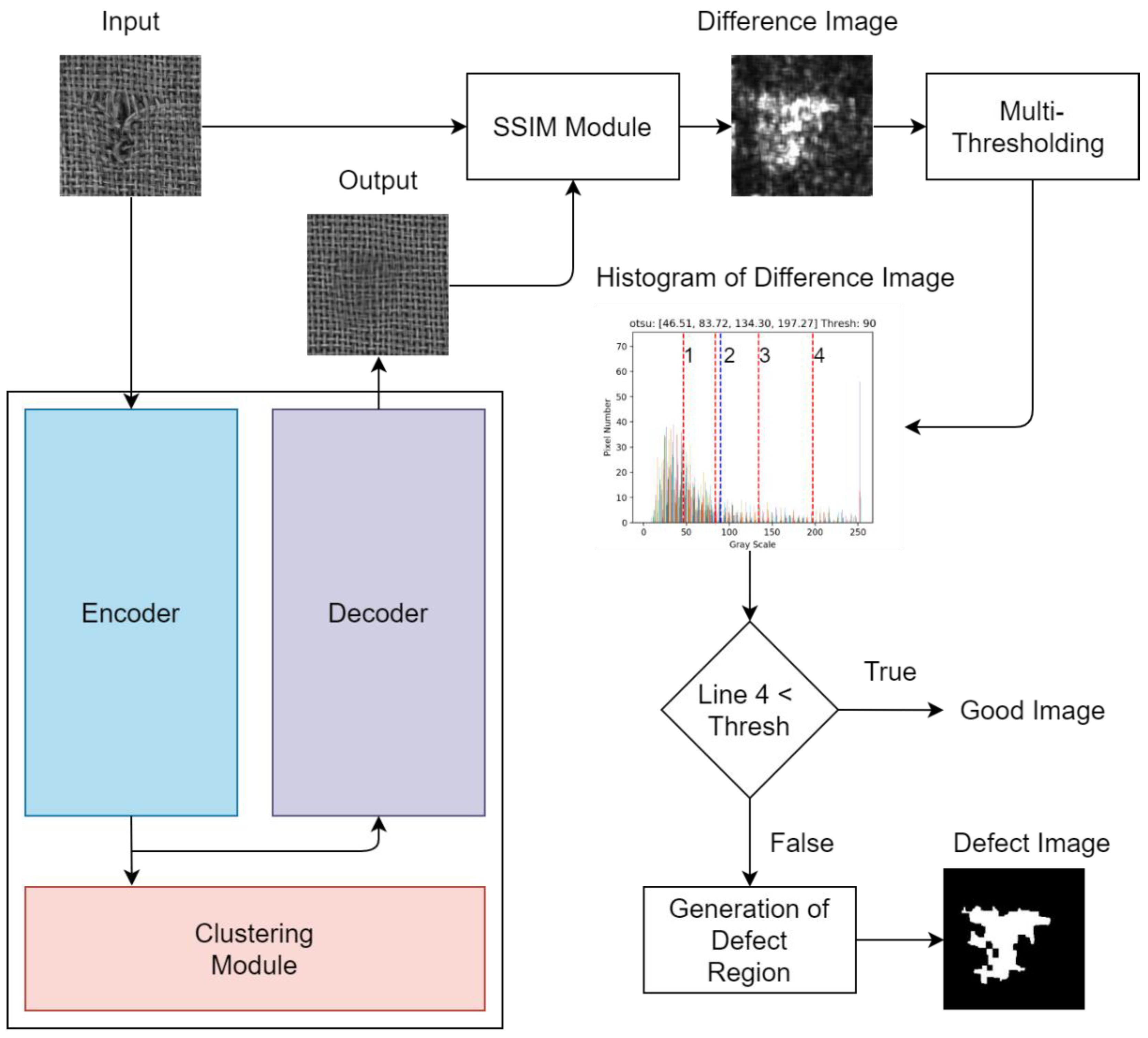
Figure 3.
Defect image detection architecture. The input defect image is reconstructed by the proposed Autoencoder, and the defect area is repaired with the correct texture pattern. The SSIM matching function is used to compute the difference between the input and output images, and then the multi-threshold image segmentation algorithm is used to classify the normal and defect images.
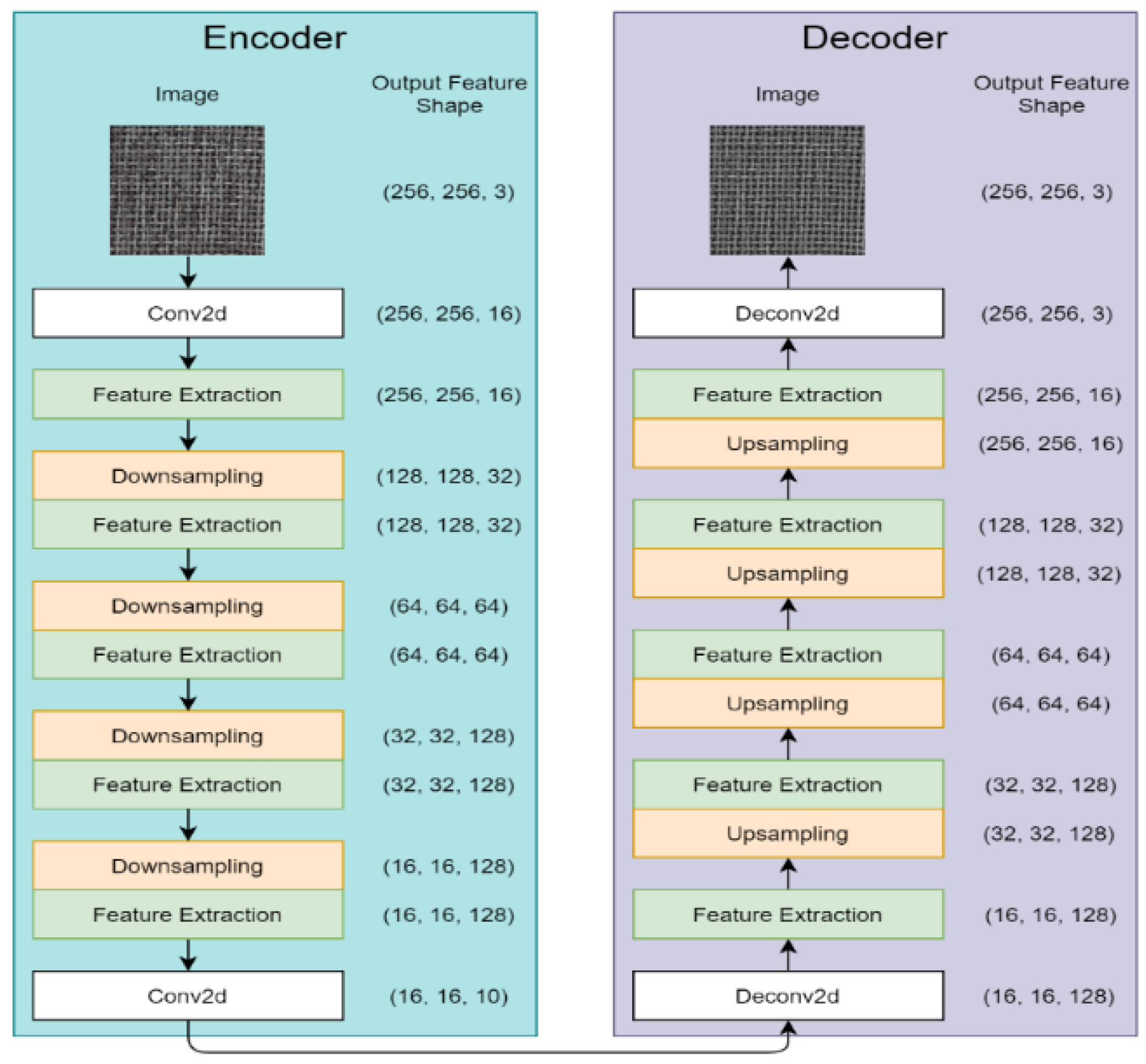
Figure 4.
Structure of the proposed Autoencoder model.
Figure 4.
Structure of the proposed Autoencoder model.
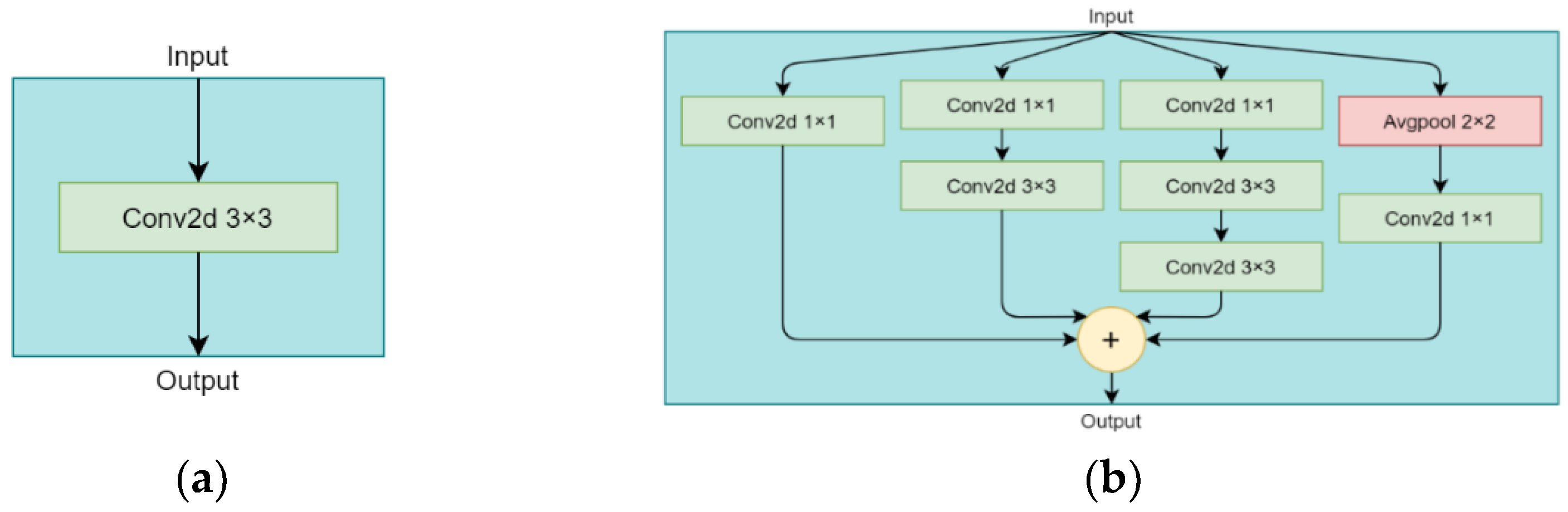
Figure 5.
(a) Simple convolution module. (b) Inception convolution module.
Figure 5.
(a) Simple convolution module. (b) Inception convolution module.
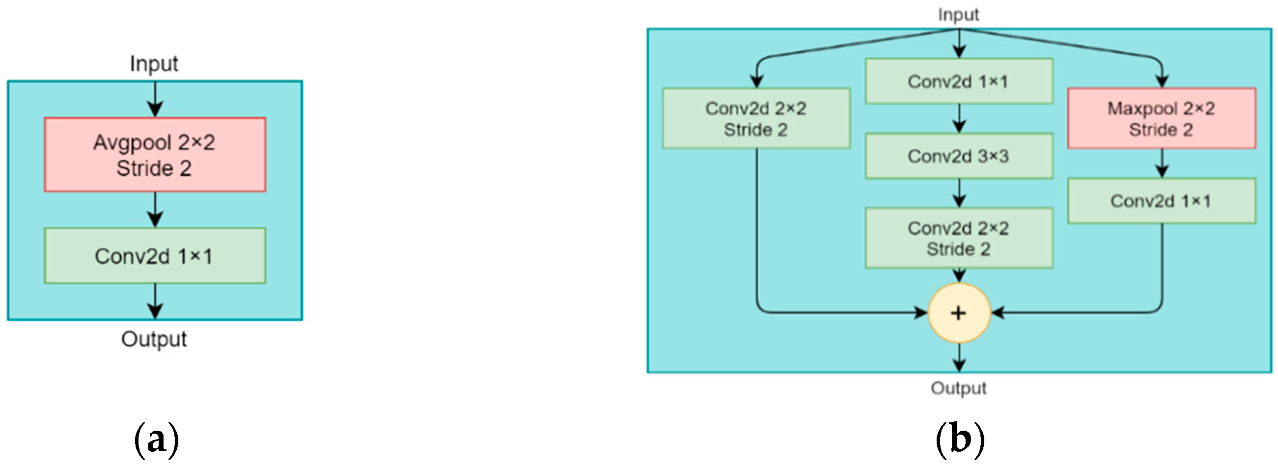
Figure 6.
(a) Simple downsampling module. (b) Inception downsampling module.
Figure 6.
(a) Simple downsampling module. (b) Inception downsampling module.
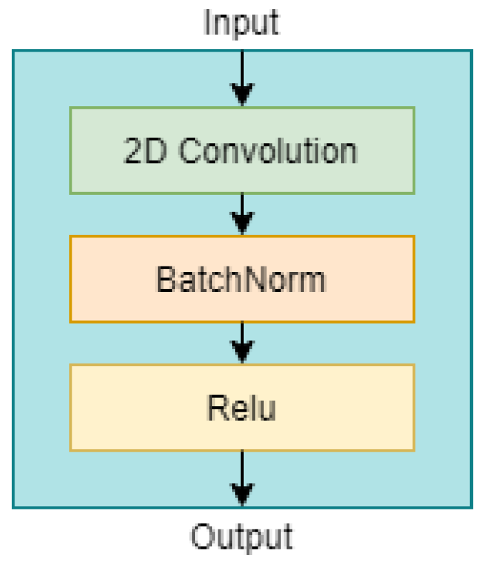
Figure 7.
Structure of Conv2d module.
Figure 7.
Structure of Conv2d module.
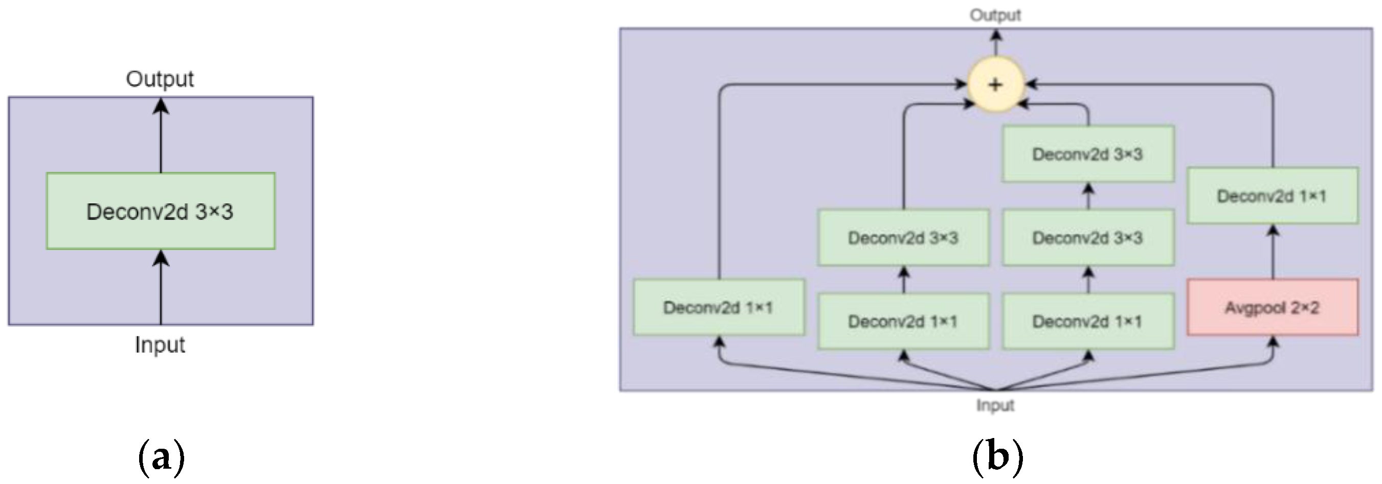
Figure 8.
(a) Simple deconvolution module. (b) Inception deconvolution module.
Figure 8.
(a) Simple deconvolution module. (b) Inception deconvolution module.
Figure 9.
(a) Simple upsampling module. (b) Inception upsampling module.
Figure 9.
(a) Simple upsampling module. (b) Inception upsampling module.
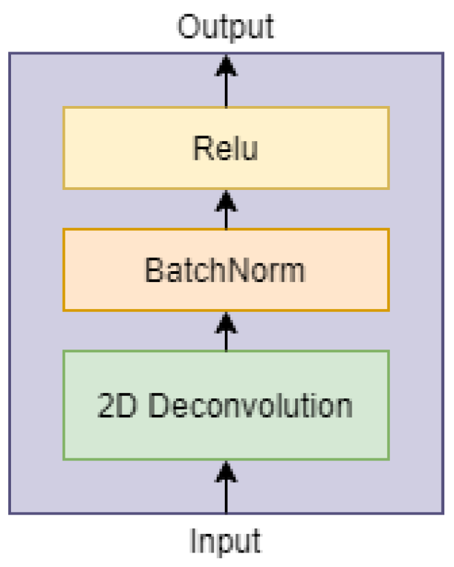
Figure 10.
Structure of Deconv2d module.
Figure 10.
Structure of Deconv2d module.
Figure 11.
The Autoencoder model with defect area repair capability.
Figure 11.
The Autoencoder model with defect area repair capability.
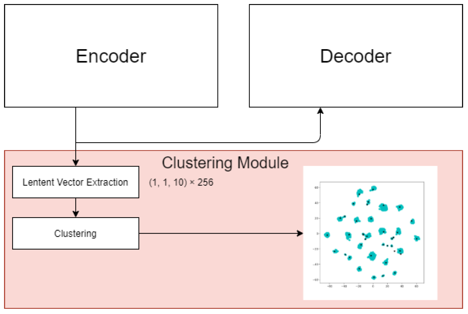
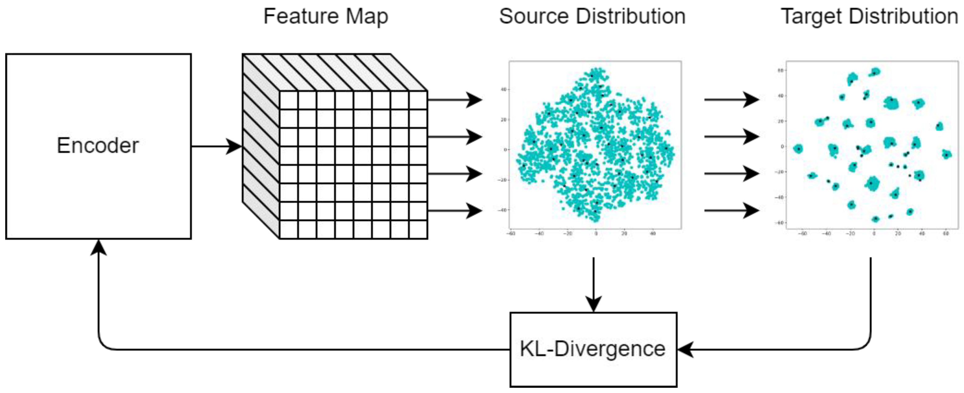
Figure 12.
The KL-Divergence function is used to modify the parameters of the encoder to cluster the latent vectors.
Figure 12.
The KL-Divergence function is used to modify the parameters of the encoder to cluster the latent vectors.
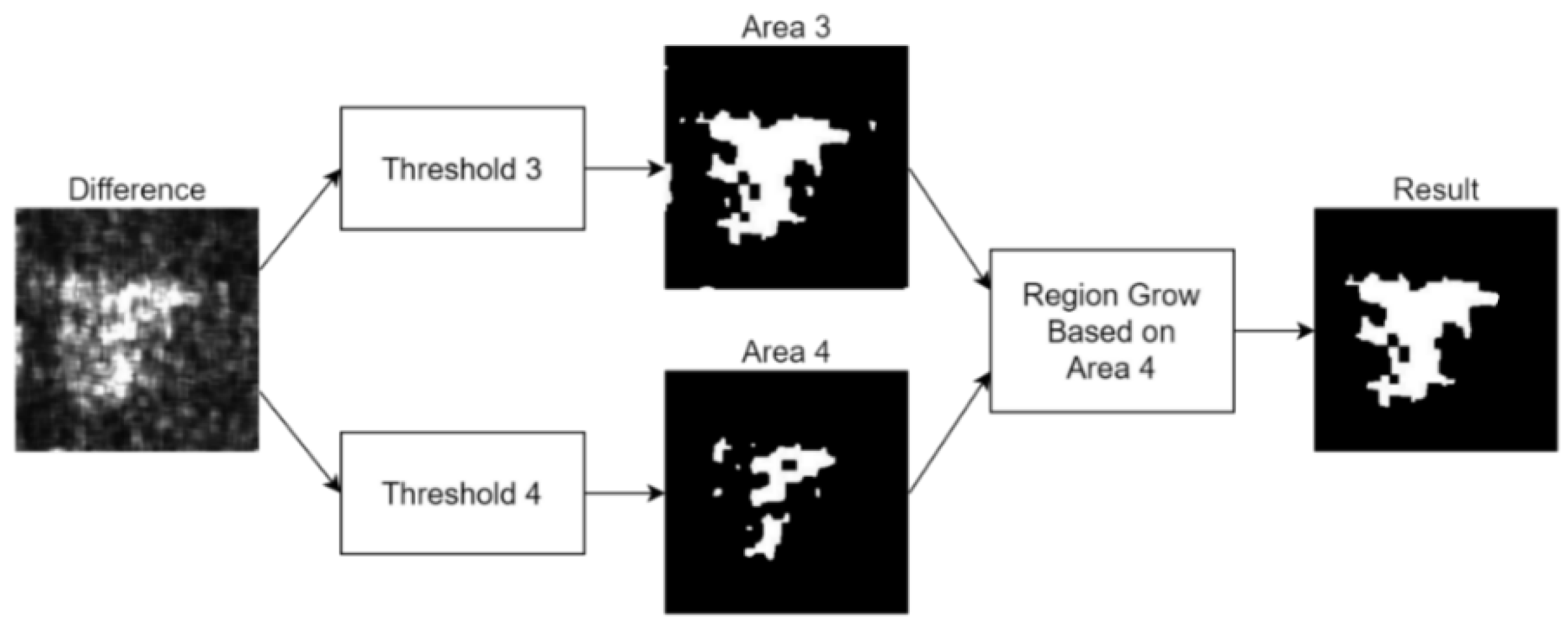
Figure 13.
If the input image is classified as a defect image, the third and fourth thresholds will be used to binarize the difference image to mark the defect area.
Figure 13.
If the input image is classified as a defect image, the third and fourth thresholds will be used to binarize the difference image to mark the defect area.
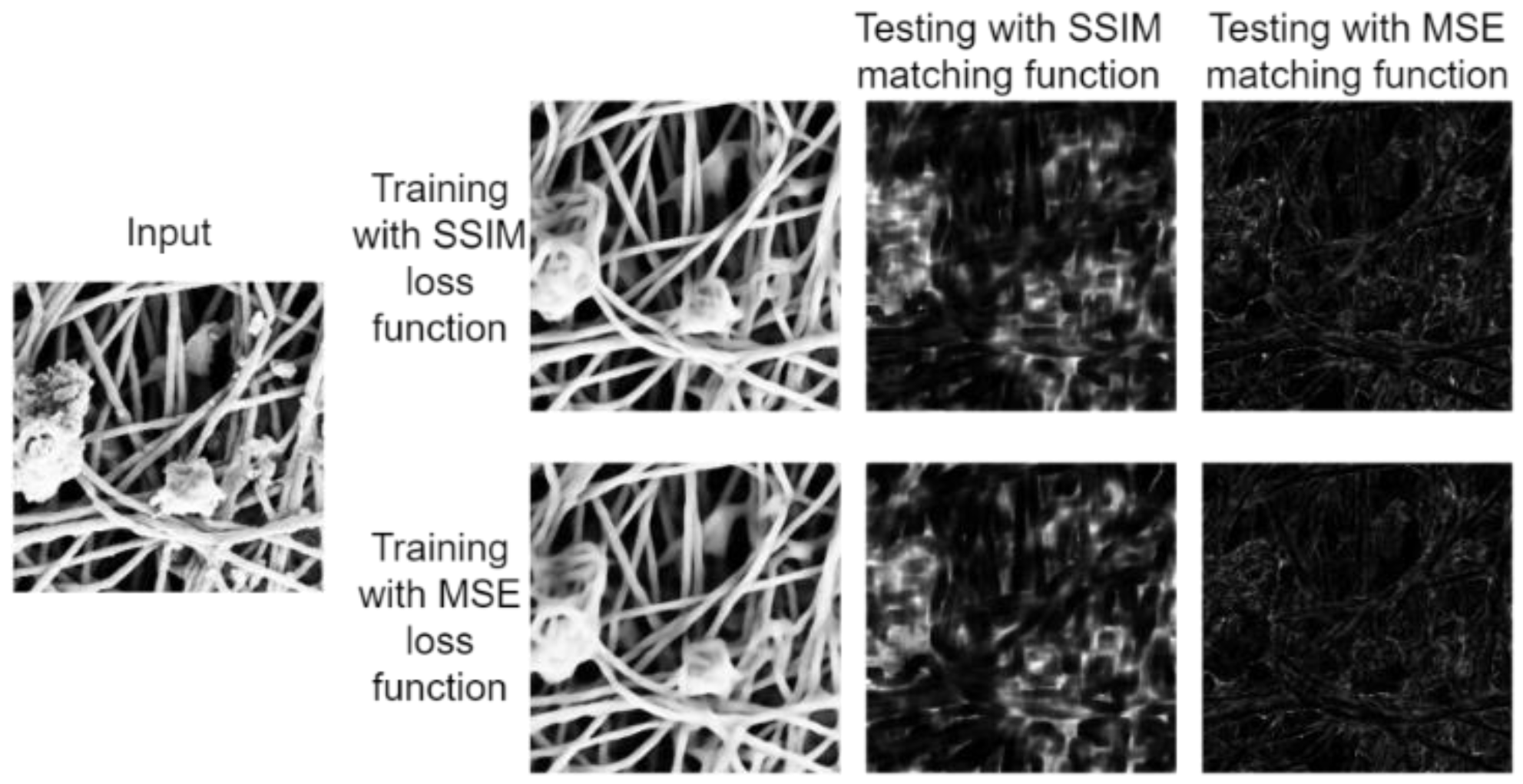
Figure 14.
The subjective evaluation of the reconstruction quality using SSIM and MSE as the training and testing functions on the normal nanofiber images.
Figure 14.
The subjective evaluation of the reconstruction quality using SSIM and MSE as the training and testing functions on the normal nanofiber images.
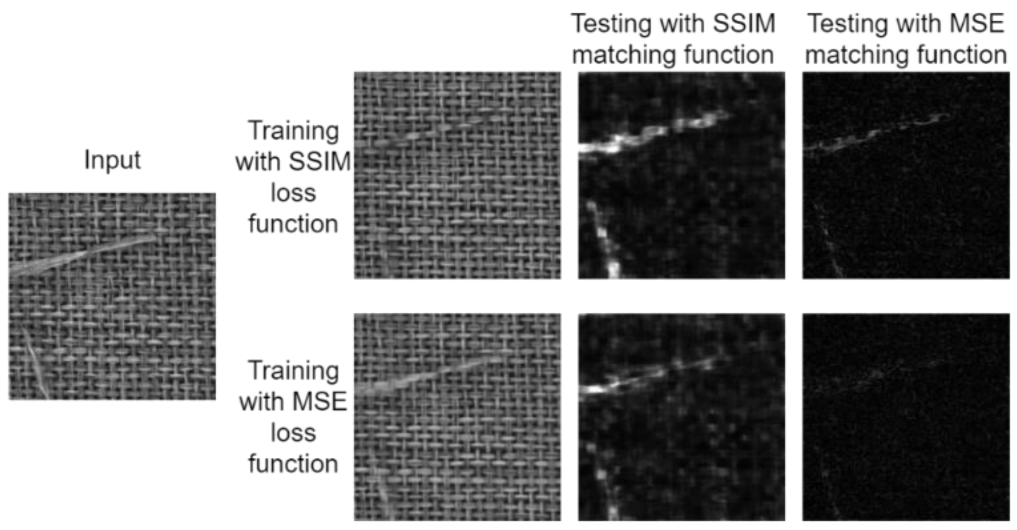
Figure 15.
The subjective evaluation of the reconstruction quality using SSIM and MSE as the training and testing functions on the normal carpet images.
Figure 15.
The subjective evaluation of the reconstruction quality using SSIM and MSE as the training and testing functions on the normal carpet images.
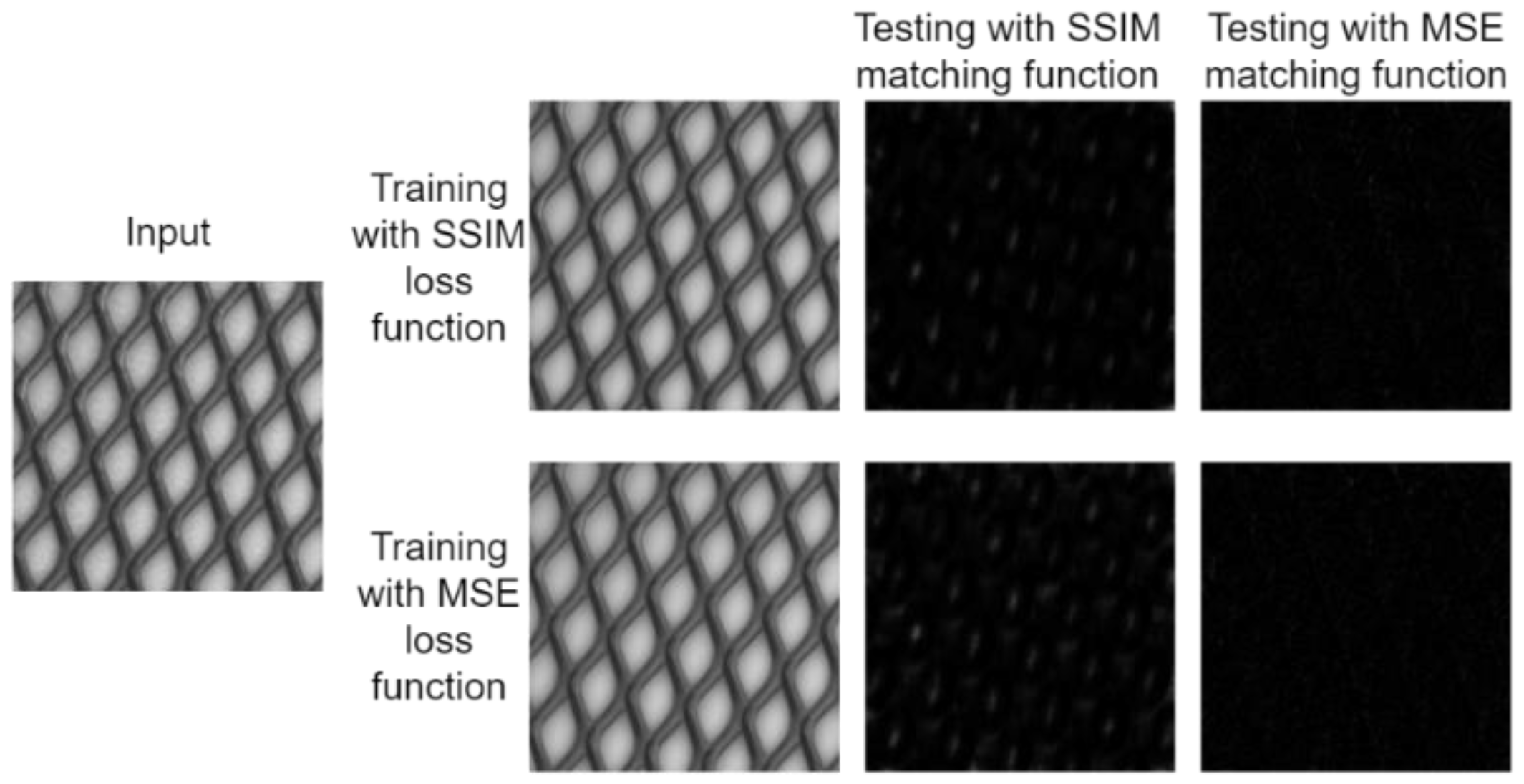
Figure 16.
The subjective evaluation of the reconstruction quality using SSIM and MSE as the training and testing functions on the normal grid images.
Figure 16.
The subjective evaluation of the reconstruction quality using SSIM and MSE as the training and testing functions on the normal grid images.
Figure 17.
The subjective evaluation of repair quality using SSIM and MSE as the training and testing functions on defective nanofiber images.
Figure 17.
The subjective evaluation of repair quality using SSIM and MSE as the training and testing functions on defective nanofiber images.
Figure 18.
The subjective evaluation of repair quality using SSIM and MSE as the training and testing functions on defective carpet images.
Figure 18.
The subjective evaluation of repair quality using SSIM and MSE as the training and testing functions on defective carpet images.
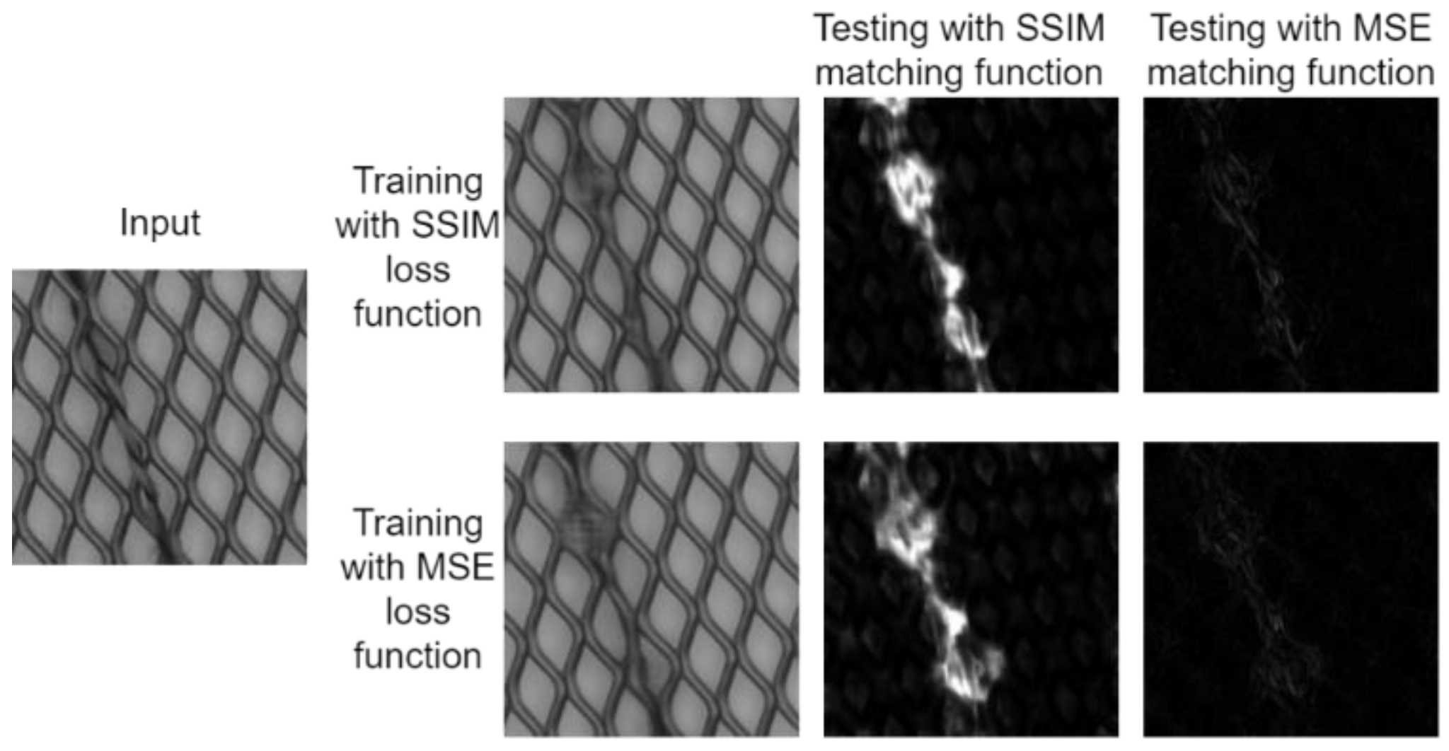
Figure 19.
The subjective evaluation of repair quality using SSIM and MSE as the training and testing functions on defective grid images.
Figure 19.
The subjective evaluation of repair quality using SSIM and MSE as the training and testing functions on defective grid images.
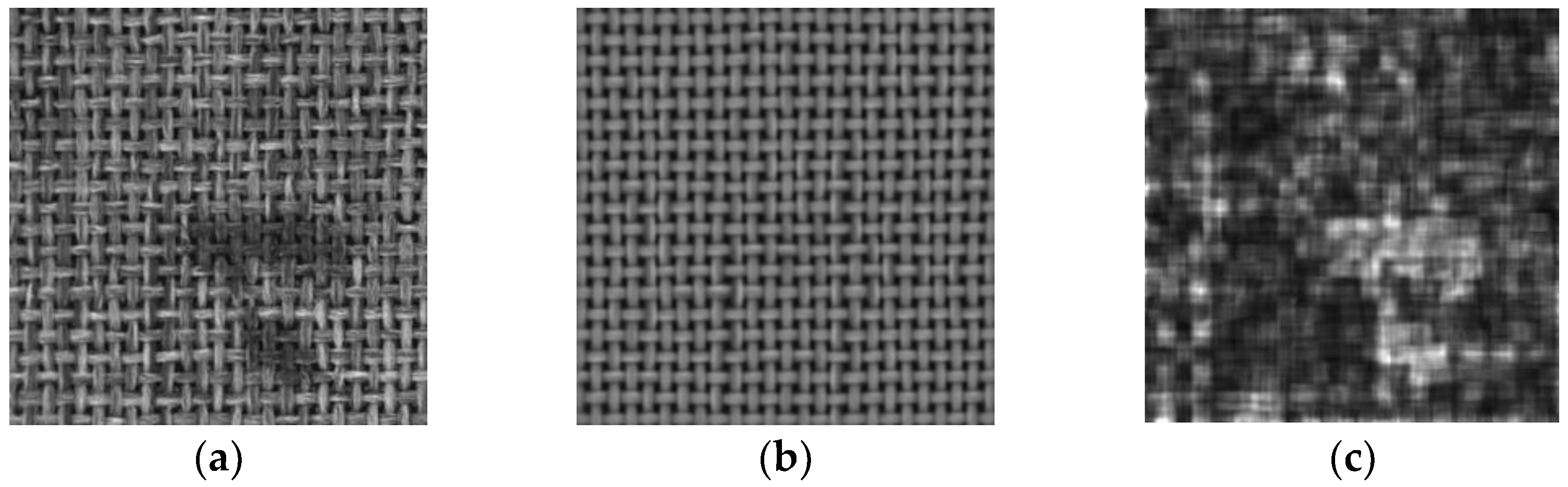
Figure 20.
Simulation result for higher weight of SSIM loss function. (a) The defective carpet image. (b) The reconstructed image for image (a). (c) The difference image between images (a,b) obtained by SSIM function.
Figure 20.
Simulation result for higher weight of SSIM loss function. (a) The defective carpet image. (b) The reconstructed image for image (a). (c) The difference image between images (a,b) obtained by SSIM function.
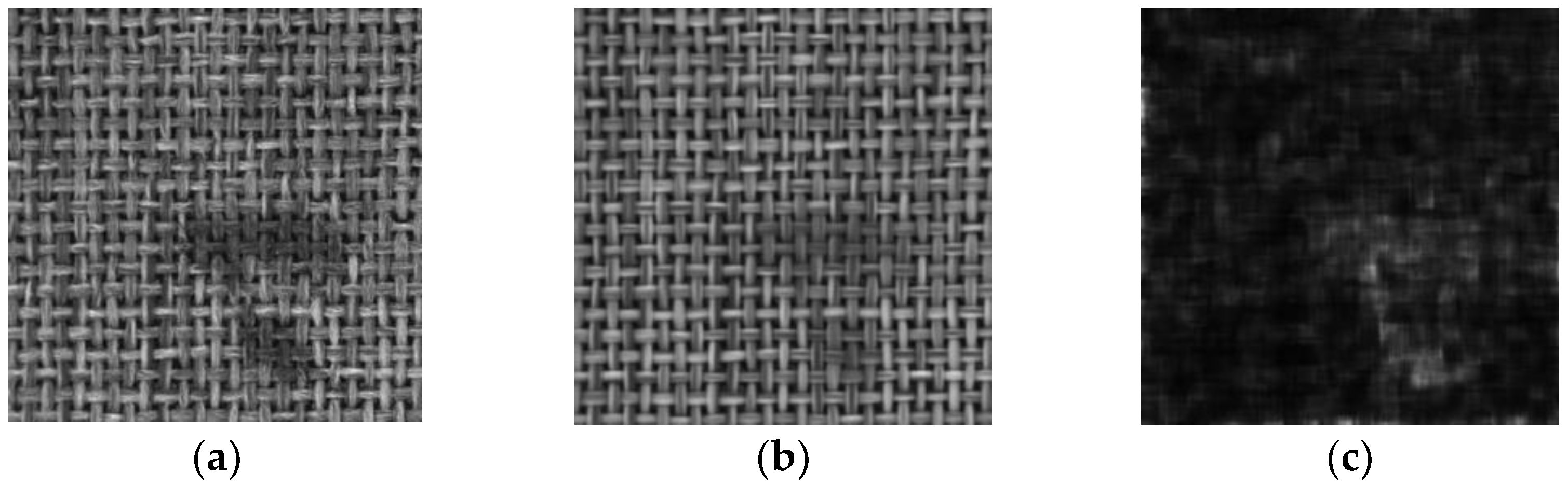
Figure 21.
Simulation result for higher weight of DEC loss function. (a) The defective carpet image. (b) The reconstructed image for image (a). (c) The difference image between images (a,b) obtained by SSIM function.
Figure 21.
Simulation result for higher weight of DEC loss function. (a) The defective carpet image. (b) The reconstructed image for image (a). (c) The difference image between images (a,b) obtained by SSIM function.
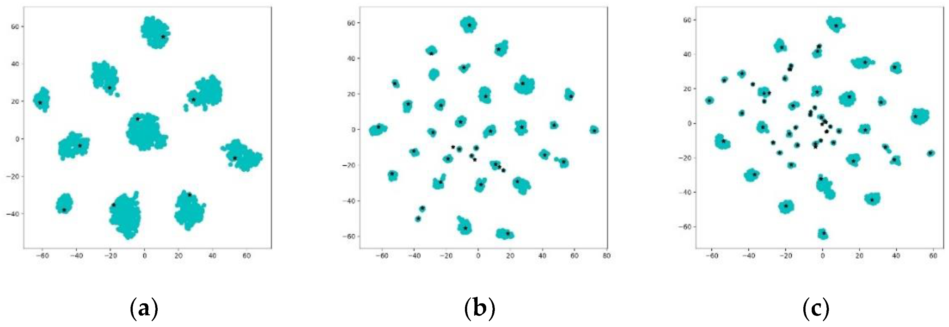
Figure 22.
The clustering analysis for different cluster number by using the latent vectors of carpet images. (a) k = 10. (b) k = 40. (c) k = 60.
Figure 22.
The clustering analysis for different cluster number by using the latent vectors of carpet images. (a) k = 10. (b) k = 40. (c) k = 60.
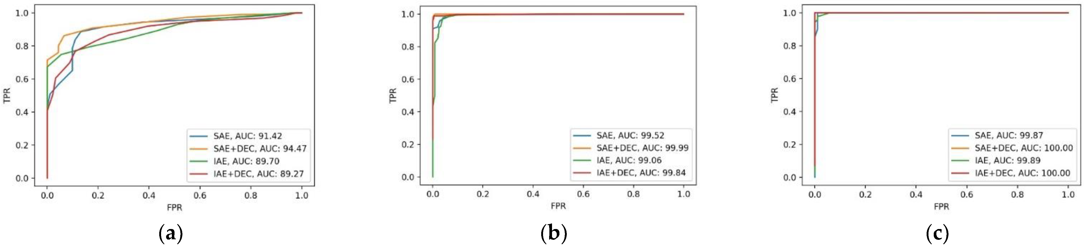
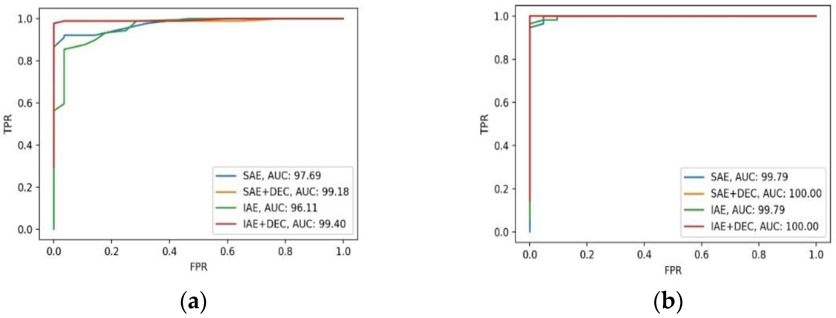
Figure 23.
The ROC curves of patch image simulation for (a) nanofiber, (b) carpet, and (c) grid datasets.
Figure 23.
The ROC curves of patch image simulation for (a) nanofiber, (b) carpet, and (c) grid datasets.
Figure 24.
The ROC curves of complete image simulation for (a) carpet and (b) grid datasets.
Figure 24.
The ROC curves of complete image simulation for (a) carpet and (b) grid datasets.
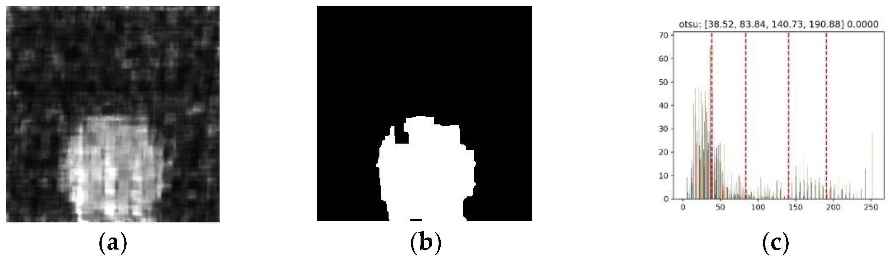
Figure 25.
Analysis of using multi-thresholding to identify the obvious defect carpet image. (a) Obvious difference image. (b) Apply Otsu multi-thresholding method to detect the defective area. (c) The result of multi-thresholding.
Figure 25.
Analysis of using multi-thresholding to identify the obvious defect carpet image. (a) Obvious difference image. (b) Apply Otsu multi-thresholding method to detect the defective area. (c) The result of multi-thresholding.
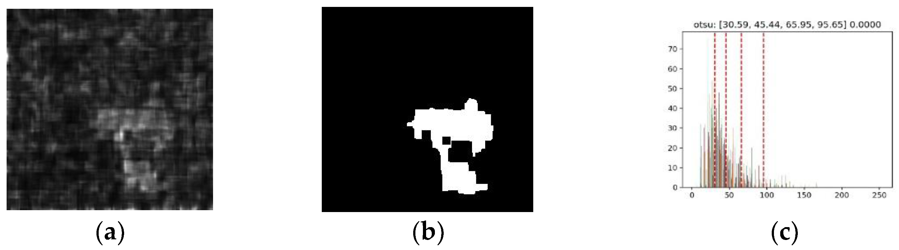
Figure 26.
Analysis of using multi-thresholding to identify the weak defect carpet image. (a) Weak difference image. (b) Apply Otsu multi-thresholding method to detect the defective area. (c) The result of multi-thresholding.
Figure 26.
Analysis of using multi-thresholding to identify the weak defect carpet image. (a) Weak difference image. (b) Apply Otsu multi-thresholding method to detect the defective area. (c) The result of multi-thresholding.
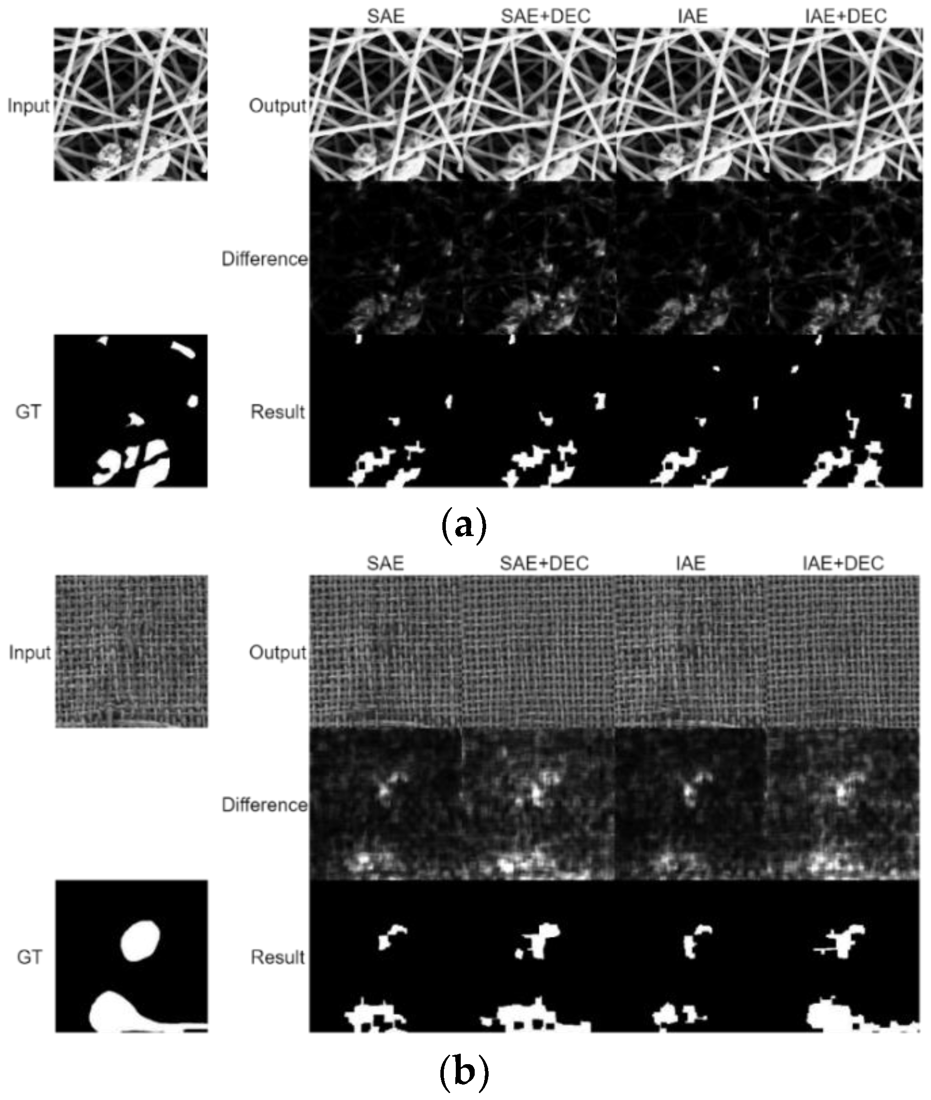
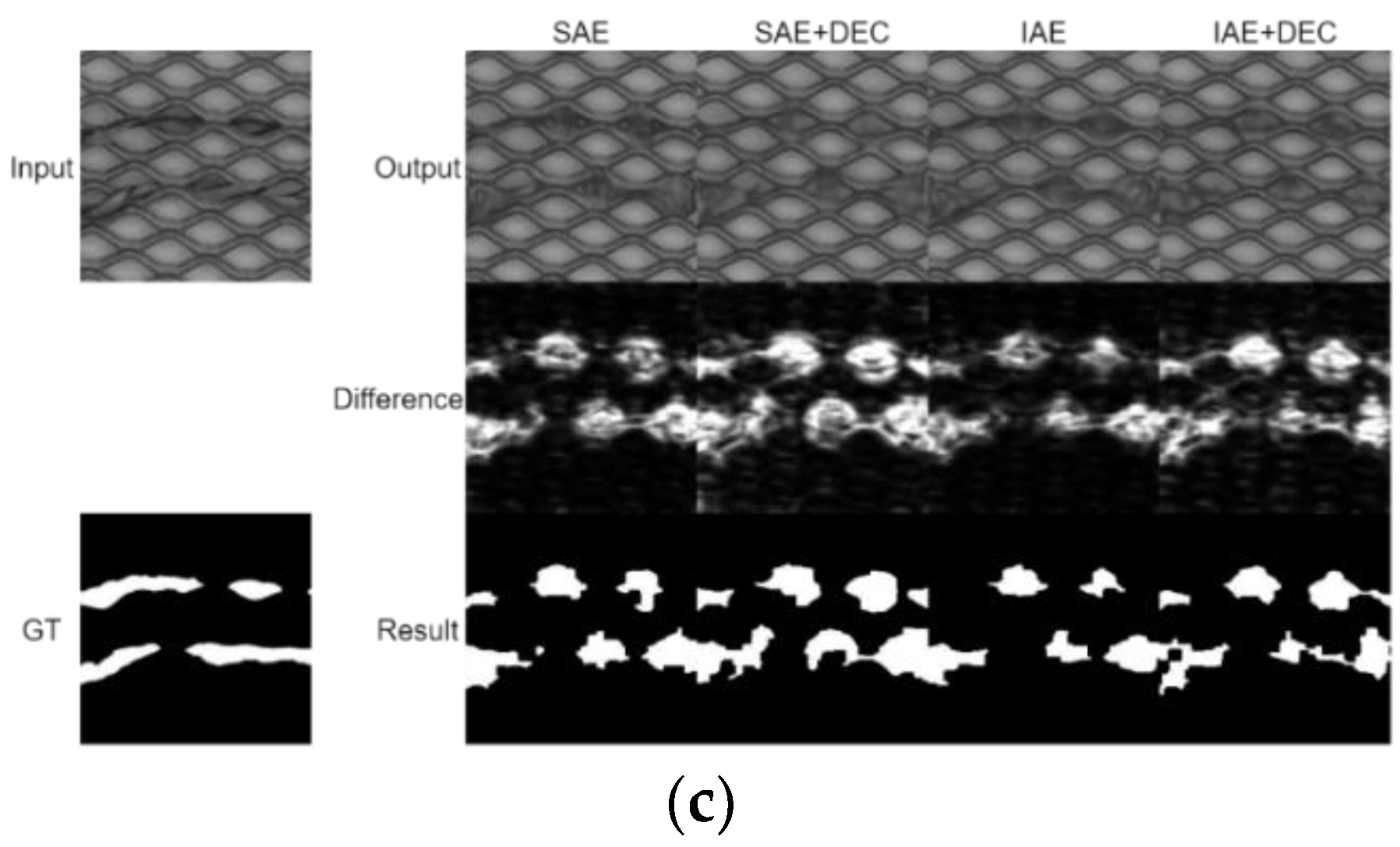
Figure 27.
The defect detection results of the four models on (a) nanofiber, (b) carpet, and (c) grid datasets for the subjective evaluation.
Figure 27.
The defect detection results of the four models on (a) nanofiber, (b) carpet, and (c) grid datasets for the subjective evaluation.
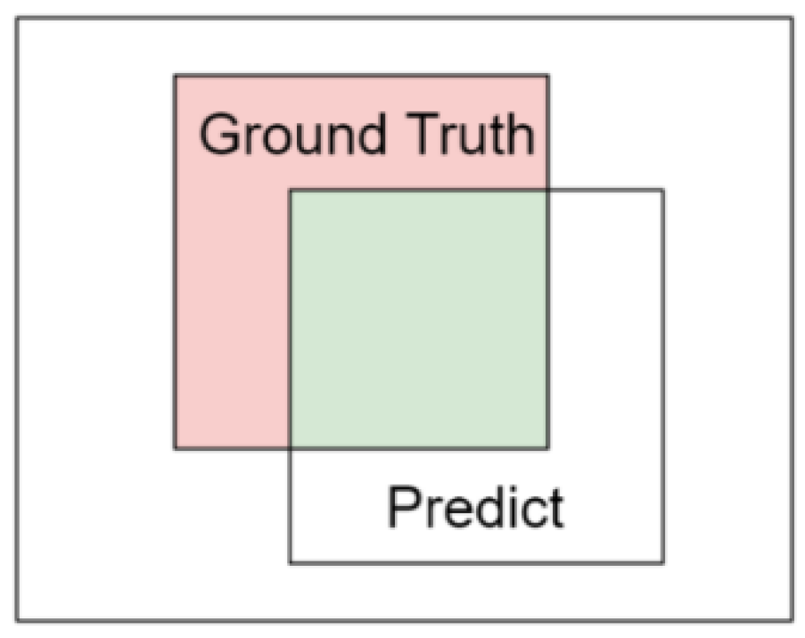
Figure 28.
The method of analyzing the accuracy of detected defective area.
Figure 28.
The method of analyzing the accuracy of detected defective area.
Table 1.
Dataset of nanofiber image.
Table 1.
Dataset of nanofiber image.
| | Training Data | Testing Data |
|---|
| Category | Good | Good | Defect |
| Amount (frame) | 4 | 1 | 40 |
| Image size | 1024 × 700 | 1024 × 700 | 1024 × 696 |
Table 2.
Dataset of carpet image.
Table 2.
Dataset of carpet image.
| | Training Data | Testing Data |
|---|
| Category | Good | Good | Color | Cut | Hole | Metal | Thread |
| Amount (frame) | 277 | 28 | 19 | 17 | 17 | 17 | 19 |
| Image size | 1024 × 1024 |
Table 3.
Dataset of grid image.
Table 3.
Dataset of grid image.
| | Training Data | Testing Data |
|---|
| Category | Good | Good | Bent | Broken | Glue | Metal | Thread |
| Amount (frame) | 264 | 21 | 12 | 12 | 11 | 11 | 11 |
| Image size | 1024 × 1024 |
Table 4.
Analysis of reconstruction error using Simple Autoencoder for normal image.
Table 4.
Analysis of reconstruction error using Simple Autoencoder for normal image.
| | Nanofiber | Carpet | Grid |
|---|
| | Testing with SSIM Matching Function | Testing with MSE Matching Function | Testing with SSIM Matching Function | Testing with MSE Matching Function | Testing with SSIM Matching Function | Testing with MSE Matching Function |
|---|
| Training with SSIM loss function | 0.1440 | 479.05 | 0.1171 | 202.09 | 0.0361 | 21.50 |
| Training with MSE loss function | 0.1739 | 458.81 | 0.1386 | 177.62 | 0.0554 | 29.77 |
Table 5.
Analysis of reconstruction error using Inception Autoencoder for normal image.
Table 5.
Analysis of reconstruction error using Inception Autoencoder for normal image.
| | Nanofiber | Carpet | Grid |
|---|
| | Testing with SSIM Matching Function | Testing with MSE Matching Function | Testing with SSIM Matching Function | Testing with MSE Matching Function | Testing with SSIM Matching Function | Testing with MSE Matching Function |
|---|
| Training with SSIM loss function | 0.1287 | 403.63 | 0.1055 | 178.77 | 0.0322 | 19.92 |
| Training with MSE loss function | 0.1400 | 348.88 | 0.1277 | 168.04 | 0.0455 | 23.70 |
Table 6.
Weighting ratios between SSIM and DEC loss functions for Simple and Inception Autoencoders.
Table 6.
Weighting ratios between SSIM and DEC loss functions for Simple and Inception Autoencoders.
| | Nanofiber | Carpet | Grid |
|---|
| Model | SSIM:DEC |
| Simple AE | 300:1 | 140:1 | 80:1 |
| Inception AE | 110:1 | 80:1 | 100:1 |
Table 7.
Classification thresholds for three datasets.
Table 7.
Classification thresholds for three datasets.
| | Nanofiber | Carpet | Grid |
|---|
| Threshold | 90 | 90 | 80 |
Table 8.
Accuracy analysis of classifying normal and defect patch nanofiber images.
Table 8.
Accuracy analysis of classifying normal and defect patch nanofiber images.
| Model | Good | Defect |
|---|
| SAE | 90.10% | 65.13% |
| SAE + DEC | 82.41% | 90.79% |
| IAE | 100% | 67.31% |
| IAE + DEC | 75.82% | 86.68% |
Table 9.
Accuracy analysis of classifying normal and defect patch carpet images.
Table 9.
Accuracy analysis of classifying normal and defect patch carpet images.
| Model | Good | Color | Cut | Hole | Metal | Thread |
|---|
| SAE | 100% | 40.57% | 92.50% | 90.14% | 93.54% | 90.69% |
| SAE + DEC | 99.19% | 100% | 100% | 100% | 100% | 100% |
| IAE | 99.19% | 21.73% | 88.75% | 83.09% | 91.93% | 79.06% |
| IAE + DEC | 99.59% | 91.30% | 100% | 98.59% | 100% | 98.83% |
Table 10.
Accuracy analysis of classifying normal and defect patch grid images.
Table 10.
Accuracy analysis of classifying normal and defect patch grid images.
| Model | Good | Bent | Broken | Glue | Metal | Thread |
|---|
| SAE | 98.94% | 88.23% | 93.75% | 82.75% | 100% | 98.57% |
| SAE + DEC | 100% | 100% | 100% | 100% | 100% | 100% |
| IAE | 100% | 85.29% | 81.25% | 58.62% | 94.28% | 91.42% |
| IAE + DEC | 100% | 100% | 100% | 96.55% | 94.28% | 100% |
Table 11.
Classification accuracy for complete nanofiber images.
Table 11.
Classification accuracy for complete nanofiber images.
| | Nanofiber |
|---|
| | Good | Defect |
|---|
| SAE | - | 95% |
| SAE + DEC | - | 100% |
| IAE | - | 100% |
| IAE + DEC | - | 100% |
Table 12.
Classification accuracy for complete carpet images.
Table 12.
Classification accuracy for complete carpet images.
| | Carpet |
|---|
| | Good | Color | Cut | Hole | Metal | Thread |
|---|
| SAE | 100% | 42.10% | 100% | 94.11% | 100% | 89.47% |
| SAE + DEC | 89.29% | 94.73% | 100% | 100% | 100% | 100% |
| IAE | 96.50% | 42.10% | 100% | 100% | 100% | 78.94% |
| IAE + DEC | 96.50% | 94.73% | 100% | 100% | 100% | 100% |
Table 13.
Classification accuracy for complete grid images.
Table 13.
Classification accuracy for complete grid images.
| | Grid |
|---|
| | Good | Bent | Broken | Glue | Metal | Thread |
|---|
| SAE | 95.30% | 100% | 100% | 90.90% | 100% | 100% |
| SAE + DEC | 100% | 100% | 100% | 100% | 100% | 100% |
| IAE | 100% | 100% | 100% | 72.72% | 100% | 100% |
| IAE + DEC | 100% | 100% | 100% | 90.90% | 100% | 100% |
Table 14.
Comparison of the four proposed models with the models in [
14].
Table 14.
Comparison of the four proposed models with the models in [
14].
| | Carpet | Grid |
|---|
| Model | Good | Defect | Good | Defect |
|---|
| SAE | 100% | 85% | 95% | 98% |
| SAE + DEC | 89% | 98% | 100% | 100% |
| IAE | 96% | 84% | 100% | 94% |
| IAE + DEC | 96% | 98% | 100% | 98% |
| AE(SSIM) [14] | 43% | 90% | 38% | 100% |
| AE(L2) [14] | 57% | 42% | 57% | 98% |
| AnoGAN [14] | 82% | 16% | 90% | 12% |
| CNN Dict [14] | 89% | 36% | 57% | 33% |
Table 15.
Analysis of the accuracy of detected defective area with the methods in [
14].
Table 15.
Analysis of the accuracy of detected defective area with the methods in [
14].
| Models | Carpet | Grid |
|---|
| SAE | 56% | 58% |
| SAE + DEC | 76% | 74% |
| IAE | 48% | 53% |
| IAE + DEC | 78% | 73% |
| AE(SSIM) [14] | 69% | 88% |
| AE(L2) [14] | 38% | 83% |
| AnoGAN [14] | 34% | 4% |
| CNN Dict [14] | 20% | 2% |


