Article

Design of Two-Mode Spectroscopic Sensor for Biomedical Applications: Analysis and Measurement of Relative Intensity Noise through Control Mechanism

1
Faculty of Electrical and Electronics Engineering, University of Engineering and Technology, Taxila 47050, Pakistan
2
Faculty of Electrical Engineering and Computer Science, University of Kassel, 34125 Kassel, Germany
3
Faculty of Engineering and Computer Science, National University of Modern Languages, Islamabad 44000, Pakistan
4
Department of Mechanical and Aerospace Engineering, Sapienza University of Rome, 00184 Rome, Italy
5
Faculty of Engineering and Applied Sciences, Riphah International University, Islamabad 44000, Pakistan
6
Department of Maths and Stats, International Islamic University, Islamabad 44000, Pakistan
7
Faculty of Information & Communication Technology, Balochistan University of Information Technology, Engineering and Management Sciences, Quetta 87300, Pakistan
8
Faculty of Engineering, Bahria University, Lahore Campus, 47-C Civic Center Johar Town, Lahore 54000, Pakistan
9
Department of Computer Sciences, Bahria University, Lahore Campus, 47-C Civic Center Johar Town, Lahore 54000, Pakistan
10
Department of Mechanical Engineering, College of EME, National University of Science and Technology, Peshawar Road, Rawalpindi 46000, Pakistan
11
Department of Mechanical Engineering, Institute of Space Technology, Islamabad 44000, Pakistan
*
Authors to whom correspondence should be addressed.
Appl. Sci. 2022, 12(4), 1856; https://doi.org/10.3390/app12041856
Submission received: 9 September 2021 / Revised: 20 December 2021 / Accepted: 14 January 2022 / Published: 11 February 2022
(This article belongs to the Special Issue Frontiers in Optical Materials)

Abstract

:
The design of an intracavity spectroscopy based two-mode biomedical sensor involves a thorough investigation of the system. For this purpose, the individual components that are present in the system must be examined. This work describes the principle of two very important gadgets, namely the Fibre Bragg Grating (FBG), and the tunable coupler. We adhere to a Petri network scheme to model and analyze the performance of the FBG, and the results mirror strikingly low difference in the values of Bragg Wavelength during its ascending and descending operational principle, thereby maintaining the accuracy of the sensor’s results. Next, a pseudocode is developed and implemented for the investigation of the optical coupler in LabView. The values of its maximum output power are determined, and the coupling ratio for various values of controlling voltage is determined at three different wavelengths. The hysteresis results mirror an extremely low difference between the forward and reverse values in the results. Both the results of the FBG and the coupler are thereby extremely reliable to use them in the laser system, as evident from the respective intensity noise outcomes, as well as the experimentation on substances of interest (Dichloro Methane and Propofol).

1. Introduction

Considering the living conditions at present occasions, various procedures are being created and explored to check these illnesses [1,2,3]. Since the pivotal centre of attention is human life, the inquest stays focused on different aspects [4,5,6,7]. One of them is the air that is being breathed out of the human lungs. Using the information from this air, data in regards to various sicknesses can be found out. An important tool in this connection that can be utilized is spectroscopy, which helps in the examination of a specific material, potentially recognized as Volatile Organic Compounds (VOCs) nicknamed biomarkers) [8,9,10,11]. This in turn guides us to critical analysis regarding research in environmental and organic disciplines [5,12,13,14], with substantially tremendous capacity in the future.
The current research originates from the hypothesis of intracavity absorption spectroscopy in which a material is put within the cavity of the laser [15,16,17]. The rudimentary difference between this method and the conventional intercavity absorption spectroscopy is that the latter method investigates the material of interest when it is placed outside the laser cavity [7,18]. However, the former technique is based on placing the substance of interest inside the laser cavity [19]. On account of this fact, investigation hereby reveals that this technique is extremely susceptible even to little changes in the material [20,21], in contrast with intercavity spectroscopy, as said material is put within the cavity. This phenomenon can be used to understand minute variations in said substance, after being placed inside the laser cavity [22,23]. This is a very tempting behaviour which can be extrapolated in a biomedical sensor. As a result, the technique of intracavity absorption spectroscopy throngs attention from the investigators [24,25]. Therefore, this is the foundation of our laser based system. It has been recently reported that multiple modes can be confined in a nanocavity using metamaterials, and the strength of their electric field is very high [26,27,28], which motivates us to use more than one modes inside our proposed sensor setup. Our endeavour is to utilize two modes (frequencies) which makes the measurements more sensitive. Initially, the utilization of single mode does not provide effective outcomes. Thus, a dual mode framework provides more sensitive and accurate results. Afterwards, utilizing many modes is prone to increase the price and complexity of the anticipated biomedical application, which should not be helpful for the pragmatic viewpoint. Based on these arguments, this work attempts to utilize a dual mode framework, which is the first of its kind until now [15,29,30].
The principle of Fibre Bragg Gratings (FBGs) and controlling their wavelengths have been continuously used in the past for various applications in sensors [31,32]. The efficiency of a setup with FBGs can be improved by governing the devices with the aid of an automated mechanism which is helpful in saving much time and effort [33]. During the design of long gratings, selected etching techniques can be combined with fibre cladding to precise the amount of light which is being emitted from their respective wavelengths [34]. This work at the miniaturized level has been done since the aberration techniques became technically feasible [35], and was enhanced to high resolution images to explore samples in the laboratories [36]. Recent advancement in FBGs extends their applications to holograms that are currently being manufactured, tested and characterized in various forms [37]. On account of these techniques, the FBGs have been extensively used to detect various physical, chemical and biological parameters that might not be possible otherwise, without supplemental gadgets, which is supposedly not desirable for any sensors in the current world [32], in particular the health industry [38].

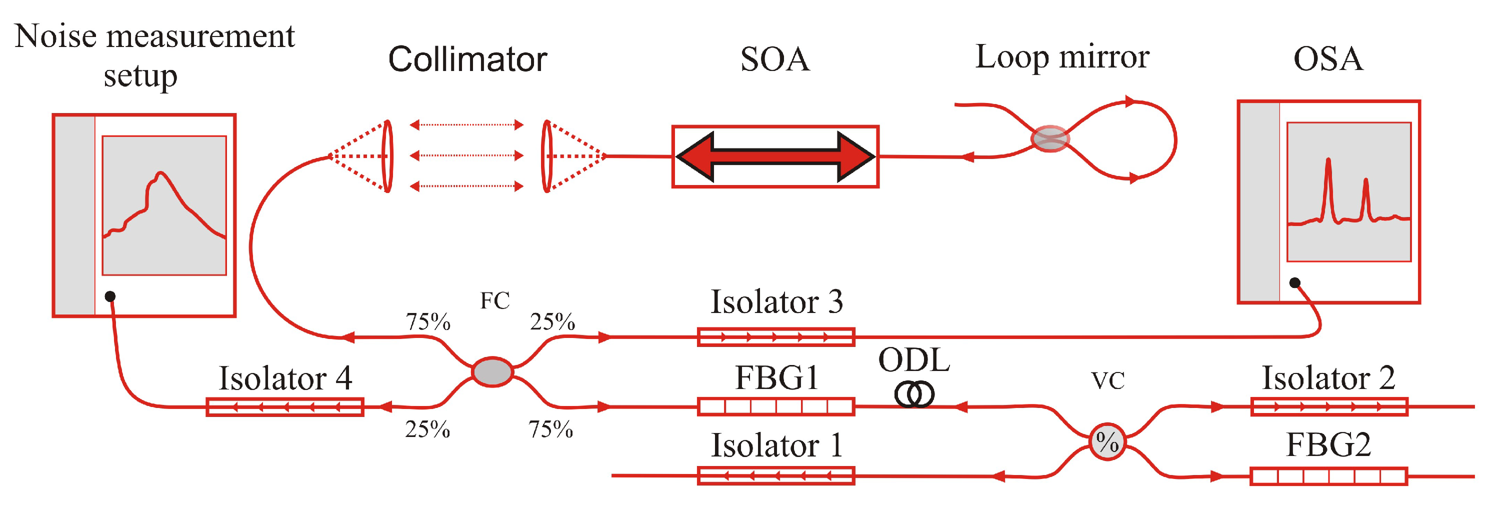
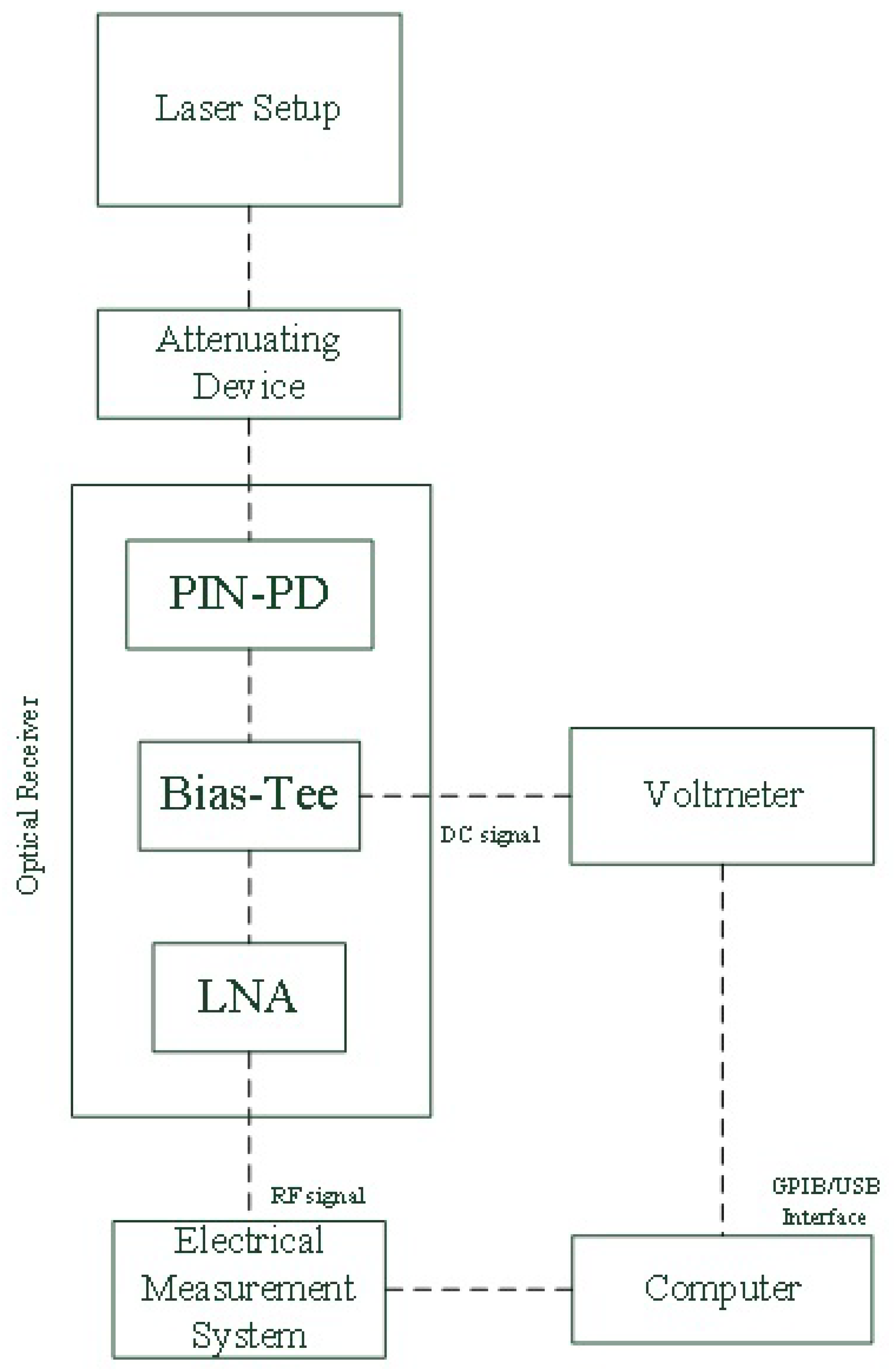
2. Experimental Setup

The laboratory system for this work has been elaborated in Figure 1 and Figure 2. This contains a Semiconductor Optical Amplifier (SOA), from which light is emitted in both directions in the Near Infra Red (NIR) range (1541–1545 nm). To intensify its output, the principle of optical reflection [17,39] has been created with the aid of loop mirror on one side. Thus, the output is provided into two Fiber Bragg Gratings, namely FBGi (FBGl/FBG1) and FBGo (FBGh/FBG2). These are in reference to the inner (lower wavelength) and outer (higher wavelength) cavities, respectively. These are separated with the help of optical couplers, VCi and VCo, which distinguish the two wavelengths (modes) Mi and Mo, respectively.
The SOA is supplied with injection current from the Laser Diode Controller (LDC), which also controls the temperature [40,41]. The collimator is the sample holder where the substance of interest can be placed. Isolators ensure unidirectional flow of optical light, for instance into the Optical Spectrum Analyzer (OSA), for the sake of measurement purpose [10,42,43,44].
The photodiode collects the light from the laser diode sensor. The electrical signal output from the photodiode contains DC signal as well as AC signal. To prevent saturation of the RF amplifier, the DC signal is filtered by using high frequency bandwidth Bias Tee. The DC signal from Bias Tee is measured using Digital Multimeter (DMM) and is equal to the average photocurrent I p , which is proportional to the mean optical intensity. The AC, which is proportional to the intensity noise of the laser, is amplified by Low Noise Amplifier (LNA). It is displayed and measured using radio frequency Electrical Spectrum Analyzer (ESA), whose attenuator can be set at 0 dB for high sensitivity measurement. The ESA [45] has a minimum resolution bandwidth of 10 Hz and typical noise figure of 21 dB @ 3 MHz resolution bandwidth.

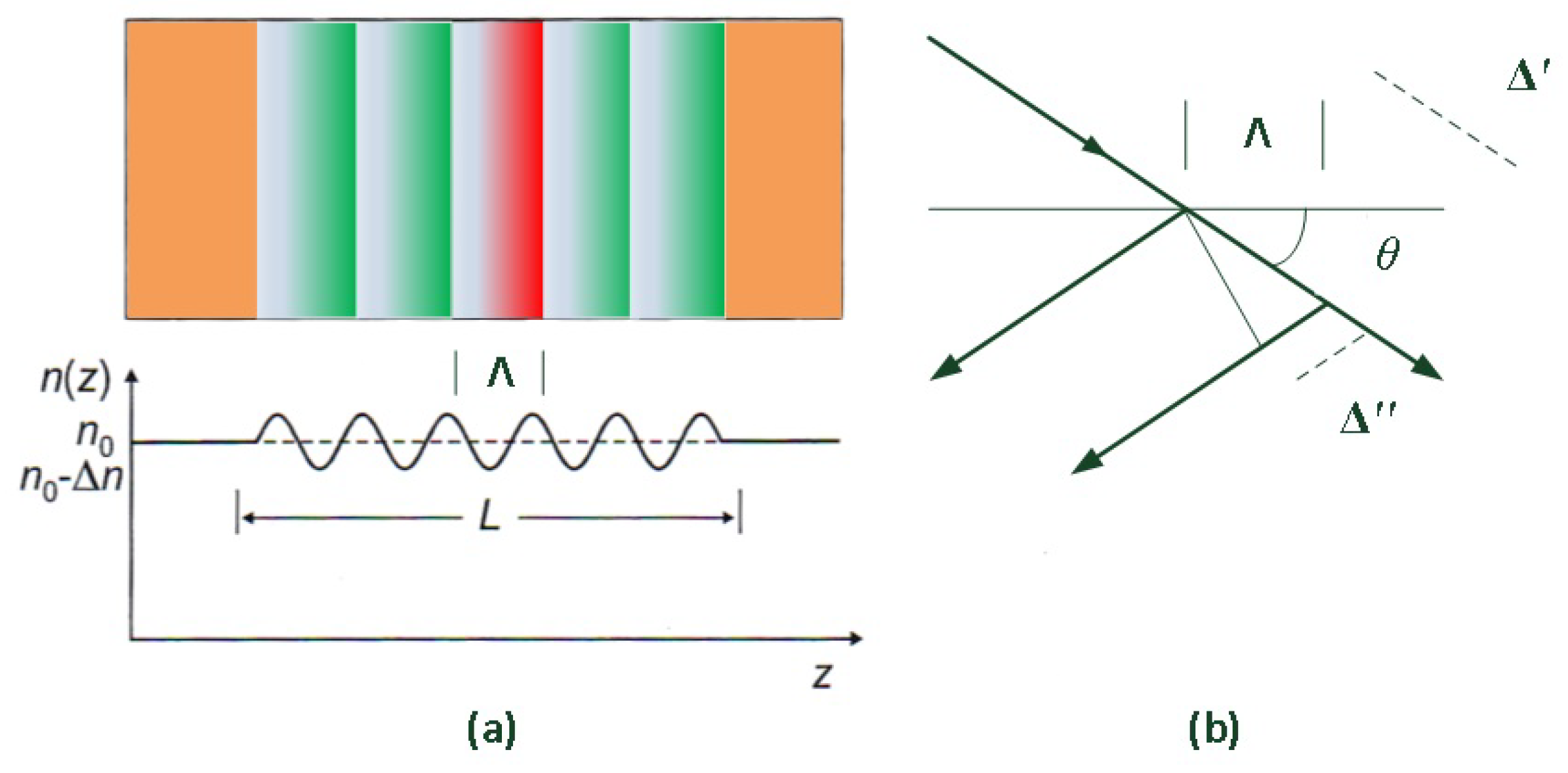
3. Fibre Bragg Grating

Fiber Bragg gratings are optical interference filters which are inserted in a glass carrier. They are composed of dielectric layers with alternating high and low refractive index. The thickness of the layers is selected so that partially reflected light waves constructively interfere at the interfaces of the layers. The refractive index provides a sinusoidal relationship of
n ( z ) = n 0 + Δ n sin 2 π Λ z ,
which can be periodically varied. Λ is the period length, Δ n is the modulation amplitude and n 0 is the average refractive index in the modulated range. Figure 3 shows the schematic structure together with the description of the path difference in an FBG. When a light wave of higher refractive index enters, it is partially reflected, and this reflection becomes maximum when the phase difference between the waves is a multiple of the wavelength. In the case of an FBG, the path difference becomes
Δ = 2 Λ cos θ .
This leads to the Bragg condition,
2 n 0 Λ cos θ = m λ m , m = 1 , 2 , 3 , ,
where Λ is a given lattice constant, θ is the angle of incidence, and λ m is the wavelength at which the reflection is maximum. The sinusoidal refractive index profile can be viewed for the first order m = 1 , from where the Bragg wavelength condition can be calculated as
λ B = 2 n 0 Λ cos θ .
The Bragg wavelength λ B is highly dependent on external influences. Mechanical elongation and temperature change Δ T particularly affect the Bragg wavelength. As a simple approximation, this dependence can be stated as
Δ λ B λ B = C S ε S + C T Δ T ,
where C S is the strain sensitivity, C T is the temperature coefficient, and ε S = Δ L L is the relative elongation of the fibre [46].
The strain may be used as an adjustable parameter for the fibre Bragg grating. This dependence of the Bragg wavelength is used to realize the concept as a tunable optical filter [40,41,47]. In the course of the work, however, the temperature effects are not negligible, and represent a particular challenge in terms of control.
The FBGs have an important function in the system design, as they help to form narrowband wavelength selective mirrors in the system. These are needed to generate the two laser modes (wavelengths) with the semiconductor optical amplifier. Therefore, the special structure of the FBGs used is presented here, and afterwards, how they are controlled in the overall system.
The internal structure of the tunable FBG from Advanced Optics Solutions [48] is schematically shown in Figure 4. The FBG is embedded into a holding device whose length can be controlled (stretched or elongated) by a stepper motor. As shown in Equation (5), the Bragg wavelength is dependent on the elongation of the fibre. From the rotation of the stepper motor, this results in a direct change of the Bragg wavelength. An integrated controller realizes the communication between the stepper motor (through the stepper motor’s driver) and a computer. This system is used as an interface to the Universal Serial Bus (USB).
Due to the high temperature sensitivity of FBGs (again in accordance with Equation (5)), there is additionally a temperature sensor in the housing of the adjustable FBG (not shown in Figure 4), in order to allow temperature compensation. The parameters of the temperature compensation can be determined by the vendor during its manufacturing phase, and stored in a look-up table [48,49,50]. The temperature compensation of the FBG used is therefore performed by calling a function and using the the look-up table that is provided by the vendor.
Furthermore, two protective casings serve as protection against over-stretching of the fibre and thereby ensure safety of the device during its operation. According to the manufacturer, the correct function of the light control over the FBG can be tested manually as follows.
  • Perform reference test.
  • Now the Position = 0.
  • Rotate about 200 steps in negative direction—no more!.
  • Here the light barrier (limit) triggers.
  • The position is now −200.
  • Now again perform reference test.
  • The position is again reset to 0.
This sequence is carried out automatically by the provided software when the Home function is called.

3.1. Operational Principle

The communication between the FBG and the computer is established via the serial USB 2.0 interface. To adjust the Bragg wavelength, a dynamic link library (DLL) is available. This contains various functions, which can step-wise measure and control the wavelength, temperature or speed. The manufacturer of the FBG, Advanced Optics Solutions GmbH has a software which is developed for this purpose and can be controlled directly [50]. Using this software, the Bragg wavelength can be adjusted through the speed of the stepper motor (for stretching or compressing). In addition, a temperature compensation mechanism in the software is implemented, through which the set Bragg wavelength is monitored every 60 s, depending on the temperature, and adjusts with the help of a compensation function underneath.
For an automated control in the overall system, the software of Advanced Optics Solutions can not be used because no programming interfaces are available. For this reason, the three main functions (setting the Bragg wavelength, controlling the speed control of the stepper motor, and temperature compensation) are simulated using the dynamic library in LabVIEW. LabVIEW is used for this purpose in version 18.0.1. [51], which recognizes the individual functions in the DLL and executes them appropriately.
Both for characterization and for use in the sensor setup, the FBG can be modelled by a series of parallel processes [52,53]. A process controls the setting of the Bragg wavelength, and the stepper motor speed, while the other process performs temperature compensation. Here, the Bragg wavelength is adjusted at any time, whereas after a certain time t K , a temperature compensation step is performed. For the laboratory setup, a time constant of t K = 45 s is used.
To model these parallel processes, it is suitable to use them particularly as descriptions of the discrete Petri net. With the possibility to run several states in Petri nets at the same time, this is preferred automatically by the state machines.

3.2. Modeling as a Petri Network

A very good introduction to the theory of Petri nets and a detailed derivation and description of the notation used thereby is given in [54]. A Petri network N is formally described by a six-tuple equation
N = ( P , T , A , ω , κ , M 0 ) ,
wherein,
P is a finite set of points in a graph, P = { p 1 , p 2 , . . . , p n } ,
T is a finite set of transitions T = { t 1 , t 2 , . . . , t n } ,
A ( P × T ) ( T × P ) is the flow relation for edge definition,
ω : A N is the weight function of the edges,
κ : P N is the capacity function of the task, and,
M 0 : P C { 0 } is the initial marking function.
As a model for the control of the FBG, the Petri net is used in Figure 5. It contains six points and six transitions. The initial marking of the graph is M 0 = ( 101000 ) . Mathematically, the graph in Figure 5 fully described by the so-called incidence matrix I FBG (Equation (7)) [54]. It specifies as to when and which value of weight can be provided to the transitions.
I FBG = 1 1 1 0 0 0 1 1 1 0 0 1 0 0 0 1 1 0 0 0 0 1 1 0 0 0 1 1 0 0 0 0 0 0 0 1
In the graph, …
p 1 : FBG is set to the idle/neutral state (available for adjusting the Bragg wavelength)
p 2 : FBG is set to a setting process
p 3 : OSA is in idle/neutral state and is ready to measure
p 4 : OSA is in measurement mode, waiting for the results
p 5 : Auxiliary/Help status for timeout
p 6 : FBG-Error due to its Bragg wavelength setting.
Since in a Petri network no fixed time for the switching behaviour of the transitions must be determined, this model can be universally used for the control. It first serves as a template for programming a control characterization and later as a model for the automated control of the overall system.

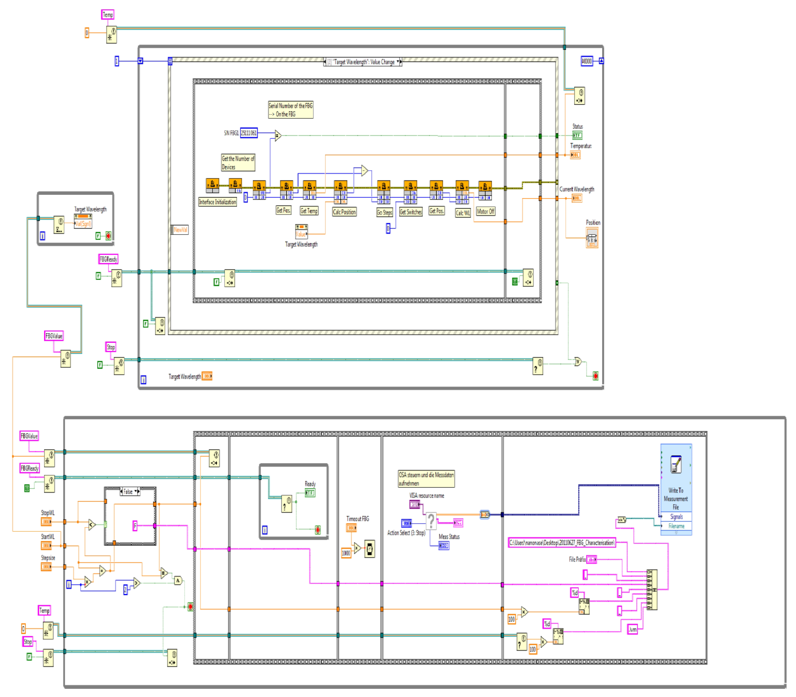
3.3. Implementation of the Control of the FBG in LabVIEW

As shown in the previous section, the control of fibre Bragg grating involves running two processes simultaneously. For the purpose of modelling this can be formally considered by a Petri net. In practical implementation, however, no real parallelism can be achieved for purely technical reasons. For instance, this is because of the fact that the serial USB interface already prevents the parallel communication. Since the FBG and the OSA are relatively slow with respect to the communication speed, a quasi-parallelism can be obtained. When programming, the so-called threats have to be used for practical purposes. These control the execution of multiple processes and thereby ensure an error-free communication.
In LabVIEW, the quasi-parallelism is easily performed by two separate loops [51,55]. This is why the complex representation of a pseudo code is not used at this point. Instead, the implementation of the Petri net in Figure 5 is shown as a characterization procedure of the fiber Bragg grating in the Appendix A in Figure A1.

3.4. Results of the Characterization of the FBG

In Figure 6, the results of measurements of three fibre Bragg grating are shown. It shows the comparison between the Bragg wavelength λ which is set by software and the actually measured Bragg wavelength λ which is measured at different points. A step size of 0.1 nm and 0.2 nm was chosen. For the sake of confirmation, reproducibility and accuracy, the latter was measured twice [56,57]. The curves marked in the legend with V and R represent the ascending (increase) and descending (decrease) in wavelength, respectively. The curves show here a linear dependence between the Bragg-wavelength-difference and the actually set wavelength. When the Bragg wavelength is set to 1538 nm, the deviation is between 0.1 and 0.25 nm. The minimum wavelength difference is reached when the FBG is working at about 1541 nm. If the Bragg wavelength is set to around 1546 nm, the actually measured wavelength is greater than the set one and a negative wavelength difference of up to −0.25 nm can be observed.
This behaviour could be caused by the control concept of the manufacturer. It is assumed that the fibre Bragg grating is optimized for the production of a working software [58], and a linear approximation around this regime is therefore, provided. Table 1, therefore, provides the parameters of the linearised curves that are shown in Figure 6. The slopes of all the curves are between 0.037 and 0.047. In view of these reasons, for the control of the fibre Bragg gratings in the overall system, this behaviour must be taken into account, which has been discussed in detail with the technical team of the vendor.

4. Variable Optical Coupler

Another essential component of the sensor system is the adjustable/variable optical coupler. It is used in the system in order to couple light from the broad-band resonator. This allows us to control the intensity of the modes that are generated by the respective fibre Bragg gratings. This is particularly important in order to artificially regulate the two modes to the same intensity. This means that the technical structure of the optical coupler used and its control should be discussed in detail.

4.1. Operation of the Tunable Optical Coupler Used

The general operation of an optical variable coupler is described here. By using a variable coupler it is possible to change the coupling length, and thus the coupling ratio. As a rule, this is achieved by a mechanical device. The coupler used by Evanescent Optics Inc. (Evanescent, Burlington, Canada) [49,59] serves two degrees of freedom; a micrometer screw in front of the coupler and a piezoelectric actuator.
The polished optical fibres are hereby inserted into a carrier (casing) plate. These support plates allow a transverse adjustment of the fibres, and, resulting in the displacement of the separating distance between the two fibre cores. An additional layer of oil ensures a smooth movement of these carrier plates. The fact that whether this oil also serves as a ‘matching oil’ between the polished fibres [60], cannot be answered on the basis of the manufacturer’s information.
The micrometer rotation is transmitted to the carrier plates as a transverse movement via a toggle system. This means that upon rotation of the micrometer screw to 0.0254 mm, a transverse displacement of one of the two carrier plates to about 1 μ m takes place [52]. This changes the distance between the two fibre cores and thus the coupling ratio.
This type of approach has a few limitations. The coupling ratio is defined by the use of a toggle lever system with a mechanical slot and associated with a hysteresis phenomenon. This is reinforced by additional hysteresis effects of the piezo-actuator. Thus, one can assign a specific micrometer position or input voltage, but not a fixed coupling ratio. Furthermore, the coupler is not suitable for fast switching. According to the manufacturer, generating a 1 Hz square-wave signal is still possible [52,61], but a filter with a time constant of 20 ms is integrated in the piezo-controller. Although this filter is a limiting factor for later miniaturization, it can be neglected in further consideration at this level, since it is significantly faster in the laboratory than the spectrum analyzer [47] which is being used in the laboratory.

4.2. Controlling the Variable Optical Coupler

The control of the actuator is accomplished by applying a voltage between 0 and 150 V. The voltage is provided by controller 914-2 made by the company [52] Evanescent Optics Inc. The coupler is connected to the controller at the output of piezoelectric (output port 916). In order to control the piezo-controller, a voltage between 0 and 5 V is required. This is done by the data acquisition device LabJack U3-HV, provided by the same company LabJack Corporation [51]. The analog output DAC0 by LabJack U3-HV is used. The maximum output voltage is 5 V with a resolution of 10 bits. This corresponds to a minimum possible resolution of about 4.9 mV. The output voltage of the LabJack is controlled by a dynamic library (DLL) specified by the manufacturer. Through the LabVIEW graphical user interface, the library is included in the programming environment and run on a Windows computer.
A simplified diagram of the structure for control and characterization of the variable coupler is shown in Figure 7. The three outputs of the optical coupler (TP = Transmission port CP = coupling port, Back = feedback port) can be connected alternately to an optical spectrum analyzer (OSA). Yokogawa 6370C is used as a spectrum analyzer [47]. The spectral wavelength range is from 600 nm to 1700 nm, with a resolution of 0.02 nm and a dynamic range of 78 dB. The spectrum analyzer is connected via the General Purpose Interface Bus (GPIB) and Agilent USB/GPIB adapter to a Windows computer.
For a complete characterization of the optical coupler, measurements are carried out on all three connecting ports with variation of both degrees of freedom. The scale of the micrometer screw is divided into 10 sub-blocks, each of 25 units. This results in 250 units of the micrometer screw. Since an exact conversion of these units is not known, they are referred to as arbitrary unit, abbreviated as [a.u.]. The starting point for the characterization is when the micrometer screw is turned to the extent that almost all division lines under the screw are covered. When the coupler is now used, about 10 to 15 units of the first sub-block are still visible.
The characterized area of the coupler was chosen between 15 a.u. and 165 a.u. The increment of the micrometer screw depends on the required resolution such as ten, five or two a.u. With each selected micrometer setting, the output voltage of the LabJack U3 is tuned such that the control voltage of the piezo-controller is between zero and four volts. For this purpose, the voltage is varied linearly between zero and four volts, increasing from four to zero volts and decreasing from four to zero volts, maintaining a step size of 0.1 V either way.
Measuring the output power at the terminals TP, CP and Back (see Figure 7) is carried out separately and one after the other with the help of spectrum analyzer. The measurement can be interpreted as a type of procedure, shown as a pseudo-code in Algorithm 1.
Algorithm 1: Pseudocode for the characterization procedure of an optical coupler
1: Define φ M Start , φ M Stop , φ M Step , U K Start , U K Stop , U K Step R +
2: for φ M Set = φ M Start , φ M Start + φ M Step , . . . , φ M Stop , do
3:      Turn Micrometer screw manually to φ M Set
4:      for  P o r t = T P , C P , B a c k do
5:         Connect P o r t with OSA
6:         for  U K Set = U K Start , U K Start + U K Step , . . . , U K Stop , do
7:             Send U K Set to DAC (e.g., LabJack U3)
8:             Wait until the Piezocontroller stops
9:             Measure the Spectrum (OSA)
10:             Transfer the Spectrum → Computer
11:         end for
12:      end for
13: end for
The evaluation of the measured values was done using the scripting language Python (version 3.8) [62,63,64] together with the packages NumPy 1.5.1, SciPy 1.19.0 and matplotlib 1.0.1.

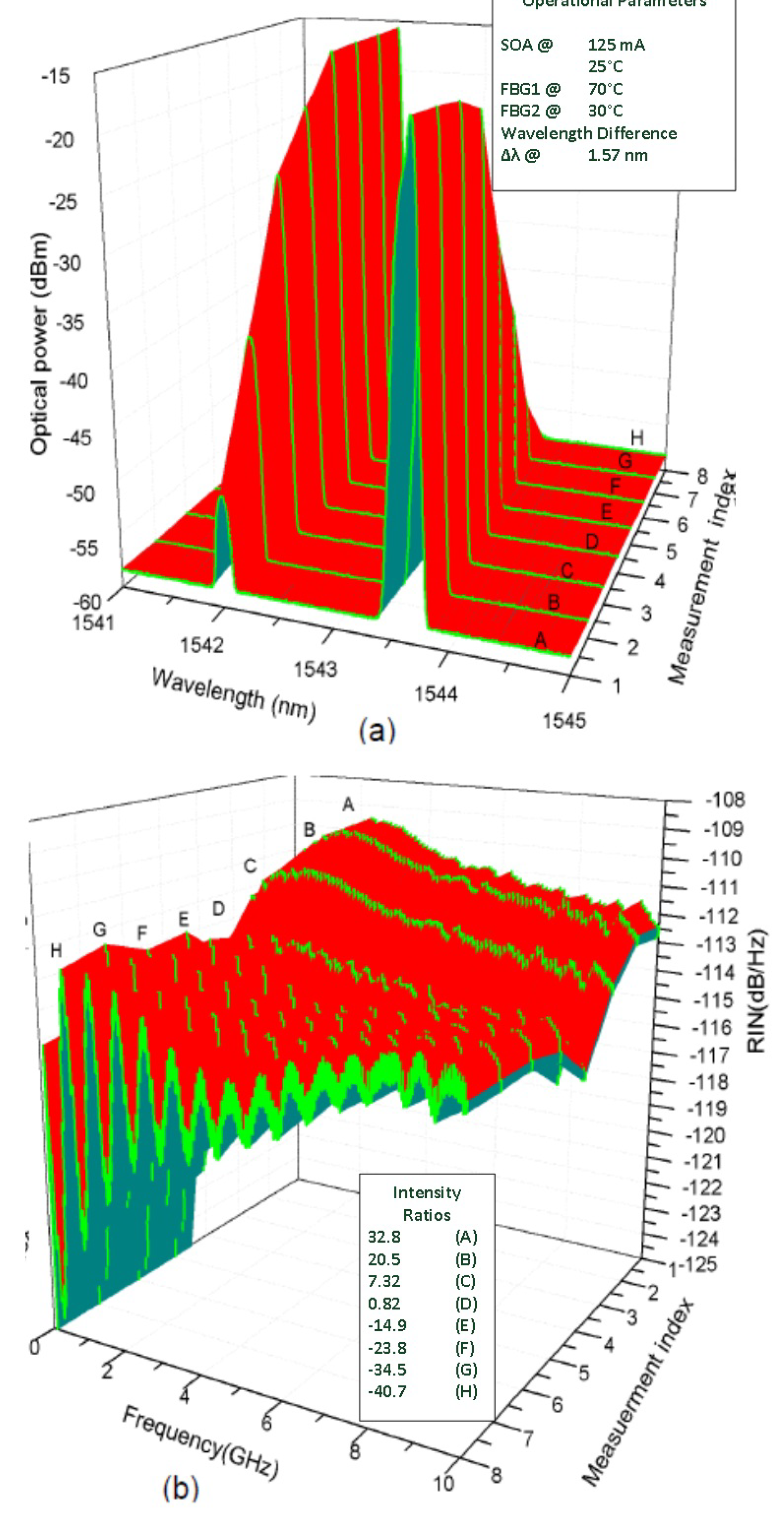
4.3. Results of Characterization of the Optical Coupler

Figure 8 shows the maximum output of the coupler as a function of the micrometer screw and the control voltage. The black curves show the behaviour of the CP-ports and the gray curves that of the TP port. For the sake of clarity, the back-port is not shown in these figures.
If no control voltage is applied and the micrometer screw is turned, the coupler exhibits a behaviour similar to that described in the literature [17,52]. The TP port falls while the CP port rises. This behaviour is well described by the couple-mode theory. There is another observable effect in Figure 8. There are two local maxima of the CP port or two local minima of the TP port. At this moment, where these effects come from could not be clarified within the scope of this work.
Further, the output power at the micrometer screw position 134 is also marked in Figure 8. This curve represents the working range of the optical coupler used. At this point it is the best transfer behaviour for this work.
The shape of the curves varies depending on whether the control voltage increases or decreases. Figure 9 shows the coupling ratio for three different wavelengths. It can be seen that the starting behaviour of the TP and CP of ports has a significant hysteresis. The threshold value of the hysteresis is about 1 V for both outputs. The hysteresis effect is so strong that it can not be neglected in an automated control or regulation. In addition, the coupler cannot be operated with a simple pilot control, since the hysteresis changes depending on the micrometer position, the input power and time. For an accurate setting of the coupling ratio, it is therefore necessary to measure the output power and readjust it in a control loop.

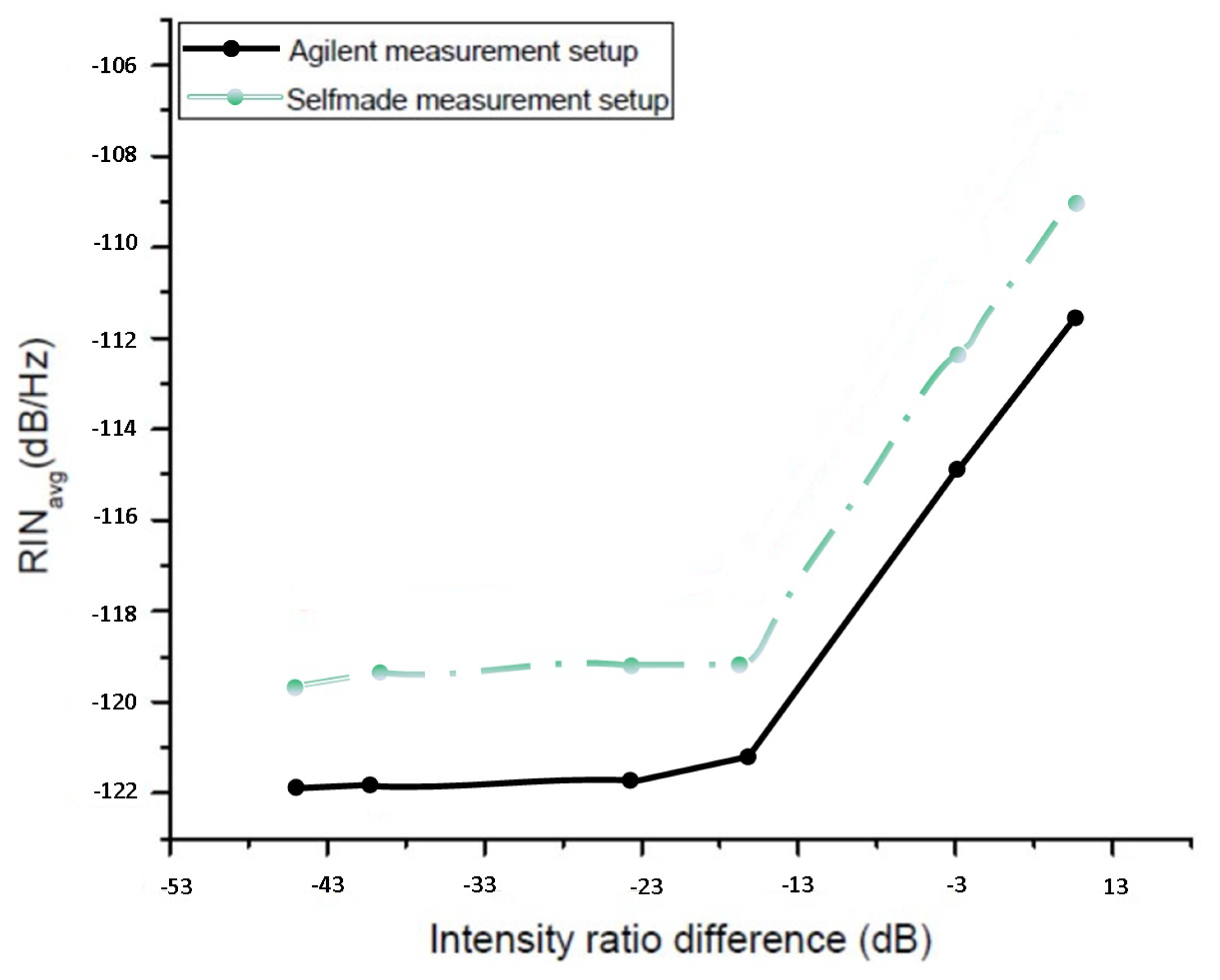
5. Comparison of RIN Results

A correlation between the noise outcomes of the current system with those from the Agilent existing system [65] will now be established. The temperature of the optical amplifier is kept at 25 C, and its current is increased from 110 to 125 mA, and the resulting situation is depicted in Figure 10. One of the scenarios is depicted in Figure 11 when the SOA is operated at 125 mA and 25 C. Because of this arrangement, we could sustain a wavelength difference Δ λ of 1.57 nm which was previously not possible. With the help of VCo, the value of the intensity ratio between both modes is changed. It is observed that the intensity of the outer mode Mo lessens in contrast to the intensity of the inner mode Mi. This in turn starts reducing the value of RIN accordingly, and the trend continues till the condition of mode equilibrium is reached (both modes with same intensities). When the intensity of the outer mode Mo is still decreased, the value of RIN reduces. This value of RIN waivers constantly between 4.7 and 5.3 GHz. A significant variation in RIN mirrors an undamped relaxation oscillation frequency, probably because of the unstable laser condition (sensor threshold due to SOA’s limits).
A view of the experimental outcomes from this investigation is provided in Figure 12 that mirrors worthwhile distinction. The magnitude of average RIN is significantly more for our experimental system. In other words, we can state with confidence that our setup gives precise and accurate data in terms of sensitivity when implemented. This is a very desirable trait for any biomedical application. As a result, our results are in complete agreement with with the ones that we have investigated and presented in this context, on simultaneous grounds [66].

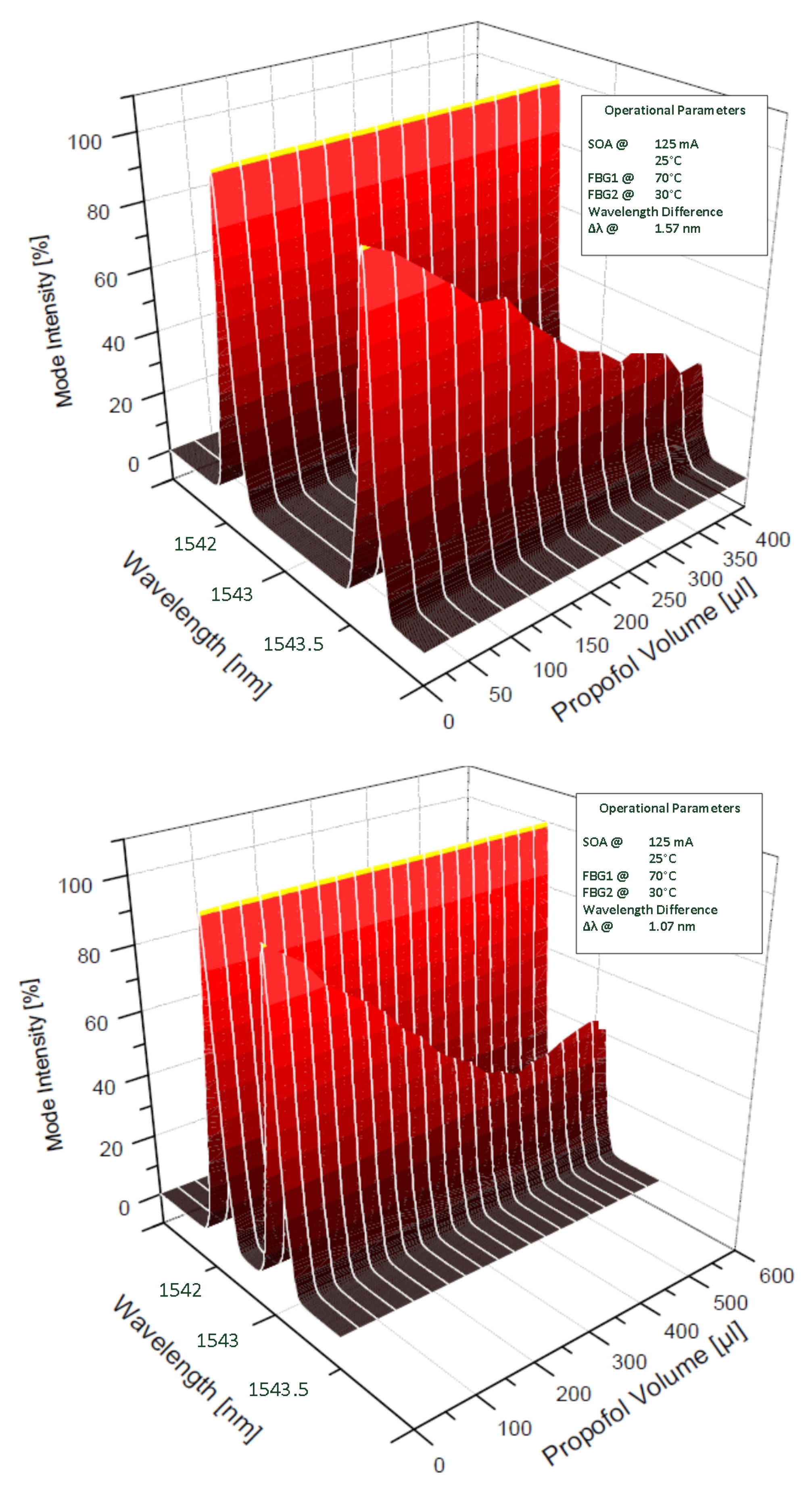
6. Measurements with Substances

After the characterization and calibration of the system, said system is used to analyze the substances. The sample holder is cleaned using Propanol [67,68], followed by a spray of nitrogen gas, in order to ensure non-presence of any contamination. This is essential for reliable and accurate measurements, and must be done before the commencement of each experimentation with a different substance.
A prescribed amount of Dichloro Methane (DCM), 1 mL, is inserted in the sample holder. Both FBGs are kept at the same mode spacing, where the entire procedure was formerly done. With the help of the coupler, the intensity of both modes is kept at equilibrium. We use propofol as the substance, and is gradually inserted in the sample holder (that contains DCM) with a pipette. The optical output of the system is observed on the OSA before and after inserting the substance, respectively, and the changed spectrum is recorded. The amount of propofol is now increased on a continual basis, and the resulting spectra are recorded, respectively. It is worth mentioning at this point that the substances have been taken out of the refrigerator, and kept at normal temperature for some time, before commencing with the experimentation. The complete procedure is repeated three times, for the sake of consistency, and the results were averaged.
The mode intensity is plotted against wavelength, for increasing amount of propofol in Figure 13. The first one shows the results at a mode spacing of 1.57 nm, whereas the second one shows the outcomes at 1.07 nm. Since the amount of light output from coupler VCi remains the same for both modes, keeping into consideration the effect of inner cavity, the graphs are scaled to the highest value of Mi. It is observed that Mo subsides as compared to Mi. This subsiding behaviour of Mo does not show a significantly non-linear effect, and the value of its Full Width at Half-Maximum does not show any alteration throughout this trend. After a certain point, the magnitude of Mo shows a slight rise. This originates from mode competition, and is in accordance with the cavity optomechanics effect. After a discussion with the technical team and two vendors of the OSA and the photodiode, this can be interpreted as follows. The spectrum contains specific absorption lines, and the width of each line is less than the Full Width at Half-Maximum of the complete wavelength range under investigation. This could account for one of the effects that the magnitude of the outer mode Mo tends to rise at the end. Next, a photodetector is a diode operated in reverse, used to measure the light in terms of current. It is manufactured for an entire series of wavelengths, instead of a specific one, unless it is specifically designed for a very particular application that involves only one wavelength. For these reasons, the behaviour of Mo changes with the mode spacing (difference between the wavelengths of both modes), in the presence of propofol, with a slight rise in its magnitude at the end.
Let us check the response of the sensor system when the amount of propofol is varied. Corresponding to the values of two mode spacing in Figure 13, the area under the curve for each mode is calculated and then the ratio between these values for both modes Mo and Mi is found, and plotted. This procedure is done separately for the mode spacing of 1.57 nm and 1.07 nm, respectively. To further enhance the procedure, the ratio of peak values of both modes at the same values of mode spacing (1.57 and 1.07 nm) is found, and their ratios are calculated, i.e., ratio of peak value of Mo to peak value of Mi. These values are plotted in the same graph in Figure 14, with increasing values of molarity (moles per litre). These experiments have been performed with varying substance quantity and SOA current, we obtain the same output for these two techniques to analyze the mode intensity ratio. In other words, the Full-Width at half maximum shows no dependence and stays the same when the values of intensity are varied under different absoprtion conditions, a highly desirable fact for the anticipated biomedical sensor. This can be further enhanced by investigating the absorption lines independently, for which a much sensitive and expensive device would be required, as the photodetector is not technically capable of performing that task.
The detection of propofol can be done through single mode spectroscopic techniques. Using paper spray ionization-mass spectrometry [69], this anesthetic drug has been detected in blood sample by mixing it with methanol and dimethylphenol, and using the extraction principle later afterwards with significant time slots. This involves expensive chemical substances, as well as non-economical precipitating and vortexing equipment that leads to infusion of these concentrations. In contrast, our method just utilizes two FBGs and laser system to conduct the complete experimentation, within a small fraction of average time. Moreover, the curve in [69] is calibrated and linearized in the measurement range of 50–100 μ L, whereas it has a declining slope in this work, implying an increased sensitivity. In a similar manner, gas chromatography-mass spectrometry using selected-ion monitoring mode has been engaged for propofol detection in brain, liver and adipose tissue in post-mortem [70]. This technique targets post-death procedures, and produces calibrated results which are linearized in the range of 50 and 500 μ L, with the limitation of limited precision for three targets in the body only, whereas our work produces the actual results with a steep slope in the same investigation regime. In another attempt, this agent has been detected in the exhaled human breath by photoacoustic spectroscopy and the investigated metabolites show interesting outcomes [71]. However, this has been done in the UV range, by using costly gadgets. Since we target to do it in the NIR, the components are not very expensive, thereby prioritizing the sanctity and cost-effectiveness of our method.

7. Conclusions

This work gives an investigation of a biomedical sensor for human well-being. In order for proper functioning of the sensor, the semiconductor arrangement should be examined for all the parts. Hereby, the FBGs have been examined in detail regarding their portrayal, adjustment and specialized investigation. Utilizing the algorithmic scheme for the specific device variables, the framework has been successfully analyzed in detail. The FBGs have been controlled via Petri network modelling scheme, and the measurement of wavelength difference between the set and Bragg wavelengths reveals negligibly small values.
Afterwards, the tunable coupler has been examined that controls the operation of the FBGs by a piezoelectric actuator and micrometer screw. The coupler has been thoroughly characterized by the schematic arrangement in Figure 7. This system is controlled by LabView, and the measurement scheme is implemented according to the pseudocode developed in Algorithm 1. This helps to analyze the maximum value of the output power of the coupler in relation to the position of the micrometer screw and the applied voltage. Since the sensor is destined for the wavelength regime in NIR, the coupling ratio is measured at three different wavelengths, namely 1542 nm, 1538 nm and 1546 nm, respectively. These results of the coupling ratio reveal that the wavelength-selective coupling is negligible, and can be used with complete accuracy for the biomedical sensor setup. A scenario with a wavelength difference of 1.57 nm has been investigated in detail, with a consistent output power, and the effect of various values of intensity ratio on RIN, thereby justifying the sensitivity of the sensor’s operation, and providing highly reliable piece of information, likewise mentioned in [31].
A comparison of RIN results with earlier outcomes provides a close contrast between the values which is quite encouraging [17,72]. We now attempt to check the values of RIN at different values of SOA injection current and temperature. This would certainly help in maintaining the sanctity of the results, thereby providing the biomedical sensor with optimal accuracy during its operation. As remarked earlier, since the modes are highly sensitive, we plan to use metamaterials in the future to confine them in our nanocavity. In this perspective, the setup would be amended with the aid of Metal Insulator Metal Insulator (MIMI) structures that could supposedly assist in the coupling and confining gap surface plasmons trough the evanescent wave which produced by surface plasmon polaritons, using the techniques that have been nicely developed in [26,27].

Author Contributions

Conceptualization, U.M.; methodology, U.M. and S.N.; software, F.A. and A.Z.; validation, U.M.; formal analysis, U.M. and F.A.; investigation, U.M. and U.G.; resources, U.M., F.A. and U.G.; data curation, U.M. and F.A., writing—original draft, U.M. and F.A.; writing—review and editing; U.M., F.A., M.R.A., H.E., Y.K., M.K.E., M.A.Q., A.A., S.N. and U.G.; visualization, U.M.; supervision, U.M. All authors have read and agreed to the published version of the manuscript.

Funding

This research received no external funding.

Institutional Review Board Statement

Not applicable.

Informed Consent Statement

Not applicable.

Data Availability Statement

Not applicable.

Acknowledgments

The authors are greatly indebted to the vendors of the equipment involved, as well as the technical team in our clean room, for providing worthwhile suggestions and moral support during the entire work.

Conflicts of Interest

The authors declare no conflict of interest.

Appendix A

Figure A1. LabVIEW program for the characterization of Fibre Bragg Grating.
Applsci 12 01856 g0a1
Table A1. List of symbols.
OSAOptical Spectrum Analyzer
ESAElectrical Spectrum Analyzer
SOASemiconductor Optical Amplifier
FBGFibre Bragg Grating
DMMDigital Multimeter
LDCLaser Diode Controller
RINRelative Intensity Noise
LNALow Noise Amplifier
MSEMean Square Error
VCi/VC1Variable Coupler corresponding to the inner cavity
VCo/VC2Variable Coupler corresponding to the outer cavity
Mi/M1Mode corresponding to the inner cavity
Mo/M2Mode corresponding to the outer cavity
Kappa κ capacity function of the task
λ wavelength of light
λ B Bragg wavelength
ω angular frequency
TP, CP, BackCoupler ports
Λ period length
Δ n modulation amplitude
n 0 average refractive index
C S strain sensitivity
C T temperature coefficient
ε S relative elongation of the fibre
NPetri network
Pfinite set of points in a graph
Tfinite set of transitions
ω weight function of the edges
M 0 initial marking function

References

  1. Cassone, G.; Trusso, S.; Sponer, J.; Saija, F. Electric Field and Temperature Effects on the Ab Initio Spectroscopy of Liquid Methanol. Appl. Sci. 2021, 11, 5457. [Google Scholar] [CrossRef]
  2. Vizbaras, A.; Šimonytė, I.; Droz, S.; Torcheboeuf, N.; Miasojedovas, A.; Trinkūnas, A.; Bučiūnas, T.; Dambrauskas, Ž.; Gulbinas, A.; Boiko, D.L.; et al. GaSb Swept-Wavelength Lasers for Biomedical Sensing Applications. IEEE J. Sel. Top. Quantum Electron. 2019, 25, 1501812. [Google Scholar] [CrossRef]
  3. Genovese, M.; Gramegna, M. Quantum Correlations and Quantum Non-Locality: A Review and a Few New Ideas. Appl. Sci. 2019, 9, 5406. [Google Scholar] [CrossRef] [Green Version]
  4. Kipnoo, E.K.R.; Boiyo, D.K.; Isoe, G.M.; Chabata, T.V.; Gamatham, R.R.G.; Leitch, A.W.R.; Gibbon, T.B. Demonstration of Raman-based dispersion-managed VCSEL technology for fibre-to-the-hut application. Opt. Fibre Technol. 2017, 34, 1–5. [Google Scholar] [CrossRef]
  5. Bader, F.; Jagtap, S. Chapter 10—Internet of Things-Linked Wearable Devices for Managing Food Safety in the Healthcare Sector. In Advances in Ubiquitous Sensing Applications for Healthcare, Wearable and Implantable Medical Devices; Dey, N., Ashour, A.S., Fong, S.J., Bhatt, C., Eds.; Academic Press: Loughborough, UK, 2020; Volume 7, pp. 229–253. ISBN 9780128153697. [Google Scholar] [CrossRef]
  6. Han, H.; Jung, D.-H.; Kim, H.-J.; Lee, T.S.; Kim, H.S.; Kim, H.; Park, S.H. Application of a Spectroscopic Analysis-Based Portable Sensor for Phosphate Quantitation in Hydroponic Solutions. J. Sens. 2020, 2020, 9251416. [Google Scholar] [CrossRef]
  7. Stephen, J. Harris Intracavity laser spectroscopy: An old field with new prospects for combustion diagnostics. Appl. Opt. 1984, 23, 1311–1318. [Google Scholar]
  8. Joindot, I. Measurements of relative intensity noise (RIN) in semiconductor lasers. J. Phys. III 1992, 2, 1591–1603. [Google Scholar] [CrossRef]
  9. Govind, P. Agrawal, Fiber Optic Communication Systems; Wiley Interscience: New York, NY, USA, 2002. [Google Scholar]
  10. Bock, C.; Prat, J. WDM/TDM PON Experiments using the AWG Free Spectral Range Periodicity to Transmit Unicast and Multicast Data. Optical Society of America (OSA). Opt. Express 2005, 13, 2887–2891. [Google Scholar] [CrossRef]
  11. Fox, M. Quantum Optics an Introduction; Oxford University Press Inc.: New York, NY, USA, 2006. [Google Scholar]
  12. Cho, B.I. X-ray Spectroscopies of High Energy Density Matter Created with X-ray Free Electron Lasers. Appl. Sci. 2019, 9, 4812. [Google Scholar] [CrossRef] [Green Version]
  13. Bacco, M.; Delmastro, F.; Ferro, E.; Gotta, A. Environmental Monitoring for Smart Cities. IEEE Sens. J. 2017, 17, 7767–7774. [Google Scholar] [CrossRef]
  14. Hart, J.K.; Martinez, K. Environmental Sensor Networks: A revolution in the earth system science? Earth-Sci. Rev. 2006, 78, 177–191. [Google Scholar] [CrossRef] [Green Version]
  15. Masud, U. Investigations on Highly Sensitive Optical Semiconductor Laser Based Sensorics for Medical and Environmental Applications: The Nanonose; Kassel University Press: Kassel, Germany, 2015; ISBN 3862195554. [Google Scholar]
  16. Parker, M.A. Physics of Optoelectronics; Taylor and Francis Group: Boca Raton, FL, USA, 2005. [Google Scholar]
  17. Masud, U.; Baig, M.I. Investigation of Cavity Length and Mode Spacing Effects in Dual-Mode Sensor. IEEE Sens. J. 2018, 18, 2737–2743. [Google Scholar] [CrossRef]
  18. Wang, Q.; Wang, Z.; Ren, W. Theoretical and Experimental Investigation of Fiber-Ring Laser Intracavity Photoacoustic Spectroscopy (FLI-PAS) for Acetylene Detection. J. Light. Technol. 2017, 35, 4519–4525. [Google Scholar] [CrossRef]
  19. Demtröder, W. Laser Spectroscopy 2: Experimental Techniques; Springer: Berlin/Heidelberg, Germany, 2015; ISBN 978-3-662-44641-6. [Google Scholar] [CrossRef]
  20. Baev, V.; Latz, T.; Toschek, P. Laser intracavity absorption spectroscopy. Appl. Phys. B 1999, 69, 171–202. [Google Scholar] [CrossRef]
  21. Kachanov, A.; Charvat, A.; Stoeckel, F. Intracavity laser spectroscopy with vibronic solid-state lasers. I. Spectrotemporal transient behavior of a Ti:sapphire laser. J. Opt. Soc. Am. B 1994, 11, 2412–2421. [Google Scholar] [CrossRef]
  22. Fomin, A.; Zavlev, T.; Rahinov, I.; Cheskis, S. A fiber laser intracavity absorption spectroscopy (FLICAS) sensor for simultaneous measurement of CO and CO2 concentrations and temperature. Sens. Actuators B Chem. 2015, 210, 431–438. [Google Scholar] [CrossRef]
  23. Liu, K.; Liu, T.; Jiang, J.; Peng, G.-D.; Zhang, H.; Jia, D.; Wang, Y.; Jing, W.; Zhang, Y. Investigation of wavelength modulation and wavelength sweep techniques in intracavity fiber laser for gas detection. J. Lightw. Technol. 2011, 29, 15–21. [Google Scholar]
  24. Bozóki, Z.; Sneider, J.; Szabó, G.; Miklós, A.; Serényi, M.; Nagy, G.; Fehér, M. Intracavity photoacoustic gas detection with an external cavity diode laser. Appl. Phys. B 1996, 63, 399–401. [Google Scholar] [CrossRef]
  25. Hodgkinson, J.; Tatam, R.P. Optical gas sensing: A review. Meas. Sci. Technol. 2012, 24, 012004. [Google Scholar] [CrossRef] [Green Version]
  26. Lio, G.E.; Ferraro, A.; Ritacco, T.; Aceti, D.M.; De Luca, A.; Giocondo, M.; Caputo, R. Leveraging on ENZ Metamaterials to Achieve 2D and 3D Hyper-Resolution in Two-Photon Direct Laser Writing. Adv. Mater. 2021, 33, 2008644. [Google Scholar] [CrossRef]
  27. Lio, G.E.; Ferraro, A.; Giocondo, M.; Caputo, R.; De, A. Color Gamut Behavior in Epsilon Near-Zero Nanocavities during Propagation of Gap Surface Plasmons. Adv. Opt. Mater. 2020, 8, 2000487. [Google Scholar] [CrossRef]
  28. Zafar, M.F.; Masud, U. A Multiple-Bands Metamaterial Absorber Based in X, Ku and K-Band. Opt. Quantum Electron. 2021. [Google Scholar] [CrossRef]
  29. NIST Special Publication, ISSN: 1048-776X, OCLC Number: 18972013, Online Version: NIST Special Publication (OCoLC)551418859. Available online: https://catalog.lindahall.org/discovery/fulldisplay?docid=alma993797263405961&context=L&vid=01LINDAHALL_INST:LHL&lang=en&search_scope=MyInstitution&adaptor=Local%20Search%20Engine&tab=LibraryCatalog&query=title,exact,NBS%20Special%20publication%20 (accessed on 24 June 2020).
  30. Bakeev, K.A. Process Analytical Technology: Spectroscopic Tools and Implementation Strategies for the Chemical and Pharmaceutical Industries, 2nd ed.; Wiley: Oxford, UK, 2010; ISBN 978-0-470-68960-8. [Google Scholar]
  31. de la Torre, O.; Floris, I.; Sales, S.; Escaler, X. Fiber Bragg Grating Sensors for Underwater Vibration Measurement: Potential Hydropower Applications. Sensors 2021, 21, 4272. [Google Scholar] [CrossRef] [PubMed]
  32. Sahota, J.K.; Gupta, N.; Dhawan, D. Fiber Bragg grating sensors for monitoring of physical parameters: A comprehensive review. Opt. Eng. 2020, 59, 060901. [Google Scholar] [CrossRef]
  33. Mark, R. Fisher and Travis C. Burt Rapid, automated, quality control of diffraction grating efficiency. Proc. SPIE 2017, 10373, 103730O. [Google Scholar] [CrossRef]
  34. Kim, S.; Jeong, Y.; Kim, S.; Kwon, J.; Park, N.; Lee, B. Control of the characteristics of a long-period grating by cladding etching. Appl. Opt. 2000, 39, 2038–2042. [Google Scholar] [CrossRef]
  35. Thevenon, A.; Flam, J.; Laude, J.P.; Touzet, B.; Lerner, J.M. Aberration Corrected Plane Gratings. Proc. SPIE 1987, 815, 136145. [Google Scholar]
  36. Goldstein, S.A.; Walters, J.P. A Review of Considerations for High Fidelity Imaging of Laboratory Spectroscopic Sources—Parts 1 and 2. Spectrochim. Acta Part B At. Spectrosc. 1976, 31, 201–316. [Google Scholar] [CrossRef]
  37. Palmer, Christopher. 2020. Diffraction Grating Handbook, Eighth Edition. Available online: https://www.researchgate.net/publication/339913143_DIFFRACTION_GRATING_HANDBOOK_eighth_edition (accessed on 13 January 2022).
  38. López-Higuera, J.M.; Cobo, L.R.; Incera, A.Q.; Cobo, A. Fiber optic sensors in structural health monitoring. J. Light. Technol. 2011, 29, 587–608. [Google Scholar] [CrossRef]
  39. Masud, U.; Baig, M.I.; Zeeshan, A. Automatization analysis of the extremely sensitive laser-based dual-mode biomedical sensor. Lasers Med. Sci. 2020, 35, 1531–1542. [Google Scholar] [CrossRef]
  40. LM14S2—Universal 14-Pin Butterfly Laser Diode Mount, Thorlabs. Available online: https://www.thorlabs.com/thorproduct.cfm?partnumber=LM14S2 (accessed on 14 September 2019).
  41. LDC-3900 Modular 4-Channel Laser Diode Controller, Newport. Available online: https://www.newport.com/f/4-channel-modular-laser-diode-controller-ldc-3900 (accessed on 5 October 2018).
  42. Petermann, K. Laser Diode Modulation and Noise; Kluwer Academic Publishers: Amsterdam, The Netherlands, 1991. [Google Scholar]
  43. Agrawal, G.P.; Dutta, N.K. Semiconductors Lasers; Van Nostrand Reinhold: New York, NY, USA, 1993. [Google Scholar]
  44. Hui, R.; O’Sullivan, M. Fiber Optic Measurement Techniques; Elsevier Academic Press: Cambridge, MA, USA, 2009. [Google Scholar]
  45. Rohde & Schwarz: FSP30. Available online: https://www.rohde-schwarz.com/us/product/fsp-productstartpage_63493-8043.html (accessed on 2 May 2019).
  46. Dietrich, K. Optik—Grundlagen und Anwendungen, 2nd ed.; Verlag Harri Deutsch: Frankfurt, Germany, 2007; ISBN 978-3-8171-1741-3. [Google Scholar]
  47. AQ6370C Optical Spectrum Analyzer, Yokogawa. Available online: https://tmi.yokogawa.com/eu/solutions/products/optical-measuring-instruments/optical-spectrum-analyzer/aq6370c-optical-spectrum-analyzer/ (accessed on 2 March 2018).
  48. Advanced Optics Solutions. Available online: https://www.aos-fiber.com/eng/Products.html (accessed on 6 December 2020).
  49. Evanescent Optics Inc. Available online: http://www.evanescentoptics.com/products/ (accessed on 4 October 2020).
  50. Stepper Motor Tunable Fiber Bragg Grating—User Guide; AOS GmbH: Dresden, Germany, 2011.
  51. LabVIEW 2018 Service Pack 1 Readme for Windows. Available online: http://www.ni.com/pdf/manuals/374715k.html#known (accessed on 3 March 2019).
  52. Polarization Maintaining Variable Ratio Evanescent Wave Couplers, 2nd ed.; Evanescent Optics Inc.: Oakville, ON, Canada, 2009.
  53. Xia, Q.; Yuan, L.-M.; Chen, X.; Meng, L.; Huang, G. Analysis of Methanol Gasoline by ATR-FT-IR Spectroscopy. Appl. Sci. 2019, 9, 5336. [Google Scholar] [CrossRef] [Green Version]
  54. Christos, G. Cassandras; Stéphane Lafortune, Introduction to Discrete Event Systems; Springer: Boston, MA, USA, 2008; ISBN 978-0-387-33332-8. [Google Scholar] [CrossRef]
  55. Rodrigues, M.S.; Borges, J.; Lopes, C.; Pereira, R.M.S.; Vasilevskiy, M.I.; Vaz, F. Gas Sensors Based on Localized Surface Plasmon Resonances: Synthesis of Oxide Films with Embedded Metal Nanoparticles, Theory and Simulation, and Sensitivity Enhancement Strategies. Appl. Sci. 2021, 11, 5388. [Google Scholar] [CrossRef]
  56. Premaratne, M.; Lowery, A.J.; Ahmed, Z.; Novak, D. Modeling noise and modulation performance of Fiber grating external cavity lasers. IEEE J. Quantum Electron. 1997, 3, 290–303. [Google Scholar] [CrossRef] [Green Version]
  57. Jonas, A.; Stiel, H.; Glöggler, L.; Dahm, D.; Dammer, K.; Kanngießer, B.; Mantouvalou, I. Towards Poisson Noise Limited Optical Pump Soft X-ray Probe NEXAFS Spectroscopy Using a Laser-Produced Plasma Source. Opt. Express 2019, 27, 36524–36537. [Google Scholar] [CrossRef] [PubMed]
  58. O’Donnell, K.P.; Chen, X. Temperature dependence of semiconductor band gaps. Appl. Phys. Lett. 1991, 58, 2924–2926. [Google Scholar] [CrossRef] [Green Version]
  59. Digonnet, M.J.F.; Shaw, H.J. Analysis of a Tunable Single Mode Optical Fiber Coupler. IEEE Trans. Microw. Theory Tech. 1982, 30, 592–600. [Google Scholar] [CrossRef]
  60. Markatos, S.; Kerr, A.; Giles, I.P. Electrically Tunable Optical Fibre Polished Coupler. In Proceedings of the IEE Colloquium on All-Fibre Devices, London, UK, 3 June 1988; pp. 6/1–6/4. [Google Scholar]
  61. Nuno, B. Carvalho and Dominique Schreurs, Microwave and Wireless Measurement Techniques; Cambridge University Press: Cambridge, UK, 2013; pp. 63–89. ISBN 9781107004610. [Google Scholar]
  62. Python Developer’s Guide. Available online: devguide.python.org (accessed on 17 December 2019).
  63. Jarrod, M.K.; Michael, A. Python for Scientists and Engineers. Comput. Sci. Eng. 2011, 13, 9–12. [Google Scholar] [CrossRef] [Green Version]
  64. Matplotlib: Visualization with Python. Available online: https://matplotlib.org/ (accessed on 11 December 2019).
  65. Masud, U.; Ali, M.; Ikram, M. Calibration and stability of highly sensitive fibre based laser through relative intensity noise. Phys. Scr. 2020, 95, 055505. [Google Scholar] [CrossRef]
  66. Masud, U.; Jeribi, F.; Zeeshan, A.; Tahir, A.; Ali, M. Highly Sensitive Microsensor Based on Absorption Spectroscopy: Design Considerations for Optical Receiver. IEEE Access 2020, 8, 100212–100225. [Google Scholar] [CrossRef]
  67. Reed, M.D. Isopropanol. In Encyclopedia of Toxicology, 2nd ed.; Wexler, P., Ed.; Elsevier: Amsterdam, The Netherlands, 2005; pp. 653–655. ISBN 9780123694003. [Google Scholar] [CrossRef]
  68. Budić-Leto, I.; Humar, I.; Gajdoš Kljusurić, J.; Zdunić, G.; Zlatić, E. Free and Bound Volatile Aroma Compounds of ´Maraština´ Grapes as Influenced by Dehydration Techniques. Appl. Sci. 2020, 10, 8928. [Google Scholar] [CrossRef]
  69. Liu, Y.; Zhang, X.H.; Mi, W.D.; Zhou, Y.L.; Zhang, C.S.; Zhang, X.X. Rapid determination and continuous monitoring of propofol in microliter whole blood sample during anesthesia by paper spray ionization-mass spectrometry. Anal. Bioanal. Chem. 2021, 413, 279–287. [Google Scholar] [CrossRef] [PubMed]
  70. Hikiji, W.; Kudo, K.; Usumoto, Y.; Tsuji, A.; Ikeda, N. A simple and sensitive method for the determination of propofol in human solid tissues by gas chromatography-mass spectrometry. J. Anal. Toxicol. 2010, 34, 389–393. [Google Scholar] [CrossRef] [PubMed] [Green Version]
  71. Laurila, T.; Sorvajärvi, T.; Saarela, J.; Toivonen, J.; Wheeler, D.W.; Ciaffoni, L.; Ritchie, G.A.D.; Kaminski, C.F. Optical Detection of the Anesthetic Agent Propofol in the Gas Phase. Anal. Chem. 2011, 83, 3963–3967. [Google Scholar] [CrossRef] [PubMed]
  72. Masud, U.; Jeribi, F.; Alhameed, M.; Akram, F.; Tahir, A.; Naudhani, M.Y. Two-Mode Biomedical Sensor Build-up: Characterization of Optical Amplifier. Tech Sci. Comput. Mater. Contin. 2022, 70, 5487–5489. [Google Scholar] [CrossRef]
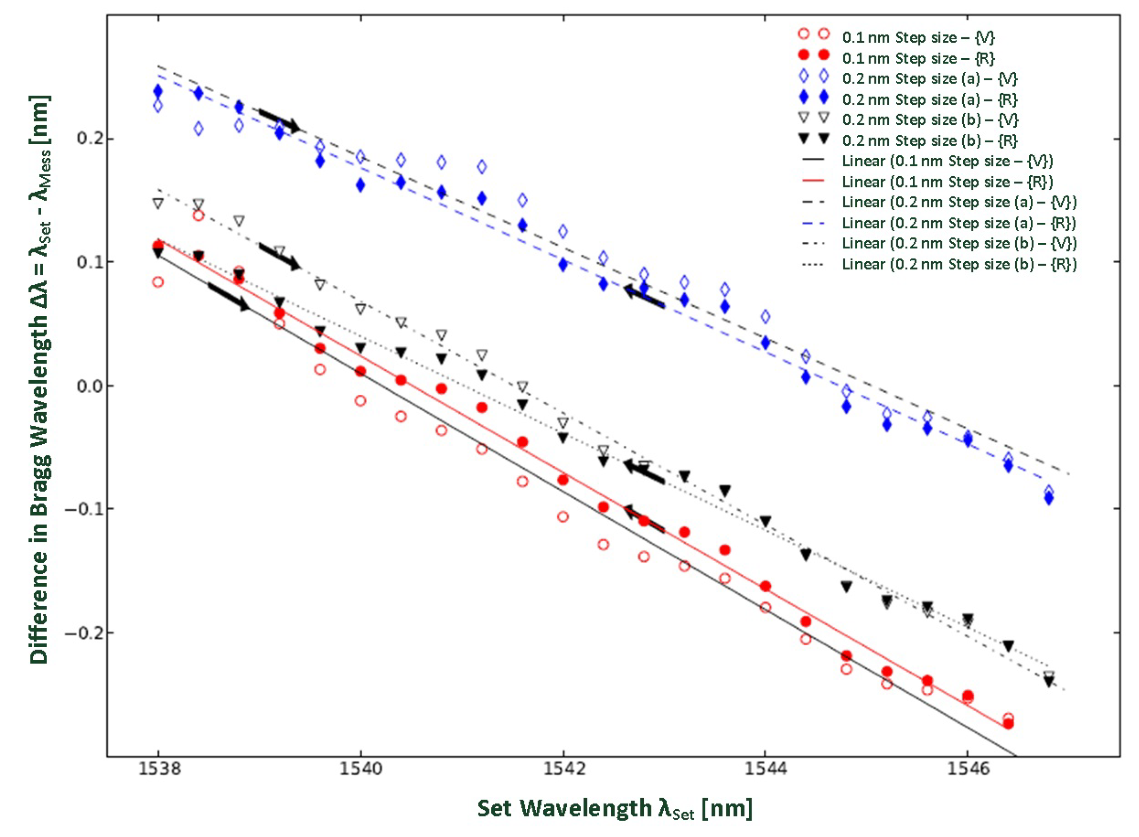
Figure 1. Experimental setup of the sensor laser under investigation, with the Fibre Bragg Gratings (FBGs), Semiconductor Optical Amplifier (SOA), Fixed/Variable Coupler (FC/VC), loop mirror, isolators (for light flow in single direction), Optical Spectrum Analyzer (OSA) and Collimator (for substance) (Reprinted with permission from [17], Copyright 2021 IEEE).
Applsci 12 01856 g001
Figure 2. Electrical output of the laser system, consisting of Optical Receiver (PIN-PhotoDiode (PD), Bias-Tee and Low Noise Amplifier (LNA)), Voltmeter and Electrical Measurement System (Electrical Spectrum Analyzer (ESA) or Oscilloscope).
Applsci 12 01856 g002
Figure 3. (a) Schematic representation of the FBG’s sinusoidal refractive index modulation of the length L. (b) The path difference is composed of the distances Δ and Δ , so that: Δ = Δ + Δ = 2 Λ cos θ .
Applsci 12 01856 g003
Figure 4. Schematic representation of the internal structure of the tunable fibre Bragg grating. The fibre Bragg grating fixed in a holder can be stretched or compressed by a stepper motor. As a result, the Bragg wavelength of the grating changes. The stepper motor is controlled via USB. Details of The protection mechanism can be found in [50].
Applsci 12 01856 g004
Figure 5. Petri network for modelling the parallel control of the FBG.
Applsci 12 01856 g005
Figure 6. Measurement of wavelength difference between the set and measured Bragg wavelengths.
Applsci 12 01856 g006
Figure 7. Schematic construction of measurement for characterization of tunable coupler.
Applsci 12 01856 g007
Figure 8. Representation of the maximum power output in dependence of the position of the micrometer screw and the control voltage. The color-coded line shows the relevant work area for this work.
Applsci 12 01856 g008
Figure 9. Coupling ratio of the transmission output at three wavelengths (1538, 1542 and 1546 nm). This evidence shows that the wavelength-selective coupling is negligible.
Applsci 12 01856 g009
Figure 10. Illustration of both modes’ existence for SOA at 25 C.
Applsci 12 01856 g010
Figure 11. Illustration of (a) mode competition in the setup, with SOA @125 mA and 25 C, FBGi @70 C, FBGo @30 C, and Δ λ of 1.57 nm, and, (b) corresponding RIN spectra under various intensity ratios Mi/Mo.
Applsci 12 01856 g011
Figure 12. Comparing average RIN from both measurement setups.
Applsci 12 01856 g012
Figure 13. Normalized output spectra of the laser system with absorption from Propofol (top) in 1 mL DCM at Δ λ = 1.57 nm and (bottom) in 1 mL DCM at Δ λ = 1.07 nm.
Applsci 12 01856 g013
Figure 14. Variation of the mode intensity ratio (Mo/Mi) with molarity at Δ λ = 1.57 nm and Δ λ = 1.07 nm, corresponding to the situations in Figure 13, respectively.
Applsci 12 01856 g014
Table 1. Parameters of the linearly adapted FBG difference characteristic curve. a is the slope and b is the intersection point at the y-axis. MSE is the mean squared error of the linearization.
No.Step SizeDirectionabMean Squared Error (MSE)
10.1 nmV−0.04873.62 0.0194
20.1 nmR−0.04772.70 0.0088
30.2 nm (a)V−0.03756068 0.0184
40.2 nm (a)R−0.03757.63 0.0107
50.2 nm (b)V−0.04569.73 0.0078
60.2 nm (b)R−0.03960.54 0.0090
Publisher’s Note: MDPI stays neutral with regard to jurisdictional claims in published maps and institutional affiliations.

