A Theoretical Approach to Ordinal Classification: Feature Space-Based Definition and Classifier-Independent Detection of Ordinal Class Structures

Abstract

Ordinal classification (OC) is a sub-discipline of multi-class classification (i.e., including at least three classes), in which the classes constitute an ordinal structure. Applications of ordinal classification can be found, for instance, in the medical field, e.g., with the class labels order, early stage-intermediate stage-final stage, corresponding to the task of classifying different stages of a certain disease. While the field of OC was continuously enhanced, e.g., by designing and adapting appropriate classification models as well as performance metrics, there is still a lack of a common mathematical definition for OC tasks. More precisely, in general, a classification task is defined as an OC task, solely based on the corresponding class label names. However, an ordinal class structure that is identified based on the class labels is not necessarily reflected in the corresponding feature space. In contrast, naturally any kind of multi-class classification task can consist of a set of arbitrary class labels that form an ordinal structure which can be observed in the current feature space. Based on this simple observation, in this work, we present our generalised approach towards an intuitive working definition for OC tasks, which is based on the corresponding feature space and allows a classifier-independent detection of ordinal class structures. To this end, we introduce and discuss novel, OC-specific theoretical concepts. Moreover, we validate our proposed working definition in combination with a set of traditionally ordinal and traditionally non-ordinal data sets, and provide the results of the corresponding detection algorithm. Additionally, we motivate our theoretical concepts, based on an illustrative evaluation of one of the oldest and most popular machine learning data sets, i.e., on the traditionally non-ordinal Fisher’s Iris data set.

1. Introduction

In the traditional sense, a multi-class classification task is denoted as an ordinal classification (OC) task if the corresponding class label names can be sorted, e.g., small ≺ medium ≺ large, or short ≺ medium ≺ long, etc. In this case, one can implement OC-specific classifiers to improve classification performance [1]. However, in general, a classification model can only benefit from a specific label order if it is represented in the corresponding feature space [2]. Otherwise, it can lead to a severely decreased classification performance [3].

Following the latest trend of (deep) artificial neural networks (ANNs) [4], less than one decade ago, researches started to adapt ANNs to the field of ordinal regression (OR), see, e.g., in [5,6]. For instance, different ANN architectures have been proposed for the interesting task of age estimation [7,8]. Note that ordinal classification constitutes a special case of ordinal regression. Furthermore, regularly, these terms are even used interchangeably, as, for instance, in one of the recent survey papers on OR [9].

Moreover, the evaluation of OC tasks requires a specific choice of performance metrics. For a broad overview on OC-specific performance measures, we refer the reader to the works in [10,11]. For instance, let us consider the misclassification of a person’s early stage of a severe disease as an intermediate stage, and the misclassification of the early stage as a final stage. In both cases, we obtain a classification error. However, obviously, with respect to a real-world application (e.g., the detection of a certain cancer stage), each of the errors should be associated with a different cost value.

Instead of restricting the field of OC to multi-class classification tasks in which the class label names constitute an ordinal structure, Lattke et al. proposed detecting ordinal class structures independently from the label names [3], based on classifier cascades [12], in combination with different classification models such as nearest neighbour classifiers [13], decision trees [14], or support vector machines (SVMs) [15,16]. Note that prior to the adaptation of (deep) ANNs, first the basic SVM model was adapted for the task of OC/OR [17,18,19].

On the one hand, the field of ordinal classification was steadily enriched by the introduction of OC-specific classification models, metrics, as well as modified ANN architectures, and on the other hand, we observed a lack for a common definition of OC tasks. Therefore, inspired by the cascades-based approach for the detection of ordinal class structures [3,20], recently, in [21], we proposed a working definition for OC tasks that is based on the relation between the pairwise performance of binary SVM models. Further investigations of our initially proposed working definition led us to a new theoretical concept, which allows us to provide a novel and generalised working definition that is not based on any classification/regression model.

Therefore, the current work constitutes a generalisation of our previous work [21]. In addition to the work in [21], here, we provide the following outcomes: (i) We introduce the concept of level of separability measures and ordinal arrangements; (ii) We provide a generalised working definition, based on the aforementioned concepts, which is independent from any classification model; (iii) We discuss additionally observed limitations of our initial working definition and extend Theorem 1 from our previous work [21] by Corollary 1; (iv) We introduce a classifier-independent measure, which allows us to find ordinal class structures, based solely on the corresponding feature space; (v) We evaluate our proposed generalised working definition on a set of traditionally ordinal, as well as traditionally non-ordinal data sets; and (vi) We discuss and illustrate the usefulness of our proposed working definition, based on the obtained outcomes, as well as on an additional motivational example.

Finally, note that by the term OC, throughout the whole work, we will refer to multi-class classification tasks (i.e., classification tasks with at least three classes) with an ordinal class structure. More precisely, including the term OC does not imply that the corresponding feature space is ordinal-scaled [22,23]. Moreover, even if one can apply different classification models to detect ordinal class structures, the detection of ordinal class structures itself is not part of the corresponding classification process. Figure 1 provides an exemplary pipeline for the processing steps of an arbitrary classification task, to emphasise the research area of the current contribution.

The remainder of this work is organised as follows. In Section 2, we first provide the formalisation of our approach, followed by our proposed feature space-based definition for ordinal classification tasks, which is based on specific mappings that we denote as level of separability measures (LSMs). Subsequently, in Section 3, we discuss the main differences to our recently provided working definition, and present additional characteristics of our current theoretical concepts. We introduce a specific LSM mapping in Section 4, including a numerical example as well as a simple illustration. In Section 5, we provide an experimental validation of our proposed feature space-based working definition for ordinal classification tasks, based on traditionally ordinal as well as traditionally non-ordinal data sets, including a running time evaluation. A detailed discussion on the complexity, limitations, and usefulness of our proposed working definition is followed in Section 6. Finally, in Section 7, we conclude the current work.

2. Formalisation and Generalised Working Definition for Ordinal Class Structures

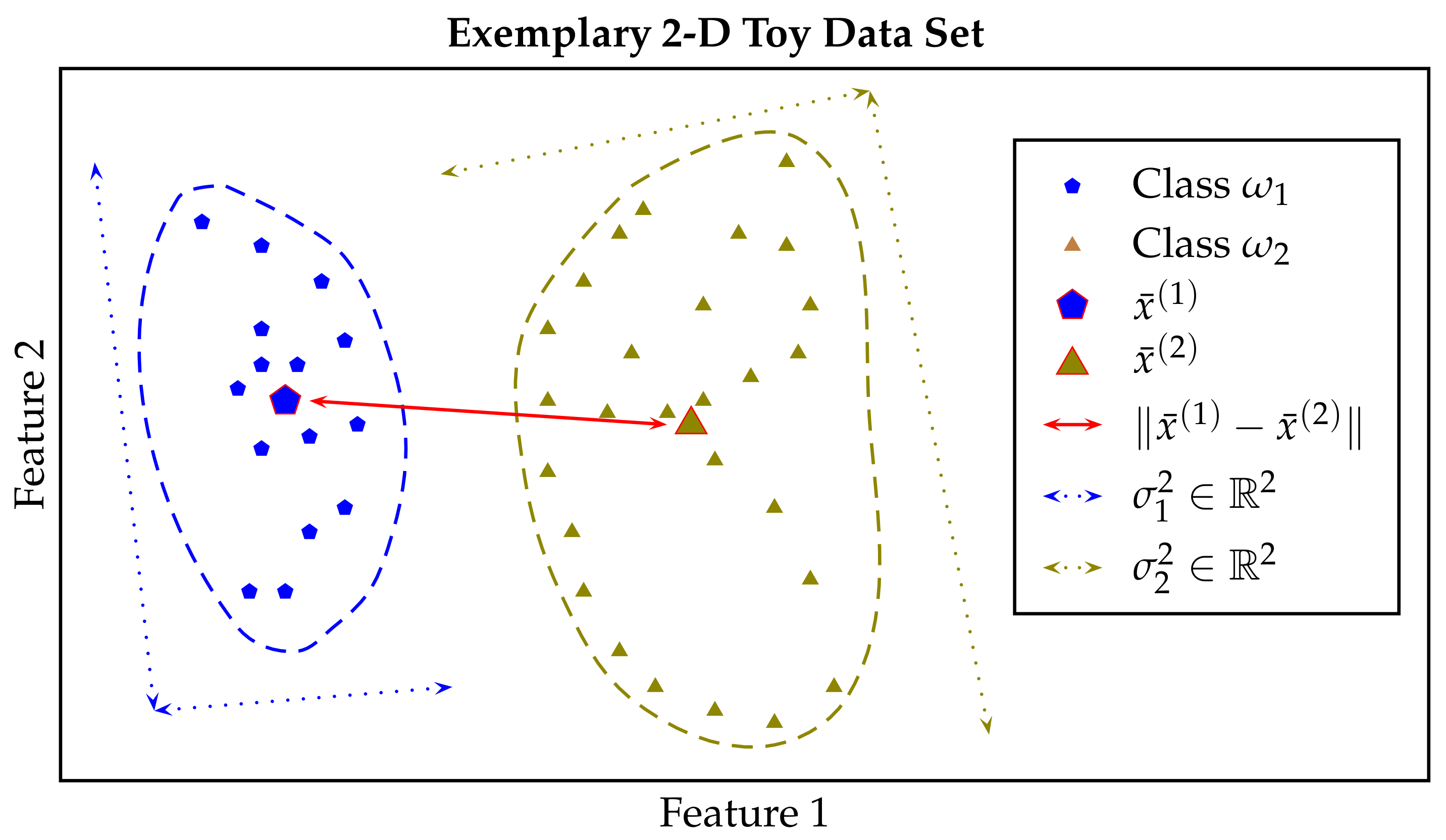
In this section, we will first provide the formalisation for our current work. Subsequently, we will introduce our proposed novel working definition for ordinal classification tasks that is independent from the meaning of the corresponding class labels.

2.1. Formalisation

Let $X_{\Omega }$ be a c-class classification task, which is defined by the d-dimensional data set $X\subset {\mathbb{R}}^d$, $d\in \mathbb{N}$, and the corresponding set of class labels $\Omega =\{{\omega }_1,\dots ,{\omega }_c\}$, with $c>2$. We denote the resulting index set as I, i.e., $I=\{1,\dots ,c\}$. Each element of $X_{\Omega }$ is a task-related object, which is a pair consisting of a data sample and its true class label, i.e., $X_{\Omega }={\left\{(x_i,y_i)\right\}}_{i=1}^N$, $y_i\in \Omega ,\forall i=1,\dots ,N$, whereby $N=|X_{\Omega }|$ denotes the number of elements in the set $X_{\Omega }$. Specifically, it holds, $X_{\Omega }⊊X\times \Omega$. Moreover, by $X_{\Omega }^{i,j}$, we denote the binary subtask that is restricted to the classes ${\omega }_i$ and ${\omega }_j$, i.e., for all $i,j\in I$, with $i\ne j$, we define

$$X_{\Omega }^{i,j}:=\{(x,y)\in X_{\Omega }|y={\omega }_i\vee y={\omega }_j\}.$$

(1)

Therefore, it holds that $X_{\Omega }^{i,j}=X_{\Omega }^{j,i},\forall i,j\in I,i\ne j$. For the definition of ordinal classification tasks, in this work, we introduce the term level of separability measures, which we define as follows, in Definition 1.

Definition 1

(Level of Separability Measures). Let $X_Y$, $X\subset {\mathbb{R}}^d$, $d\in \mathbb{N}$, and $Y=\{0,1\}$ constitute a binary classification task in a d-dimensional feature space. Furthermore, let $X_{\overline{Y}}$ be the corresponding binary classification task, where we interchange the class labels of all samples from the task $X_Y$, i.e., $X_{\overline{Y}}:=\left\{(x,1-y)\right|(x,y)\in X_Y\}$. Additionally, for each $X\subset {\mathbb{R}}^d$, we define the set $X_Y^{*}$ as $X_Y^{*}=X\times Y$. We denote the non-constant and non-randommapping μ as a level of separability measure (LSM), if μ fulfils the following properties:

$$\left.\begin{array}{ccccc}\hfill \left(\mathrm{P}0\right)& \mu \left(X_Y\right)\ge 0,\hfill & \hfill & \forall X_Y\subset {\mathbb{R}}^d\times \{0,1\},\hfill & \hfill \left(\mathrm{nonnegative}\right),\\ \hfill \left(\mathrm{P}1\right)& \mu \left(X_Y^{*}\right)\le \mu \left(Z_Y\right),\hfill & \hfill & \forall Z_Y\subset {\mathbb{R}}^d\times \{0,1\},X\subset {\mathbb{R}}^d,\hfill & \hfill \left(\mathrm{point-separating}\right),\\ \hfill \left(\mathrm{P}2\right)& \mu \left(X_Y\right)=\mu \left(X_{\overline{Y}}\right),\hfill & \hfill & \forall X_Y\subset {\mathbb{R}}^d\times \{0,1\},\hfill & \hfill \left(\mathrm{label\; invariant}\right).\end{array}\right\}$$

(2)

Note that a higher value for $\mu$ implies a higher level of separability. The properties defined in Equation (2) are further discussed in the following remark, i.e., in Remark 1.

Remark 1

(Properties of LSM mappings). Let μ be an LSM mapping by Definition 1. Furthermore, let $X_{\{0,1\}}\subset {\mathbb{R}}^d\times \{0,1\}$ constitute a binary classification task. Property (P1) of Equation (2) implies that if we set $Z=X_{\{0,1\}}^{*}=X\times \{0,1\}$, then the value of $\mu \left(Z\right)$ is equal to the minimum value of μ, across all $X_{\{0,1\}}\subset {\mathbb{R}}^d\times \{0,1\}$. Therefore, we say that μ is point-separating. More precisely, the set $X_{\{0,1\}}^{*}$ is defined as $X_{\{0,1\}}^{*}=X\times \left\{0\right\}\cup X\times \left\{1\right\}$, i.e., $X_{\{0,1\}}^{*}=\{(x_1,0),(x_1,1),\dots ,(x_N,0),(x_N,1)\}$. In such a set, each data point is assigned to both of the class labels, leading to the lowest level of separability, in combination with any LSM mapping μ. Property (P2) of Equation (2) simply implies that interchanging the labels of all data points $x\in X$ does not change the value of μ, evaluated in combination with the set X. Therefore, we say that μ is label invariant, or simply symmetric.

By ${\mathcal{M}}^d$, we denote the set of all mappings that measure the level of separability of any binary classification task from the d-dimensional feature space, i.e.,

$${\mathcal{M}}^d:=\left\{\mu \right|\mu \mathrm{is}\mathrm{an}\mathrm{LSM}\mathrm{mapping}\mathrm{in}{\mathbb{R}}^d\times \{0,1\}\mathrm{by}\mathrm{Definition}1\}.$$

(3)

Note that by Definition 1, each element of the set ${\mathcal{M}}^d,d\in \mathbb{N}$, not only fulfils the properties (P0), (P1), and (P2) of Equation (2), but is also a non-constant and non-random mapping. Moreover, note that the set ${\mathcal{M}}^d$ is non-empty, for all $d\in \mathbb{N}$, as we briefly discuss in the following example, i.e., Example 1.

Example 1

(Existence of LSM mappings). Note that the set ${\mathcal{M}}^d$ is non-empty, for all $d\in \mathbb{N}$. Let CM be a deterministic classification model, e.g., a support vector machine, which is trained based on the set $X_{\{0,1\}}\subset {\mathbb{R}}^d\times \{0,1\}$. Let $er{r}_{CM}\in [0,1]$ be the resubstitution error (training error) of classifier CM, i.e., $er{r}_{CM}$ is the fraction of data points in X that are misclassified by classifier CM. Then, $\mu :X_{\{0,1\}}\mapsto C-er{r}_{CM}$ fulfils the properties of Equation (2), for each absolute term $C\ge 1$, and any deterministic classification model CM.

Let $\mu \in {\mathcal{M}}^d$ be an LSM mapping. For all $i,j\in I$, we define ${\mu }_{i,j}\in \mathbb{R}$ as follows:

$${\mu }_{i,j}:=\left\{\begin{array}{cc}\mu \left(X_{\Omega }^{i,j}\right),\hfill & \mathrm{if}i\ne j,\hfill \\ 0,\hfill & \mathrm{if}i=j,\hfill \end{array}\right.$$

(4)

which measures the level of separability between the samples from class ${\omega }_i$ and the samples from class ${\omega }_j$. Therefore, for $i,j,k,l\in I$, the statement, ${\mu }_{i,j}>{\mu }_{k,l}$, implies that it is easier to separate the classes ${\omega }_i$ and ${\omega }_j$ from each other, than to separate the classes ${\omega }_k$ and ${\omega }_l$ from each other. Thus, if it holds, ${\mu }_{i,j}>{\mu }_{k,l}$, we simply say that the binary classification task $X_{\Omega }^{i,j}$ has a higher level of separability than the binary classification task $X_{\Omega }^{k,l}$. Note that from Equations (1) and (4), it directly follows that ${\mu }_{i,j}={\mu }_{j,i},\forall i,j\in I$. In addition, note that setting ${\mu }_{i,i}$ to zero, for all $i\in I$, is a logical consequence, as it is not possible to separate two identical data sets from each other.

Furthermore, let ${\mathcal{T}}^c$ be the set of all permutations of the set I. More precisely, each $\tau \in {\mathcal{T}}^c,\tau :\{1,\dots ,c\}\to \{1,\dots ,c\}$, is a bijective function. In addition, by $-\tau \in {\mathcal{T}}^c$, we denote the reversed permutation of $\tau \in {\mathcal{T}}^c$. For instance, for the identity permutation, $id:(1,\dots ,c)\mapsto (1,\dots ,c)$, it holds, $-id:(1,\dots ,c)\mapsto (c,c-1,\dots ,1)$.

By $M_{(X_{\Omega },\mu )}\in {\mathbb{R}}_{\ge 0}^{c\times c}$, we denote the pairwise separability matrix (PSM), consisting of the elements ${\mu }_{i,j}$, i.e., $M_{(X_{\Omega },\mu )}:={\left({\mu }_{i,j}\right)}_{i,j=1}^c$. Moreover, by $M_{(X_{\Omega },\mu )}^{\left(\tau \right)}$, we define the PSM whose rows and columns are rearranged specific to permutation $\tau \in {\mathcal{T}}^c$, i.e., $M_{(X_{\Omega },\mu )}^{\left(\tau \right)}:={\left({\mu }_{\tau \left(i\right),\tau \left(j\right)}\right)}_{i,j=1}^c$. For reasons of simplicity, we will denote $M_{(X_{\Omega },\mu )}^{\left(\tau \right)}$ simply by $M^{\left(\tau \right)}$, with $M=M^{\left(id\right)}$, whereby $id$ denotes the identity permutation. More precisely, $M^{\left(\tau \right)}$ can be depicted as follows:

$$M^{\left(\tau \right)}=\left(\begin{array}{cccc}0& {\mu }_{\tau \left(1\right),\tau \left(2\right)}& \dots & {\mu }_{\tau \left(1\right),\tau \left(c\right)}\\ {\mu }_{\tau \left(2\right),\tau \left(1\right)}& 0& \dots & {\mu }_{\tau \left(2\right),\tau \left(c\right)}\\ ⋮& ⋮& \ddots & ⋮\\ {\mu }_{\tau \left(c\right),\tau \left(1\right)}& {\mu }_{\tau \left(c\right),\tau \left(2\right)}& \dots & 0\end{array}\right).$$

(5)

Note that by definition, matrix $M^{\left(\tau \right)}$ is symmetric for all $\tau \in {\mathcal{T}}^c$. Finally, we summarise all of the required ingredients for our proposed working definition of ordinal classification tasks in

Table 1. Summary of applied notations.

Variable	Description
$X\subset {\mathbb{R}}^d$	d-dimensional data set, $d\in \mathbb{N}$
$\Omega =\{{\omega }_1,\dots ,{\omega }_c\}$	set of class labels, with $c>2$, $c\in \mathbb{N}$
$I=\{1,\dots ,c\}$	index set
${\mathcal{T}}^c$	set of all permutations $\tau$ of the set I
$\mu \in {\mathcal{M}}^d$	mapping for measuring the level of separability
${\mu }_{i,j}\in {\mathbb{R}}_{\ge 0}$	level of separability between classes ${\omega }_i$ and ${\omega }_j$
$M^{\left(\tau \right)}={\left({\mu }_{\tau \left(i\right),\tau \left(j\right)}\right)}_{i,j=1}^c$	symmetric pairwise separability matrix (PSM)

.

As briefly introduced in Section 1, in general, an ordinal class structure is denoted by the ≺-sign, e.g., ${\omega }_1\prec \dots \prec {\omega }_c$. In an OC task, we denote the first and the last class of such an ordered class structure as edge classes, or simply edges. In that particular example, i.e., ${\omega }_1\prec \dots \prec {\omega }_c$, the classes ${\omega }_1$ and ${\omega }_c$ would be the corresponding edges. Moreover, in the common understanding of ordinal (class) structures, the reversed order of an ordinal arrangement also constitutes an ordinal structure. More precisely, the relations ${\omega }_1\prec \dots \prec {\omega }_c$ and ${\omega }_c\prec \dots \prec {\omega }_1$ are equivalent. Therefore, the uniqueness of an ordinal class structure is defined by exactly two class orders (or permutations), originating from the two edges. Based on this observation and the definitions introduced above, in the next subsection, we propose a working definition for OC tasks that is independent from the meaning of the corresponding class labels.

2.2. Feature Space-Based Working Definition for Ordinal Classification Tasks

As a prior step to our proposed working definition for ordinal classification tasks, we first introduce the term ordinal arrangement, which we present in Definition 2.

Definition 2

(Ordinal Arrangements). Let $S\in {\mathbb{R}}^{c\times c}$ be a symmetric matrix with elements ${\left(s_{i,j}\right)}_{i,j=1}^c$, with $c>2$. Matrix S represents an ordinal arrangement, if and only if, $\forall i,j,k\in \{1,\dots ,c\}$, it holds that

$$\left.\begin{array}{ccc}\hfill & s_{i,j}\ge s_{i,k}\hfill & \hfill \forall j<k\le i,\\ \hfill \wedge & s_{i,j}\le s_{i,k}\hfill & \hfill \forall i\le j<k.\end{array}\right\}$$

(6)

Note that the properties of Equation (6) can be summarised as follows. Let $S\in {\mathbb{R}}^{c\times c}$, $c>2$, constitute an ordinal arrangement by Definition 2. Then, the relations between the elements of S can be symbolically depicted as

$$S=S^T\widehat{=}\left(\begin{array}{ccccccc}\mathbf{0}& \begin{array}{c}\hfill \le \end{array}& *& \begin{array}{c}\hfill \le \end{array}& \cdots & \begin{array}{c}\hfill \le \end{array}& *\\ *& \begin{array}{c}\hfill \ge \end{array}& \mathbf{0}& \begin{array}{c}\hfill \le \end{array}& \cdots & \begin{array}{c}\hfill \le \end{array}*\\ ⋮& & \ddots & \ddots & \ddots & & ⋮\\ *& \begin{array}{c}\hfill \ge \end{array}& \cdots & \begin{array}{c}\hfill \ge \end{array}& \mathbf{0}& \begin{array}{c}\hfill \le \end{array}& *\\ *& \begin{array}{c}\hfill \ge \end{array}\cdots & \begin{array}{c}\hfill \ge \end{array}*& \begin{array}{c}\hfill \ge \end{array}\mathbf{0}\end{array}\right),$$

(7)

whereby $S^T$ denotes the transpose of S. Note that for each symmetric matrix $S\in {\mathbb{R}}^{c\times c}$, $c>2$, property $s_{i,j}\ge s_{i,k}\forall j<k\le i$ is equivalent to $s_{j,i}\ge s_{k,i}\forall j<k\le i$, and statement $s_{i,j}\le s_{i,k}\forall i\le j<k$ is equivalent to $s_{j,i}\le s_{k,i}\forall i\le j<k$ (which is implied in Equation (7) by including $S^T$). Based on the concept of ordinal arrangements introduced above, we provide the working definition for ordinal classification tasks as follows.

Definition 3

(Working Definition for Ordinal Classification Tasks). Let $X_{\Omega }$, $X\subset {\mathbb{R}}^d$, $\Omega =\{{\omega }_1,\dots ,{\omega }_c\}$, constitute a c-class classification task, with $c>2$. Let $\mu \in {\mathcal{M}}^d$ be an LSM mapping. Furthermore, let ${\mathcal{T}}^c$ be the set of all permutations of the set $\{1,\dots ,c\}$ and $\nu \in {\mathcal{T}}^c$. We denote $X_{\Omega }$ as feature space-based ordinal (FS-ordinal), with respect to the order${\omega }_{\pm \nu \left(1\right)}\prec \dots \prec {\omega }_{\pm \nu \left(c\right)}$and mapping μ, if and only if, $\forall \tau \in {\mathcal{T}}^c$, for the corresponding PSMs, $M^{\left(\tau \right)}$, it holds that

$$\left.\begin{array}{ccccc}\hfill & M^{\left(\tau \right)}\mathrm{fulfils}\mathrm{the}\mathrm{properties}\mathrm{of}\mathrm{Equation}\left(6\right),\hfill & \hfill \mathrm{if}\tau =\pm \nu ,& \hfill & \hfill \left(\mathrm{existence}\right),\\ \hfill \mathrm{and}& M^{\left(\tau \right)}\mathrm{violates}\mathrm{the}\mathrm{properties}\mathrm{of}\mathrm{Equation}\left(6\right),\hfill & \hfill \mathrm{if}\tau \ne \pm \nu ,& \hfill & \hfill \left(\mathrm{uniqueness}\right).\end{array}\right\}$$

(8)

Note that, as defined in Section 2.1, $-\nu \in {\mathcal{T}}^c$ denotes the reversed permutation of $\nu \in {\mathcal{T}}^c$, e.g., $id:(1,\dots ,c)\mapsto (1,\dots ,c)$ and $-id:(1,\dots ,c)\mapsto (c,c-1,\dots ,1)$.

If the task $X_{\Omega }$ constitutes an FS-ordinal classification task, with respect to the order ${\omega }_{\pm \nu \left(1\right)}\prec \dots \prec {\omega }_{\pm \nu \left(c\right)}$ and mapping $\mu \in {\mathcal{M}}^d$, we simply say that the task $X_{\Omega }$ is FS-ordinal specific to $(\mu ,\pm \nu )$.

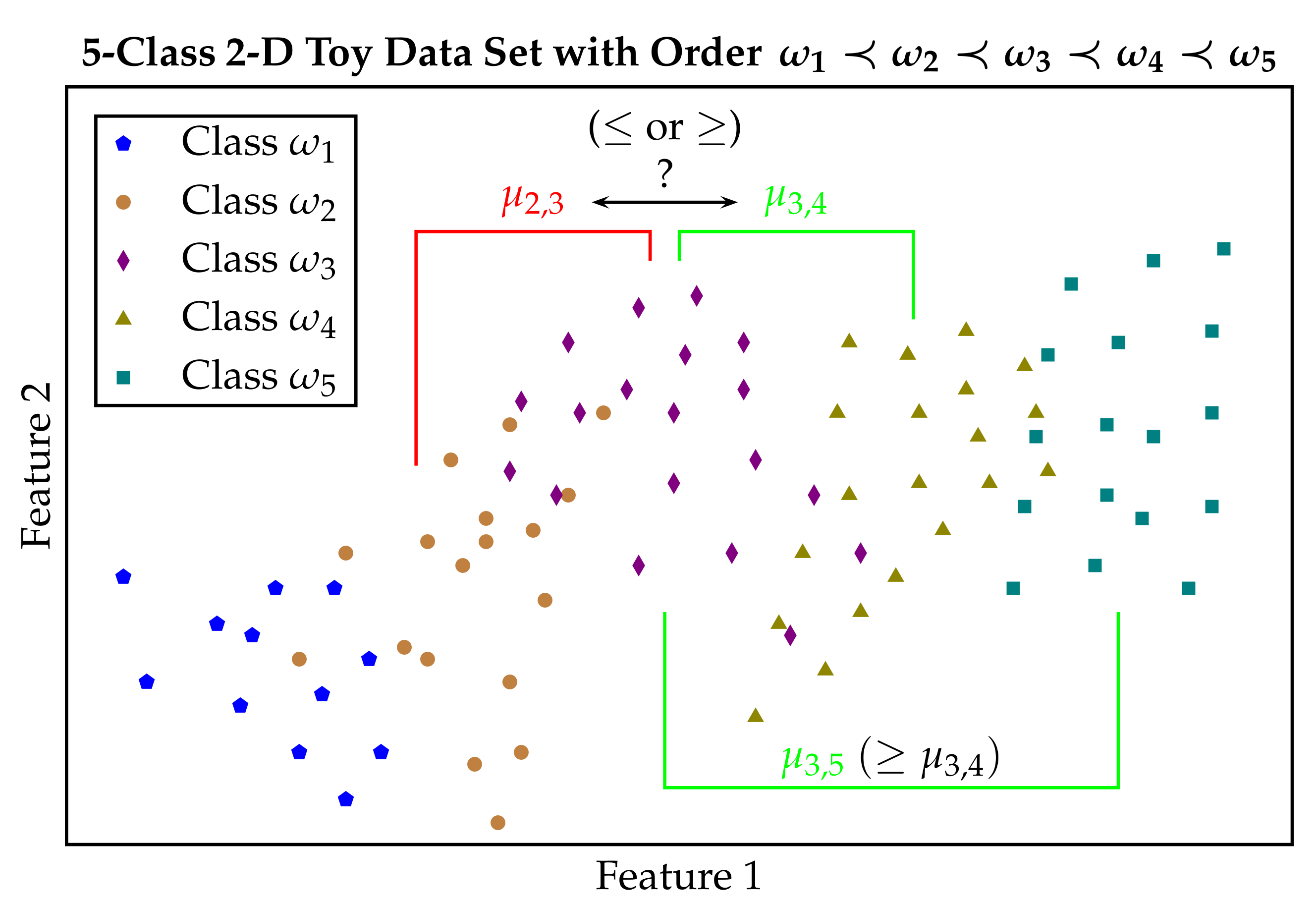
Figure 2 illustrates the properties of an ordinal classification task, based on a two-dimensional 5-class toy data set. Note that the term closer in the caption of Figure 2 does not refer to the distances between different class pairs, but to the order of the classes, i.e., the arrangement of the columns of the corresponding PSM. More precisely, e.g., for the arrangement ${\omega }_1\prec {\omega }_2\prec {\omega }_3\prec {\omega }_4\prec {\omega }_5$, we say that class ${\omega }_2$ is closer to class ${\omega }_1$ than to class ${\omega }_4$. However, for instance, the (averaged) Euclidean distance between the samples from the classes ${\omega }_2$ and ${\omega }_1$ could be greater than the (averaged) Euclidean distance between the samples from the classes ${\omega }_2$ and ${\omega }_4$.

3. Comparison to Previous Work and Additional Theoretical Outcomes

As we already implied, the current work is an extension, or even more precisely, a generalisation, of our previous study [21]. In [21], we provided a working definition for ordinal classification tasks based on the resubstitution accuracy (training accuracy) of linear support vector machines (SVMs), i.e., SVMs with linear kernels, to which we referred to as SVM-ordinal class structures. More precisely, we did not consider different options for possible LSM mappings $\mu \in {\mathcal{M}}^d$, as we propose here. Therefore, the working definition in [21] constitutes a special case of the novel approach to ordinal classification introduced in this work. However, the working definition provided in [21] led to two theoretical outcomes, i.e., a theorem for 3-class classification tasks, as well as a detection algorithm for ordinal class structures that originates from the provided definition. Moreover, with minor changes, the corresponding theorem and detection algorithm also apply to the novel generalised working definition of FS-ordinal class structures, which we briefly discuss in this section, followed by additional theoretical outcomes.

3.1. Special Case for 3-Class Classification Tasks and Detection of FS-Ordinal Structures

For the special case of $c=3$, i.e., for 3-class classification tasks, we obtain the following theorem (Theorem 1), which will be later extended as an additional theoretical outcome, at the end of this section, in Section 3.2.

Theorem 1

(FS-ordinal class structures in 3-class classification tasks). Let $X_{\Omega }\subset {\mathbb{R}}^d\times \{{\omega }_1,{\omega }_2,{\omega }_3\},d\in \mathbb{N}$, be a d-dimensional labelled data set, which constitutes a 3-class classification task. Moreover, let the corresponding PSM, M, be defined as follows, for some LSM, $\mu \in {\mathcal{M}}^d$,

$$M^{\left(id\right)}=\left(\begin{array}{ccc}0& e& f\\ e& 0& g\\ f& g& 0\end{array}\right),e,f,g>0.$$

If $e,f,g$ are pairwise distinct, i.e., $e\ne f,e\ne g$, and $f\ne g$, then there exists a permutation $\tau \in {\mathcal{T}}^3$, such that $X_{\Omega }$ constitutes an FS-ordinal classification task specific to $(\mu ,\pm \tau )$.

The proof of Theorem 1 is provided in the appendix of our previous study [21] for $e,f,g\in (0,1]$, but works analogously for $e,f,g>0$, as it is the case in the current work.

Based on our proposed working definition which is introduced in Definition 3, there exists a simple way to check for FS-ordinal class structures. A corresponding pseudo code is presented in Figure 3. Note that a numerical example for the detection algorithm depicted in Figure 3 is also provided in our previous work [21].

3.2. FS-Ordinal versus SVM-Ordinal Structures

As already mentioned above, our first approach to provide a working definition for ordinal class structures was based on pairwise resubstitution accuracies of linear SVM models. In [21], we justified the choice for such a working definition and discussed its potential, in combination with a numerical evaluation. Moreover, we also discussed the limitations of an SVM-based definition of ordinal structures. More precisely, we showed that in the case of a 3-class classification task, in which all of the possible class pairs are linearly separable, the provided detection algorithm (see Figure 3) always fails to find SVM-ordinal class structures.

However, what we did not consider in [21] is that the detection algorithm already fails if two out of the three possible class pairs of a 3-class classification task are linearly separable, as we will show shortly. This is due to the fact that the (resubstitution) accuracy is bounded to 1 (100%). As an illustrative example, let us consider a two-dimensional 3-class toy data set that is depicted in Figure 4.

From Figure 4, we can observe that the data points from class ${\omega }_1$ are linearly separable from the data points from both remaining classes ${\omega }_2$ and ${\omega }_3$, respectively. Moreover, the data points from class ${\omega }_2$ are not linearly separable from the data points from class ${\omega }_3$, in the provided two-dimensional feature space. However, the toy data set clearly constitutes an ordinal class structure with the order ${\omega }_1\prec {\omega }_2\prec {\omega }_3$, and its reversed order ${\omega }_3\prec {\omega }_2\prec {\omega }_1$. Note that for the definition of SVM-ordinal class structures, the PSM originates from the resubstitution accuracies between the corresponding class pairs. As the class pairs $({\omega }_1,{\omega }_2)$ and $({\omega }_1,{\omega }_3)$ are linearly separable, it follows that ${\mu }_{1,2}={\mu }_{1,3}=1$, and due to the symmetry (see Equation (4) for the definition of ${\mu }_{i,j}$), ${\mu }_{2,1}={\mu }_{3,1}=1$. Moreover, for the class pair $({\omega }_2,{\omega }_3)$, it clearly holds that ${\mu }_{2,3}={\mu }_{3,2}=\alpha$, with $\alpha \in (0,1)$.

Now, let us define $\tau \in {\mathcal{T}}^3$ as $\tau :(1,2,3)\mapsto (1,3,2)$, and thus $-\tau :(1,2,3)\mapsto (2,3,1)$. Then, for the PSMs, with $\mu \in {\mathcal{M}}^2$ defined as the resubstitution accuracy based on linear SVMs, we obtain the following matrices:

$$M^{\left(id\right)}=\begin{array}{c}{\omega }_1 {\omega }_2 {\omega }_3\\ \left(\begin{array}{ccc}0& 1& 1\\ 1& 0& \alpha \\ 1& \alpha & 0\end{array}\right)\end{array},\hspace{1em}{M}^{(-id)}=\begin{array}{c}{\omega }_3 {\omega }_2 {\omega }_1\\ \left(\begin{array}{ccc}0& 1& 1\\ 1& 0& \alpha \\ 1& \alpha & 0\end{array}\right)\end{array},\hspace{1em}\mathrm{and}$$

$$M^{\left(\tau \right)}=\begin{array}{c}{\omega }_1 {\omega }_3 {\omega }_2\\ \left(\begin{array}{ccc}0& 1& 1\\ 1& 0& \alpha \\ 1& \alpha & 0\end{array}\right)\end{array},\hspace{1em}{M}^{(-\tau )}=\begin{array}{c}{\omega }_2 {\omega }_3 {\omega }_1\\ \left(\begin{array}{ccc}0& 1& 1\\ 1& 0& \alpha \\ 1& \alpha & 0\end{array}\right)\end{array}.\hspace{1em}\hspace{1em}\hspace{1em}$$

Obviously, both matrices $M^{\left(id\right)}$ and $M^{\left(\tau \right)}$, and therefore their corresponding reversed counterparts, $M^{(-id)}$ and $M^{(-\tau )}$, fulfil the properties of Equation (6), and thus constitute ordinal arrangements by Definition 2. Thus, the uniqueness property of Definition 3 is violated and no (SVM-)ordinal class structure is found.

The main issue for not detecting the obvious ordinal structure of the 3-class toy data set depicted in Figure 4 is the choice of the LSM mapping $\mu$. More precisely, as we briefly discussed above, the resubstitution accuracy is bounded to the value 1. Therefore, for 3-class classification tasks, the SVM-based working definition fails in cases where at least two of the three possible class pairs are linearly separable. In this particular example, the ordinal structure would be found if the statement, ${\mu }_{1,2}<{\mu }_{1,3}$, was true. Note that, based on an eye test associated with Figure 4, the relation, ${\mu }_{1,2}<{\mu }_{1,3}$, is more intuitive than the relation ${\mu }_{1,2}={\mu }_{1,3}$. This simple example shows us why it was important to introduce the concept of LSM mappings in combination with the generalised definition of FS-ordinal class structures provided in this work.

Note that the main condition in Theorem 1 requires that the values of ${\mu }_{1,2},{\mu }_{1,3}$, and ${\mu }_{2,3}$ are pairwise distinct. The discussion of the current example showed the importance of this condition. In the current example, we had the following relations, ${\mu }_{1,2}={\mu }_{1,3}$ and ${\mu }_{2,3}<{\mu }_{1,2},{\mu }_{1,3}$. Moreover, this observation leads to a short and simple extension of Theorem 1, which we summarise in Corollary 1. Note that in contrast to the current example, in Corollary 1, we assume that the unique value (e.g., ${\mu }_{2,3}$) is greater than the two equal values (e.g., ${\mu }_{1,2}$ and ${\mu }_{1,3}$).

Corollary 1

(Extension of Theorem 1). Let $X_{\Omega }\subset {\mathbb{R}}^d\times \{{\omega }_1,{\omega }_2,{\omega }_3\},d\in \mathbb{N}$, be a d-dimensional labelled data set, which constitutes a 3-class classification task. Moreover, let the corresponding PSM, M, be defined as follows, for some LSM, $\mu \in {\mathcal{M}}^d$,

$$M^{\left(id\right)}=\left(\begin{array}{ccc}0& e& f\\ e& 0& g\\ f& g& 0\end{array}\right),e,f,g>0.$$

Furthermore, let two of the three values, $e,f,g$, be equal and smaller than the remaining one. More precisely, let one of the following three statements be true:

$$\begin{array}{cc}\hfill \left(i\right)(e=f)& \wedge (g>e=f)\hfill \\ \hfill \left(ii\right)(e=g)& \wedge (f>e=g)\hfill \\ \hfill \left(iii\right)(f=g)& \wedge (e>f=g)\hfill \end{array}$$

Then, there exists a permutation $\tau \in {\mathcal{T}}^3$, such that $X_{\Omega }$ constitutes an FS-ordinal classification task specific to $(\mu ,\pm \tau )$.

The proof of Corollary 1 is provided in the Appendix A. Note that it can be analogously shown that in the case of obtaining two equal values that are greater than the third one, e.g., $(e=f)\wedge (g<e=f)$, in combination with some LSM $\mu$, always leads to a violation of Definition 3, i.e., to the observation that the current task is not FS-ordinal specific to mapping $\mu$.

4. Classifier-Independent Level of Separability Measures

In the current section, we will first provide an example of an LSM mapping, which we will later apply in our validation experiments. Subsequently, based on the introduced LSM mapping, we will discuss a possible way of how to proceed in the case of ordinal-scaled and categorical features. Finally, we will close this section with an interpretation of the concepts provided in this work.

4.1. Discriminant Ratio

Similar to Equation (1), by $X_{\Omega }^i$, we denote the subset of $X_{\Omega }$ that consists solely of the samples from class ${\omega }_i$, i.e.,

$$X_{\Omega }^i=\{x\in X|(x,y)\in X_{\Omega }\wedge y={\omega }_i\}.$$

(9)

Moreover, by ${\overline{x}}^{\left(i\right)}$, we define the centroid of the set $X_{\Omega }^i$. More precisely, with $N_i=\left|X_{\Omega }^i\right|$ denoting the number of samples in $X_{\Omega }^i$,

$${\overline{x}}^{\left(i\right)}=\frac{1}{N_i}\sum _{x\in X_{\Omega }^i}x.$$

(10)

Furthermore, by ${\sigma }_i^2\in {\mathbb{R}}^d$, we denote the d-dimensional ($X\subset {\mathbb{R}}^d$, $d\in \mathbb{N}$) variance in $X_{\Omega }^i$, which we define as follows:

$${\sigma }_i^2=\frac{1}{N_i-1}\sum _{x\in X_{\Omega }^i}(x-{\overline{x}}^{\left(i\right)})\circ (x-{\overline{x}}^{\left(i\right)}).$$

(11)

Note that the ∘-symbol denotes the Hadamard product, also known as the Schur product, which is an element-wise product. More precisely, for $u,v\in {\mathbb{R}}^d$ with $w=u\circ v$, it holds, $w\in {\mathbb{R}}^d$ with $w_i=u_i{v}_i$, $\forall i=1,\dots ,d$.

Inspired by Fisher’s discriminant analysis [24], in this work, we define the discriminant ratio (DR) between the classes ${\omega }_i$ and ${\omega }_j$ as follows,

$$D{R}_{i,j}:=\frac{\parallel {\overline{x}}^{\left(i\right)}-{\overline{x}}^{\left(j\right)}{\parallel }^2}{\parallel {\sigma }_i^2\parallel +\parallel {\sigma }_j^2\parallel }.$$

(12)

Obviously, it holds, $D{R}_{i,j}\in {\mathbb{R}}_{\ge 0}$, and $D{R}_{i,j}$ is undefined if and only if ${\sigma }_i^2={\sigma }_j^2=0$. Therefore, $D{R}_{i,j}$ is undefined if and only if each of the sets $X_{\Omega }^i$ and $X_{\Omega }^j$ consists of solely one data point or of arbitrarily many identical data points, respectively. However, this is an unrealistic classification task scenario. Therefore, in this work, we will always assume that it holds, $\parallel {\sigma }_i^2\parallel +\parallel {\sigma }_j^2\parallel >0$.

Note that the DR measure constitutes an LSM mapping by Definition 1. More precisely, changing the class labels for the samples from class ${\omega }_i$ to ${\omega }_j$, and changing the class labels for the samples from class ${\omega }_j$ to ${\omega }_i$, obviously leads to the same $D{R}_{i,j}$ value as for the initial class labels. Therefore, the DR mapping is label invariant, and therefore fulfils property (P2) of Equation (2). Thus, we only have to check property (P1) of Equation (2), since the validity of property (P0), i.e., the non-negativity, directly follows from Equation (12).

To this end, let $Y=\{0,1\}$ be a binary label set, and $X\subset {\mathbb{R}}^d,d\in \mathbb{N}$, be a d-dimensional data set, with at least two unequal elements, i.e., $\left|X\right|>1$. For $X_Y^{*}=X\times Y$, it holds, ${\overline{x}}^{\left(0\right)}={\overline{x}}^{\left(1\right)}$, and thus $\parallel {\overline{x}}^{\left(0\right)}-{\overline{x}}^{\left(1\right)}{\parallel }^2=0$. Therefore, for $X_Y^{*}=X\times Y$, it holds that $D{R}_{0,1}=0$, which is the lower bound of the defined measure. Thus, the DR mapping fulfils property (P1) of Equation (2), and therefore constitutes an LSM mapping by Definition 1.

An exemplary illustration of the discriminant ratio-specific components is provided in Figure 5, for a 2-dimensional class pair, based on a toy data set.

4.2. Ordinal-Scaled and Categorical Features

For ordinal-scaled features, we propose to map the features to the set $\{1,\dots ,n_i\}$, whereby $n_i$ denotes the number of possible values of feature i. For instance, let us assume that feature i consists of the three feature values low < medium < high. Then, the values of feature i are transferred to the set $\{1,2,3\}$, i.e., mapping low to 1, medium to 2, and high to 3.

For categorical features, we propose to replace the mean value by the mode, i.e., the most frequent value. Let D be a d-dimensional categorical feature space. By $\Delta :D\times D\to {\{0,1\}}^d$, we denote the d-dimensional difference vector, which we define as follows. Let $x,z\in D$ be two data points from D. Furthermore, let $\delta \in {\{0,1\}}^d$ be the difference between x and z, i.e., $\delta =\Delta (x,z)$. Then, for all $i=1,\dots ,d$, the components of $\delta$ are defined as follows:

$${\delta }_i=\left\{\begin{array}{cc}0,\hfill & x_i\ne z_i,\hfill \\ 1,\hfill & x_i=z_i.\hfill \end{array}\right.$$

(13)

Note that in general, the mode is not unique. Thus, by ${\overline{M}}_i$, we denote the set of all d-dimensional mode values specific to $X_{\Omega }^i$, i.e.,

$${\overline{M}}_i=\left\{mode\left(X_{\Omega }^i\right)\right\}.$$

(14)

Therefore, for the categorical case, with $N_i=\left|X_{\Omega }^i\right|$, we define the d-dimensional variance vector, as follows:

$${\sigma }_i^{\mathrm{cat}}=\frac{1}{(N_i-1)·\left|{\overline{M}}_i\right|}\sum _{x\in X_{\Omega }^i}\sum _{{\overline{x}}_{\mathrm{cat}}\in {\overline{M}}_i}\Delta (x,{\overline{x}}_{\mathrm{cat}}).$$

(15)

Note that it is not necessary to apply the Hadamard product in the case of categorical features for the following reason: The elements of the difference vector are always equal to zero or one. Thus, squaring does not change the vector elements.

Analogously to the non-categorical case, we define the categorical discriminant ratio, denoted by DR ${}^{\mathrm{cat}}$, as follows:

$$D{R}_{i,j}^{\mathrm{cat}}:=\frac{{∥\frac{1}{|{\overline{M}}_i|+|{\overline{M}}_j|}{\sum }_{{\overline{x}}_{\mathrm{cat}}\in {\overline{M}}_i}{\sum }_{{\overline{z}}_{\mathrm{cat}}\in {\overline{M}}_j}\Delta ({\overline{x}}_{\mathrm{cat}},{\overline{z}}_{\mathrm{cat}})∥}^2}{\parallel {\sigma }_i^{\mathrm{cat}}\parallel +\parallel {\sigma }_j^{\mathrm{cat}}\parallel }.$$

(16)

As an example, we constructed a non-numerical data set that is depicted in

Table 2. Example Data Set. MSB: Medical Systems Biology. NIP: Neural Information Processing.

Author	Middle Name	Institute	ORCID	Notation
Ludwig Lausser	No	MSB	No	$x_1$
Hans A. Kestler	Yes	MSB	Yes	$x_2$
Friedhelm Schwenker	No	NIP	Yes	$x_3$

, based on the authors’ meta information.

From Table 2, we obtain the following unique 3-dimensional mode value, based on the features Middle Name, Institute, and ORCID,

$${\overline{x}}_{\mathrm{cat}}=(\mathrm{No},\mathrm{MSB},\mathrm{Yes}).$$

In combination with the obtained mode value, ${\overline{x}}_{\mathrm{cat}}$, we can compute the categorical variance as follows, based on Equation (15),

$${\sigma }^{\mathrm{cat}}=\frac{1}{3-1}\sum _{i=1}^3\Delta (x_i,{\overline{x}}_{\mathrm{cat}})=\frac{1}{2}\left[\left(\begin{array}{c}0\\ 0\\ 1\end{array}\right)+\left(\begin{array}{c}1\\ 0\\ 0\end{array}\right)+\left(\begin{array}{c}0\\ 1\\ 0\end{array}\right)\right]=\frac{1}{2}\left(\begin{array}{c}1\\ 1\\ 1\end{array}\right).$$

If we include the first author of this work to the current data set, we get the additional feature vector $x_4=(\mathrm{No},\mathrm{NIP},\mathrm{Yes})$. This leads then to two different ${\overline{x}}_{\mathrm{cat}}$ values, i.e., ${\overline{x}}_{\mathrm{cat}}\in \{(\mathrm{No},\mathrm{MSB},\mathrm{Yes}),(\mathrm{No},\mathrm{NIP},\mathrm{Yes})\}$. Note that in this example, all of the three (four) data points belong to one class, therefore we omitted the index in ${\sigma }^{\mathrm{cat}}$.

Alternatively, in the case of there being more than one mode, one could analyse whether it could be useful to randomly choose one of the corresponding mode values. This should help to reduce the computational complexity. However, this kind of evaluation is not part of the current contribution.

4.3. Interpretation

Note that one can find many mappings which fulfil the properties (P0), (P1), and (P2) of Equation (2), and thus can be identified as LSM mappings by Definition 1. For instance, it is obvious that removing the denominator from the definition of the discriminant ratio in Equation (12) also leads to an LSM mapping. More precisely, the function which solely focuses on the difference between the two centres, i.e., $\parallel {\overline{x}}^{\left(i\right)}-{\overline{x}}^{\left(j\right)}{\parallel }^2$, fulfils the properties (P0), (P1), and (P2) of Equation (2).

Therefore, in practice, it is important to choose a reasonable and task-appropriate LSM mapping. In order to remain with the current example, it is obvious that focusing on the differences between the class centres does not provide adequate—or even any—information about how easy it is to separate the corresponding classes. On the other hand, intuitively speaking, the discriminant ratio defined in Equation (12) is an appropriate measure for ranking the separability between different class pairs, in many cases.

While the motivation is clear, why it might be helpful to find ordinal structures in multi-class tasks for ordinal- and numerical-scaled features, one can argue whether it is useful to search for ordinal structures based on categorical feature spaces. To keep this discussion short, we think that, depending on the categorical features-based task at hand, it might be interesting to determine and to rank the level of separability between different class pairs, and even to find an overall class structure.

5. Evaluation

In this section, we will briefly describe a set of traditionally ordinal data sets as well as a set of traditionally non-ordinal data sets. Subsequently, we will provide the outcomes for the detection of ordinal class structures based on the resubstitution accuracy of linear SVM models and the discriminant ratio defined in Equation (12). All results were obtained using Matlab (https://www.mathworks.com/products/matlab.html, last access on 20 December 2021), applying the default parameters for the SVMs, in combination with the SMO (Sequential Minimal Optimization) solver [25,26]. At the end of the current section, we will provide a running time comparison between both LSM mappings, i.e., SVM resubstitution accuracy (SVM-Acc) and the DR measure.

Note that we apply the algorithm presented in Figure 3 for the detection of FS-ordinal structures. More precisely, a data set is identified as FS-ordinal if there exist exactly two class label permutations such that the corresponding pairwise separability matrices fulfil the properties of Equation (6). The two permutations represent the detected (bidirectional) class order.

5.1. Traditionally Ordinal Data Sets

We will evaluate the following eight, publicly available, traditionally ordinal data sets. The data sets Social Workers Decisions (SWD), Lecturers Evaluation (LEV), Employee Selection (ESL), and Employee Rejection/Acceptance (ERA) are publicly available on Weka (https://waikato.github.io/weka-wiki/datasets/, last access on 20 December 2021), and can be extracted from the file datasets_arie_ben_david.tar.gz. The data sets Contraceptive Method Choice (CMC), Car Evaluation (Cars), and Nursery are all part of the UCI machine learning repository [27]. Moreover, the BioVid Heat Pain Database (BVDB) can be obtained by request (http://www.iikt.ovgu.de/BioVid.print, last access on 20 December 2021). Note that a detailed description of the BVDB is provided in the Appendix B.

5.2. Additional Data Set Information

As one of the five classes of the Nursery data set consists of solely two data points, we will evaluate this data set as a 4-class classification task, omitting the corresponding two samples.

Due to the strong class imbalance (see

Table 3. Data Set Properties (Traditionally Ordinal Data Sets). Cl: Number of Classes. Fea: Number of Features. Sam: Number of Samples. #${\omega }_i$: Number of samples in class ${\omega }_i$.

Data Set	Cl	Fea	Sam	#${\mathit{\omega }}_1$	#${\mathit{\omega }}_2$	#${\mathit{\omega }}_3$	#${\mathit{\omega }}_4$	#${\mathit{\omega }}_5$	#${\mathit{\omega }}_6$	#${\mathit{\omega }}_7$	#${\mathit{\omega }}_8$	#${\mathit{\omega }}_9$
CMC	3	9	1473	629	511	333	−	−	−	−	−	−
LEV-4	4	4	1000	93	280	403	224	−	−	−	−	−
SWD	4	10	1000	32	352	399	217	−	−	−	−	−
Cars	4	6	1728	1210	384	69	65	−	−	−	−	−
Nursery	4	8	$\mathrm{12,958}$	4320	328	4266	4044	−	−	−	−	−
ESL-5	5	4	488	52	100	116	135	85	−	−	−	−
LEV	5	4	1000	93	280	403	197	27	−	−	−	−
BVDB	5	194	8700	1740	1740	1740	1740	1740	−	−	−	−
ERA-7	7	4	1000	92	142	181	172	158	118	137	−	−
ESL	9	4	488	2	12	38	100	116	135	62	19	4
ERA	9	4	1000	92	142	181	172	158	118	88	31	18

), often the classes 4 and 5 of the LEV data set are fused to one class. In this work, we will analyse both the initial and modified LEV data sets. We will refer to the modified 4-class data set as LEV-4.

In addition, based on the present class imbalance, in general, the classes $1,2,3$ and $7,8,9$ of the ESL data set are, respectively, combined to one class. We will evaluate both variants of the ESL data set, denoting the modified 5-class data set by ESL-5.

Similar to the data sets LEV and ESL, we will analyse two variants of the ERA data set, including the ERA-7 data set, due to the present class imbalance. We obtain the ERA-7 data set by fusing the classes $7,8,9$ to one corresponding class.

The properties of all traditionally ordinal data sets that we evaluate in this work are listed in Table 3.

5.3. Results for Traditionally Ordinal Data Sets

The evaluation of the detection of ordinal structures in combination with the traditionally ordinal data sets is provided in

Table 4. Ordinal Structure Detection (Traditionally Ordinal Data Sets). DR: Detection based on the discriminant ratio. SVM-Acc: Detection based on the linear SVM resubstitution accuracy. ✓: Ordinal class structure found. ×: No ordinal class structure found.

Type	CMC	LEV-4	SWD	Cars	Nursery	ESL-5	LEV	BVDB	ERA-7	ESL	ERA
DR	✓	✓	✓	×	×	✓	✓	✓	✓	×	✓
SVM-Acc					×				×	×	×

. From Table 4, we can make the following observations. First, based on the LSM mapping DR, eight out of the eleven data sets are identified as FS-ordinal, whereas based on the SVM-Acc measure, seven data sets are identified as FS-ordinal. Both approaches found the correct structures, i.e., the structures corresponding to the data sets’ natural class order. Second, six out of the eleven data sets are identified as FS-ordinal by both mappings simultaneously, i.e., the data sets CMC, LEV-4, SWD, ELS-5, LEV, and BVDB. Third, the data set Cars is identified as FS-ordinal in combination with the SVM-Acc measure, while not being identified as FS-ordinal based on the DR measure. On the other hand, the data sets ERA-7 and ERA are identified as FS-ordinal in combination with the DR measure, while not being identified as FS-ordinal based on the SVM-Acc measure.

The data sets Nursery and ESL were not identified as FS-ordinal by either of the two measures: DR and SVM-Acc. Obviously, FS-ordinal structures and traditionally ordinal structures constitute two different categories. Traditionally ordinal structures are defined simply based on class label names, i.e., on a semantic level. However, the corresponding order is not necessarily reflected in the feature space. As a consequence, it is not always possible to detect any structure in combination with traditionally ordinal data sets. This outcome has also been observed and discussed in [3,20,21].

5.4. Results for Traditionally Non-Ordinal Data Sets

We evaluated a set of six traditionally non-ordinal data sets that are all publicly available in the UCI machine learning repository [27]: Seeds, Forest Type Mapping (Forests), Statlog Vehicle Silhouettes (Vehicles), Statlog Image Segmentation (Segment), and Multiple Features (Mfeat). The data set properties are summarised in

Table 5. Data Set Properties (Traditionally Non-Ordinal Data Sets). Cl: Number of Classes. Fea: Number of Features. Sam: Number of Samples.

Data Set	Cl	Fea	Sam	Class Distribution
Iris	3	4	150	50 per class
Seeds	3	7	210	70 per class
Forests	4	27	523	83—86—159—195
Vehicles	4	18	846	199—212—217—218
Segment	7	19	2310	330 per class
Mfeat	10	649	2000	200 per class

.

The evaluation of the detection of ordinal structures in combination with the traditionally non-ordinal data sets is provided in

Table 6. Ordinal Structure Detection (Traditionally Non-Ordinal Data Sets). DR: Detection based on the discriminant ratio. SVM-Acc: Detection based on the linear SVM resubstitution accuracy. ✓ : Ordinal class structure found. ×: No ordinal class structure found.

Type	Iris	Seeds	Forests	Vehicles	Segment	Mfeat
DR	✓	✓	×	✓	×	×
SVM-Acc	×	✓	✓	×	×	×

. From Table 6, we can make the following observations. First, only the Seeds data set is identified as FS-ordinal simultaneously by both LSM mappings, DR and SVM-Acc, in each case specific to the class order Rosa ≺ Kama ≺ Canadian. Second, the data set Forests is identified as FS-ordinal in combination with the SVM-Acc measure, but not specific to the DR mapping. The identified class order is equal to Hinoki ≺ Sugi ≺ Mixed Deciduous ≺ Non-Forest. Third, the data sets Iris and Vehicles are identified as FS-ordinal in combination with the DR measure, while not being identified as FS-ordinal based on the SVM-Acc measure. The detected class order for the Iris data set is equal to Setosa ≺ Versicolor ≺ Virginica, whereas the detected class order for the Vehicles data set is equal to Van ≺ Bus ≺ Saab ≺ Opel.

5.5. Running Time Comparison

In

Table 7. Running Time Comparison. Cl: Number of Classes. Fea: Number of Features. Sam: Number of Samples. DR: Detection based on the discriminant ratio. SVM-Acc: Detection based on the linear SVM resubstitution accuracy. Depicted are the mean and standard deviation (std) values, for the operational time in ms, averaged over ten repetitions. For the SVM-Acc approach, for the BVDB data set, we removed the digits from the std value, for the sake of readability.

Data Set	Cl	Fea	Sam	DR	SVM-Acc
Iris	3	4	150	0.25 ± 0.14	19.97 ± 3.02
Seeds	3	7	210	0.16 ± 0.01	17.36 ± 1.61
CMC	3	9	1473	0.34 ± 0.11	1987.39 ± 2.25
Forests	4	27	523	0.42 ± 0.15	2267.25 ± 4.47
Vehicles	4	18	846	0.43 ± 0.04	9069.24 ± 13.29
LEV-4	4	4	1000	0.32 ± 0.07	70.16 ± 1.88
SWD	4	10	1000	0.34 ± 0.02	110.61 ± 1.71
Cars	4	6	1728	0.31 ± 0.02	92.20 ± 4.33
Nursery	4	8	12,958	1.76 ± 0.14	2079.20 ± 16.89
ESL-5	5	4	488	0.29 ± 0.02	52.81 ± 1.91
LEV	5	4	1000	0.40 ± 0.04	90.75 ± 2.12
BVDB	5	194	8700	44.26 ± 4.91	469,839.44 ± 2608
ERA-7	7	4	1000	1.09 ± 0.09	539.96 ± 5.43
Segment	7	19	2310	1.77 ± 0.12	13,851.62 ± 58.83
ESL	9	4	488	34.01 ± 0.43	200.59 ± 1.94
ERA	9	4	1000	77.50 ± 2.56	616.12 ± 1.61
Mfeat	10	649	2000	392.36 ± 1.13	19,661.20 ± 27.87

, we provide the averaged running time and standard deviation (std) values in ms, for both LSM mappings, DR and SVM-Acc. Note that the values are obtained by repeating the detection algorithm, which is depicted in Figure 3, for ten iterations (including the entire data set, respectively). For the experiments, we used Matlab, version R2019b, in combination with an old Intel Core i7-6700K @ 4 GHz, with the operating system Windows7, 64 bit. From Table 7, we can make the following observations.

Applying the DR measure leads to a much faster check for (FS-)ordinal structures, in comparison to applying the SVM-Acc mapping. The difference is statistically significant, according to a two-sided Wilcoxon signed-rank test [28], with a p-value of $2.93·{10}^{-4}$. The largest difference can be observed for the BVDB. Using the DR mapping leads to an averaged detection time of approximately 44 ms, whereas applying the SVM-Acc measure leads to an averaged detection time of approximately 469,839 ms, which is approximately 7.8 min, with a standard deviation of 2.6 s.

6. Discussion

In this section, we will first discuss the operational complexity of the detection of FS-ordinal class structures, based on the obtained outcomes in Section 5, including the limitations of our proposed working definition. Subsequently, we will use the simple 4-dimensional Iris data set to provide an illustrative example for the usefulness of our introduced concept of FS-ordinal class structures.

6.1. Operational Complexity and Detection Limitations

The operational cost depends on many factors, i.e., on the number of classes, the number of features, the number of samples, as well as on the choice of the corresponding LSM mapping and the complexity of the current classification task. For instance, applying the SVM-Acc measure in combination with the BVDB led to the highest averaged operational time (AOT) by far (see Table 7). The AOT for the BVDB in combination with the SVM-Acc mapping is approximately equal to 470 s, followed by the second longest AOT of approximately 20 s for the Mfeat data set. Note that the BVDB has less features than the Mfeat data set (194 to 649), and also consists of less classes (5 to 10). Obviously, the BVDB is composed of more data points than the Mfeat data set (8700 to 2000). However, on the other hand, the BVDB consists of fewer data points than the Nursery data set (8700 to 12,598), for which the AOT is only ~2 s, in combination with the SVM-Acc measure. These observations emphasise that the operational cost depends indeed on the combination of all aforementioned factors, including the complexity of the corresponding classification task.

Intuitively, the task of classifying different pain levels based on the participants’ physiological signals, such as the heart rate (BVDB), obviously seems to be more complex than differentiating between ten digits based on features such as pixel averages (Mfeat). For instance, in one of our recent studies [29], we obtained the following accuracy values. For the Mfeat data set, we obtained an averaged cross-validation (CV) accuracy of ~96%, including all 10 classes, in combination with bagging [30] and the early fusion approach [31]. In contrast, for the BVDB, including only two of the best separable classes (no pain vs. the highest pain level), we merely obtained a mean CV accuracy of about 82% (with the same size for the test folds). Implementing SVM classifiers in combination with the BVDB, very likely leads to more support vectors, in comparison to training SVM classifiers based on the Mfeat data set. An increased amount of support vectors leads to an increased amount of updating steps, and thus to a greater training duration.

As we already discussed in our previous work [21], our proposed detection algorithm reduces the detection complexity from $\mathcal{O}(c!)$ to $\mathcal{O}\left(c^2\right)$, whereby c denotes the number of classes. Note that the complexity $\mathcal{O}(c!)$ corresponds to an exhaustive search, where one has to specifically check all possible class permutations, or at least the half amount of all possible class permutations. Moreover, the sorting complexity, which is generally equal to $\mathcal{O}(c^{2}log\left(c\right))$, for the rearrangement of the rows and columns of the corresponding PSMs can be neglected. Note that, in general, the number of classes c for which we try to provide an ordinal structure analysis is usually low and mostly not (significantly) greater than 10.

As briefly discussed in Section 3.2, choosing an LSM mapping that is bounded, e.g., resubstitution accuracy which is limited to 1, i.e., 100%, can lead to failures in detecting FS-ordinal structures, even in cases where the data are linearly separably and obviously ordered, as, for instance, is depicted in Figure 4. However, one can overcome this issue by choosing an LSM mapping that can take arbitrary values, as, for instance, the DR measure, which we introduced in Equation (12). Moreover, as discussed in [32], using an accuracy-based LSM mapping might suffer from the curse of dimensionality, according to Cover’s theorem [33]. Note that we already discussed the influence of the feature dimension, based on the BVDB, for which the averaged detection time increased from roughly 44 ms specific to the DR measure, to approximately 7.8 min based on the SVM-Acc mapping. Again, one might overcome this issue by choosing an appropriate LSM mapping, such as the DR measure, which also identified the correct order of the BVDB, however in less than one second on average.

6.2. Iris Data Set—A Motivational Example for the Detection of FS-Ordinal Structures

The Iris database is one of the most frequently used traditional machine learning data sets consisting of three types of Iris flowers. The classes, i.e., Iris types, are Setosa, Versicolour, and Virginica. The data are characterised by four features, i.e., sepal length, sepal width, petal length, and petal width.

In combination with the SVM-Acc mapping, it was not able to detect an (FS-)ordinal structure specific to the Iris data set. Note that the Iris data set constitutes a 3-class classification task. This observation implies that the SVM-Acc measure-based PSM does neither fulfil the conditions of Theorem 1, nor of Corollary 1. In fact, calculating the corresponding SVM-Acc mapping-based PSM leads to

$$M^{\left(id\right)}=\begin{array}{c}{\omega }_1\hspace{1em}{\omega }_2\hspace{1em}{\omega }_3\\ \left(\begin{array}{ccc}0& 1.00& 1.00\\ 1.00& 0& 0.99\\ 1.00& 0.99& 0\end{array}\right)\end{array},$$

(17)

whereby ${\omega }_1$, ${\omega }_2$, and ${\omega }_3$ denote the classes Setosa, Versicolor, and Virginica, respectively. Note that the matrix $M^{\left(id\right)}$ from Equation (17) constitutes exactly the same example which we discussed in Section 3.2 (with $0.99=\alpha$), in combination with Figure 4. More precisely, the class orders ${\omega }_1-{\omega }_2-{\omega }_3$ (with its reversed order ${\omega }_3-{\omega }_2-{\omega }_1$) and ${\omega }_1-{\omega }_3-{\omega }_2$ (with its reversed order ${\omega }_2-{\omega }_3-{\omega }_1$) constitute ordinal arrangements by Definition 2. Therefore, the uniqueness property of Equation (8) is violated. Thus, by Definition 3, the Iris data set is not FS-ordinal with respect to the mapping SVM-Acc.

On the other hand, using the DR mapping, the Iris data set is identified as FS-ordinal specific to the order ${\omega }_1\prec {\omega }_2\prec {\omega }_3$, i.e., Setosa ≺ Versicolor ≺ Virginica (with its reversed order Virginica ≺ Versicolor ≺ Setosa). The question that arises here is the following. Does this specific structure make sense? Based solely on the label names (i.e., flower types), one would probably not try to find an ordinal structure in combination with the Iris data set. However, as we already discussed in this work, one can benefit from ordinal class structures that are present in the feature space, from a machine learning-based point of view. Note that the feature space of the Iris data set consists of solely four features (sepal length (SL), sepal width (SW), petal length (PL), and petal width (PW)), which are even easy to interpret. The low amount of features allows us to proceed with the following eye test.

From the total amount of four features, we can form six distinct binary feature combinations, i.e., (SL, SW), (SL, PL), (SL, PW), (SW, PL), (SW, PW), and (PL, PW). In Figure 6, we plotted all of the six binary feature combinations. From Figure 6, we can make the following observations. Except for the top left plot (sepal length vs. sepal width), the detected class structure (Setosa ≺ Versicolor ≺ Virginica, with its reversed order Virginica≺Versicolor ≺ Setosa) is reflected in each binary subspace. Therefore, it is to expect that the same class order is present in the complete 4-dimensional feature space. To answer the question stated above, the class order Setosa ≺ Versicolor ≺ Virginica makes sense in combination with the provided feature space. Thus, applying the proposed DR measure helped us to identify the correct class order of the Iris data set.

7. Conclusions

In this work, we provided a generalised working definition for ordinal classification (OC) tasks. To this end, we introduced the concepts of ordinal arrangements and level of separability measures (LSMs). The resulting definition of OC tasks, which is presented in Definition 3, is based on the task-specific feature space. Thus, we denote OC tasks that are identified as ordinal based on our proposed working definition, as feature space-based ordinal, i.e., FS-ordinal. Note that the definition of FS-ordinal class structures, including the corresponding concepts, is a generalisation of the recent definition approach from our previous work [21]. In the current study, we discussed one of the main limitations of our former definition and extended the corresponding theoretical outcomes. More precisely, here, we completed Theorem 1 by Corollary 1. Moreover, we presented, illustrated, and interpreted the discriminant ratio (DR), which constitutes a classifier-independent LSM mapping. Additionally, we discussed its potential for the case of categorical feature spaces, which might be an interesting research question for future studies.

We provided an exhaustive evaluation of our proposed working definition and detection algorithm, based on a set of traditionally ordinal and traditionally non-ordinal data sets, including the pain-related BioVid Heat Pain Database (BVDB). Note that the naturally occurring ordinal class structure of the BVDB, i.e., no pain $\prec \dots \prec$ unbearable pain, was correctly identified based on both our former as well as current working definition. Moreover, we were able to provide an additional motivational example for the effectiveness of our presented concepts, based on one of the oldest and most popular pattern recognition data sets, the Iris data set. Note that the Iris data set is a 4-dimensional data set consisting of three types of Iris flowers and of four easily interpretable features.

Based on the outcomes of our numerical experiments, which included a short evaluation of the corresponding detection-specific operational times, we can conclude this work as follows. We believe that we provided a non-complex working definition of ordinal class structures, i.e., FS-ordinal class structures, which benefits from the following characteristics: (i) The definition is intuitively interpretable and easy to apply; (ii) The definition focuses on the corresponding feature space; (iii) The definition allows a classifier-independent detection of (FS-)ordinal class structures; (iv) The definition can be enhanced by theoretical outcomes; and (v) The definition can be used appropriately specific to different characteristics of the corresponding classification tasks, e.g., including class imbalance or high-dimensional data.

Finally, as discussed above, the requirements of the proposed working definition do not describe a unique definition of class ordinality. This allows for a plethora of different instantiations that can imply different ordinal class structures with different characteristics. Therefore, one should be aware that not all of these class structures might be useful for specific classification tasks [34]. Thus, providing additional domain-specific definition extensions might be beneficial.